
Assessing the Influence of Different Goals in Energy Communities’ Self-Sufficiency—An Optimized Multiagent Approach


Abstract
1. Introduction
1.1. The Role of Energy Communities in the EU Agenda
1.2. Distributed Artificial Intelligence in Energy Modeling
- Purely reactive—agents decide uniquely based on the current situation, ignoring everything they have learned in the past. If-then-else or condition-action rules are usually adequate to define the actions performed by these agents.
- Model-based—agents can make decisions based on past inputs even if they cannot observe part of the environment at a given instant. Inference mechanisms using decision states and heuristics to construct decision trees are commonly used by these agents to decide which actions they will take next.
- Goal-based—agents have an explicitly represented model of the environment and deliberately choose to perform actions that they know to lead, with some probability, to the accomplishment of their goals.
- Utility-based—agents may perform actions expected to maximize their utility (function defined to measure the performance of a given choice). Multicriteria decision-making techniques can be exploited in this setting to allow agents to express preferences or define subjective probabilities, assigning coefficients of importance to the multiple criteria, etc.
- Learning—agents can improve their performance by anchoring their decisions on the knowledge gained through iterative attempts or previous experiments. Evolutionary computing or neural networks can be used if an optimal solution in a complex or large solution space is required or if an agent must decide based on patterns.
- Belief-desire-intention (BDI)—the agents’ reasoning is supported on concepts which can be used to predict human behavior: they observe the world, get and update information (beliefs), reason about their aims (desires), and, based on preferences, decide how to act to reach the objectives they are committed to (intentions).
1.3. Research Contribution and Organization
- The modeling of a LEC exploiting how goal-based residential agents (prosumagers and consumers) with different energy utilization profiles, goals and preferences influence the overall LEC operation;
- The combination of MAS and optimization methods to model and optimize the available local energy resources at the agent and the community levels;
- The evaluation of the community self-sufficiency depending on different shares of prosumager agents and the economic benefits for the agents in each scenario.
2. Methods
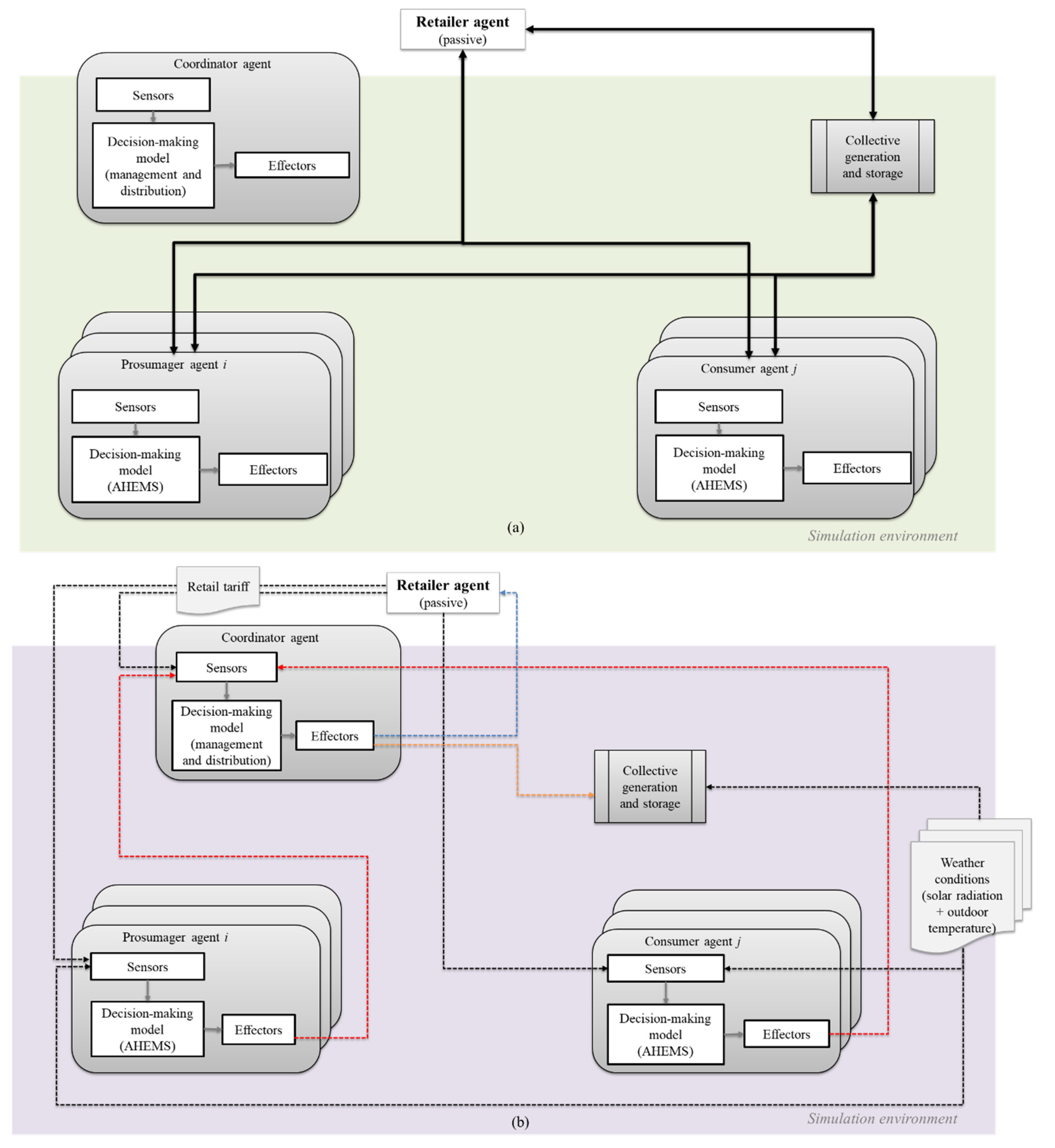
2.1. MAS Implementation
2.2. Residential Agents
2.2.1. Agents Creation and Smart Homes Modeling
- time shiftable loads, including laundry machines (LM), tumble dryers (TD) and dishwashers (DW);
- TCL, as air conditioners (AC), electric water heaters (EWH) and fridges; and
- interruptible loads, as electric vehicles (EV) and static batteries.
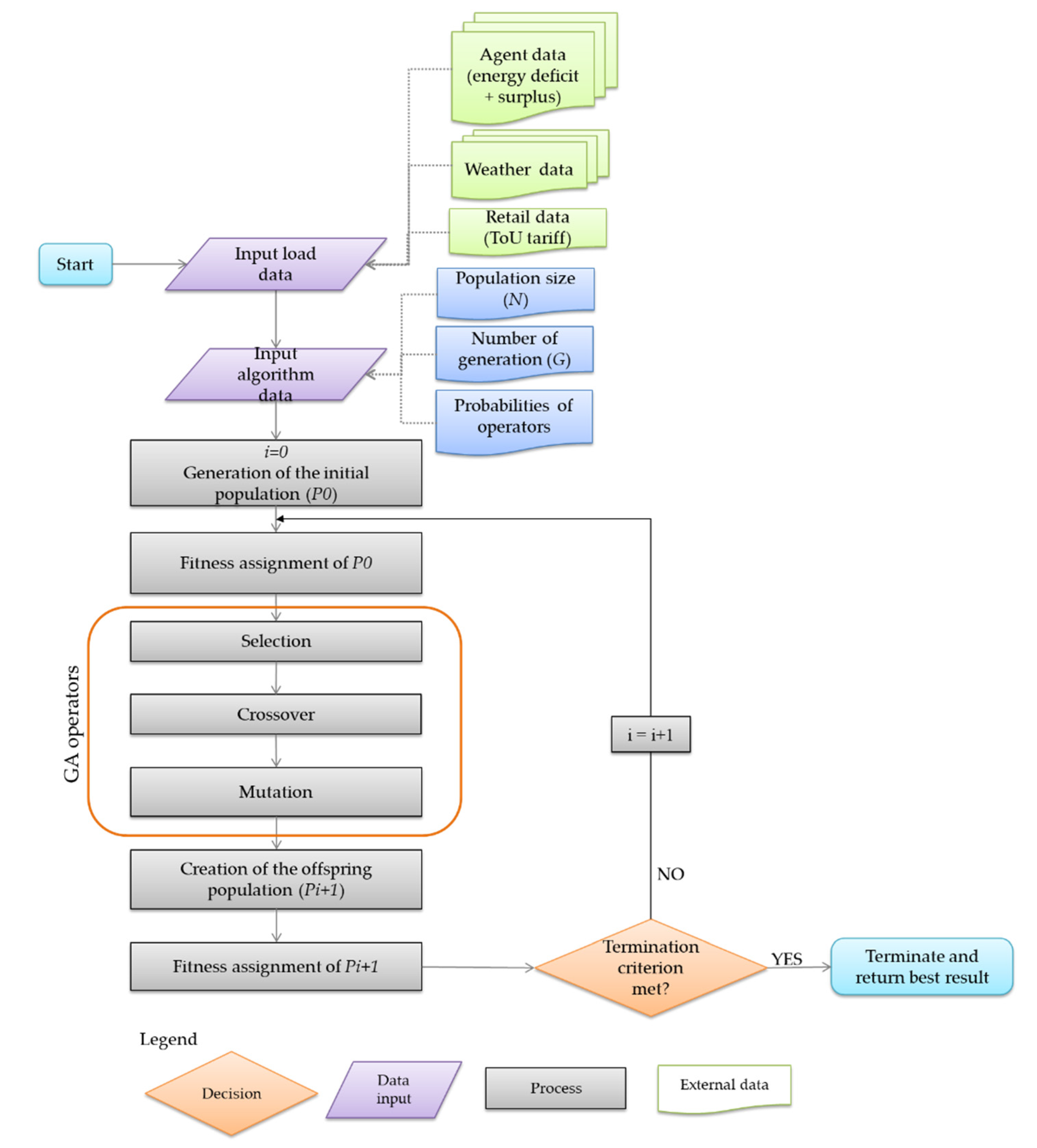
2.2.2. Optimization Framework
2.2.3. Algorithmic Approach
- swap the starting minute of the operation cycle of shiftable loads according to a given deviation bound;
- change the maximum temperature of TCL within a specified deviation limit (the minimum temperature is also influenced since the difference between maximum and minimum temperatures is assumed to be constant);
- randomly select an operation state for static and EV batteries among the four possible ones.
- swap the shiftable loads starting minute between two solutions;
- change the maximum temperatures of TCL of both parent solutions;
- change the parent solutions operation states of static and EV batteries.
2.3. Coordinator Agent
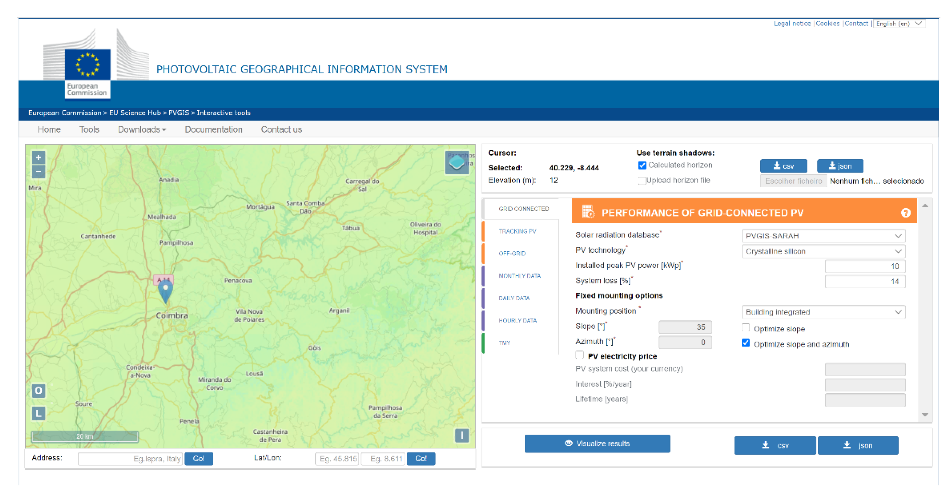
2.4. Scenario Description and Case Study
- (1)
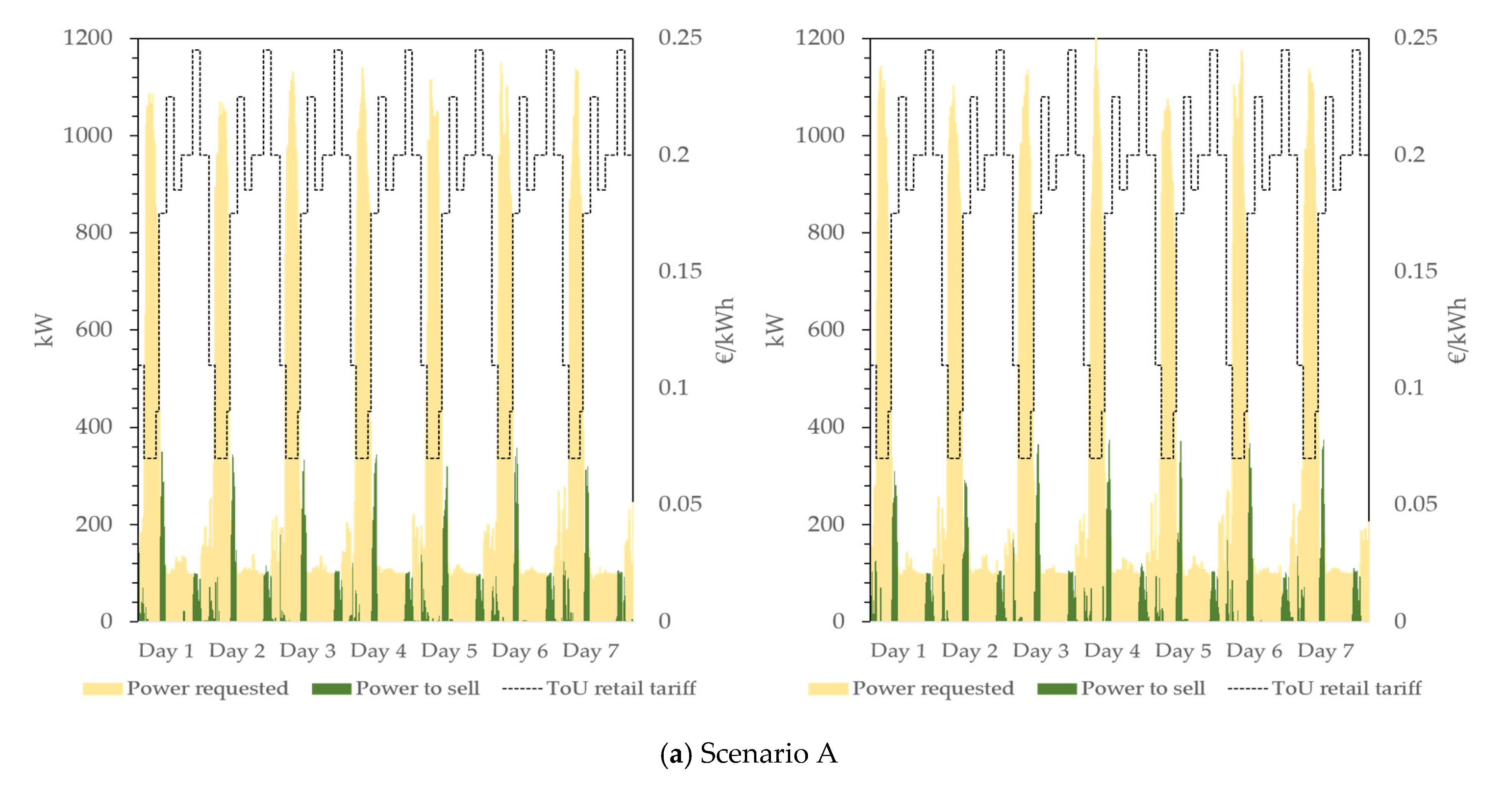
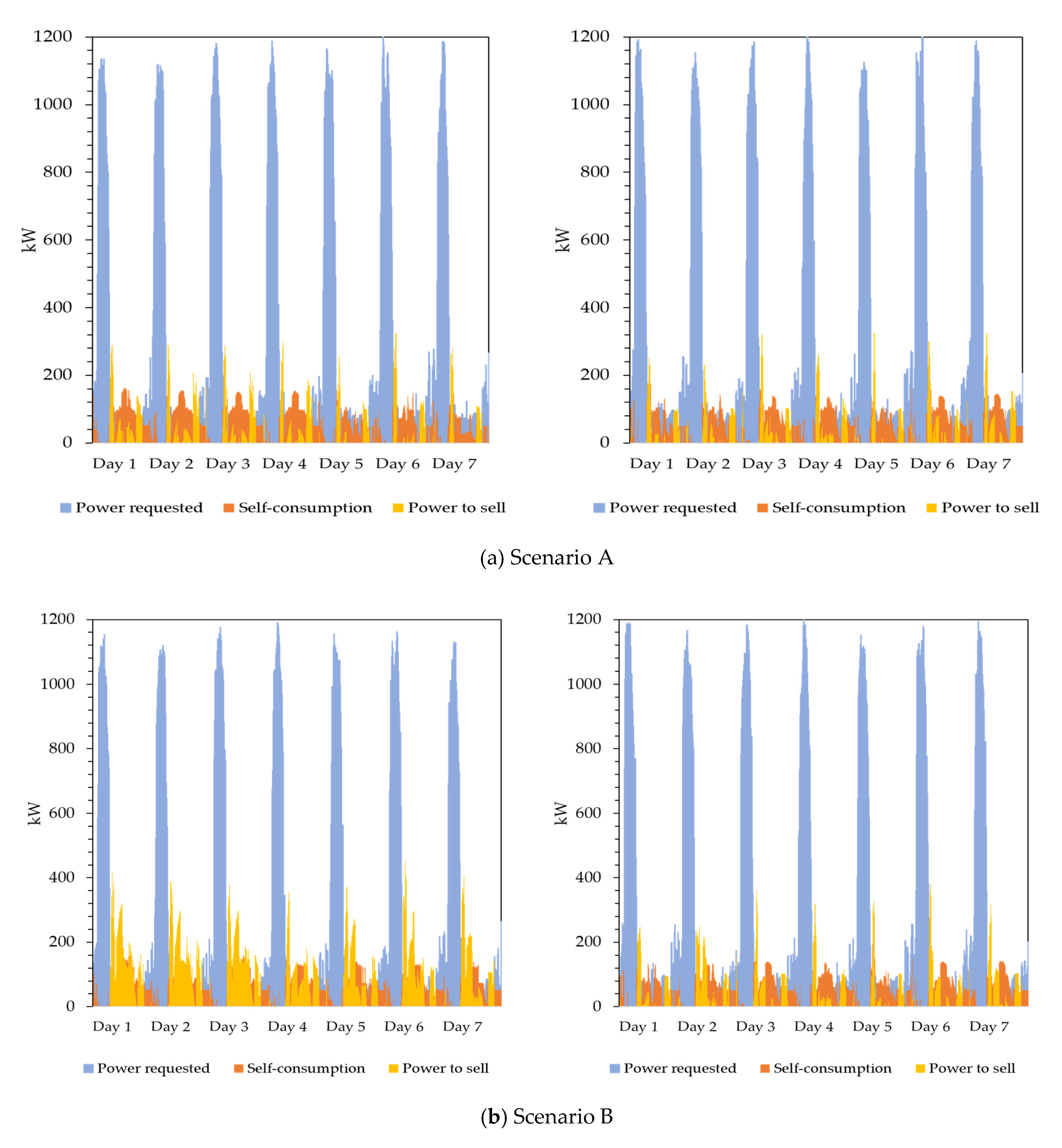
- Scenario A: consumers only;
- (2)
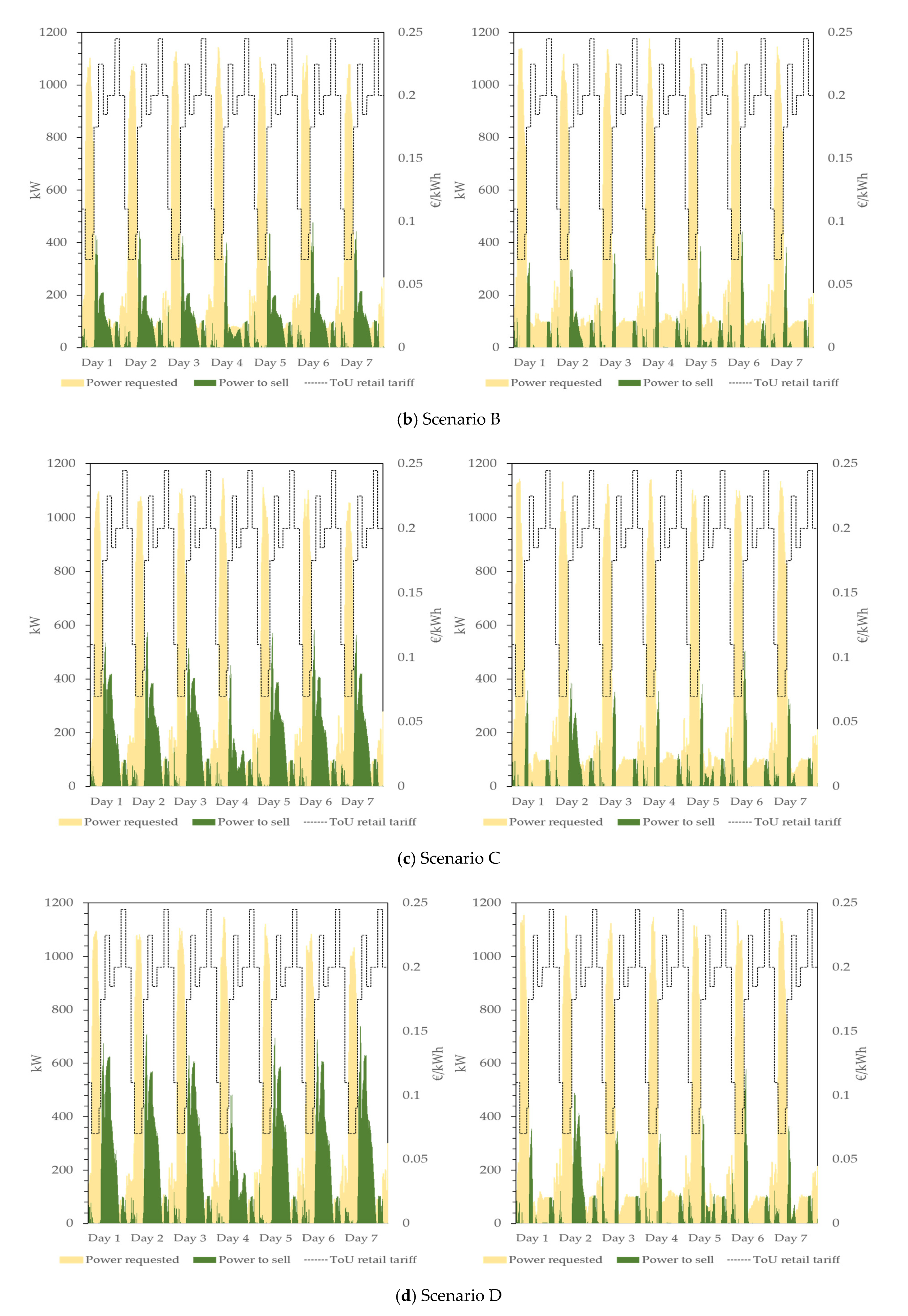
- Scenario B: 25% are prosumagers and the remaining ones are consumers;
- (3)
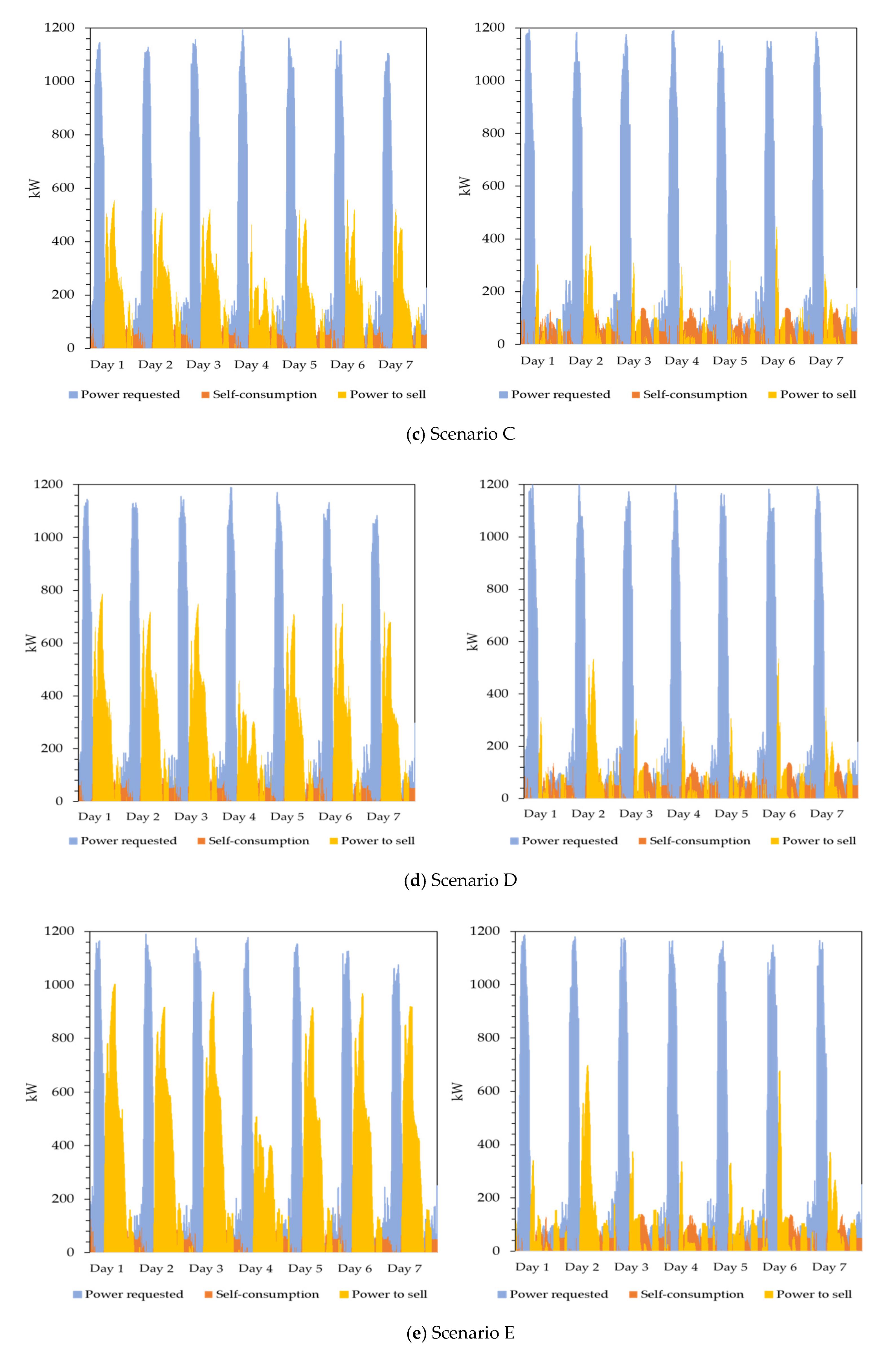
- Scenario C: 50% are prosumagers and the remaining ones are consumers;
- (4)
- Scenario D: 75% are prosumagers and the remaining ones are consumers;
- (5)
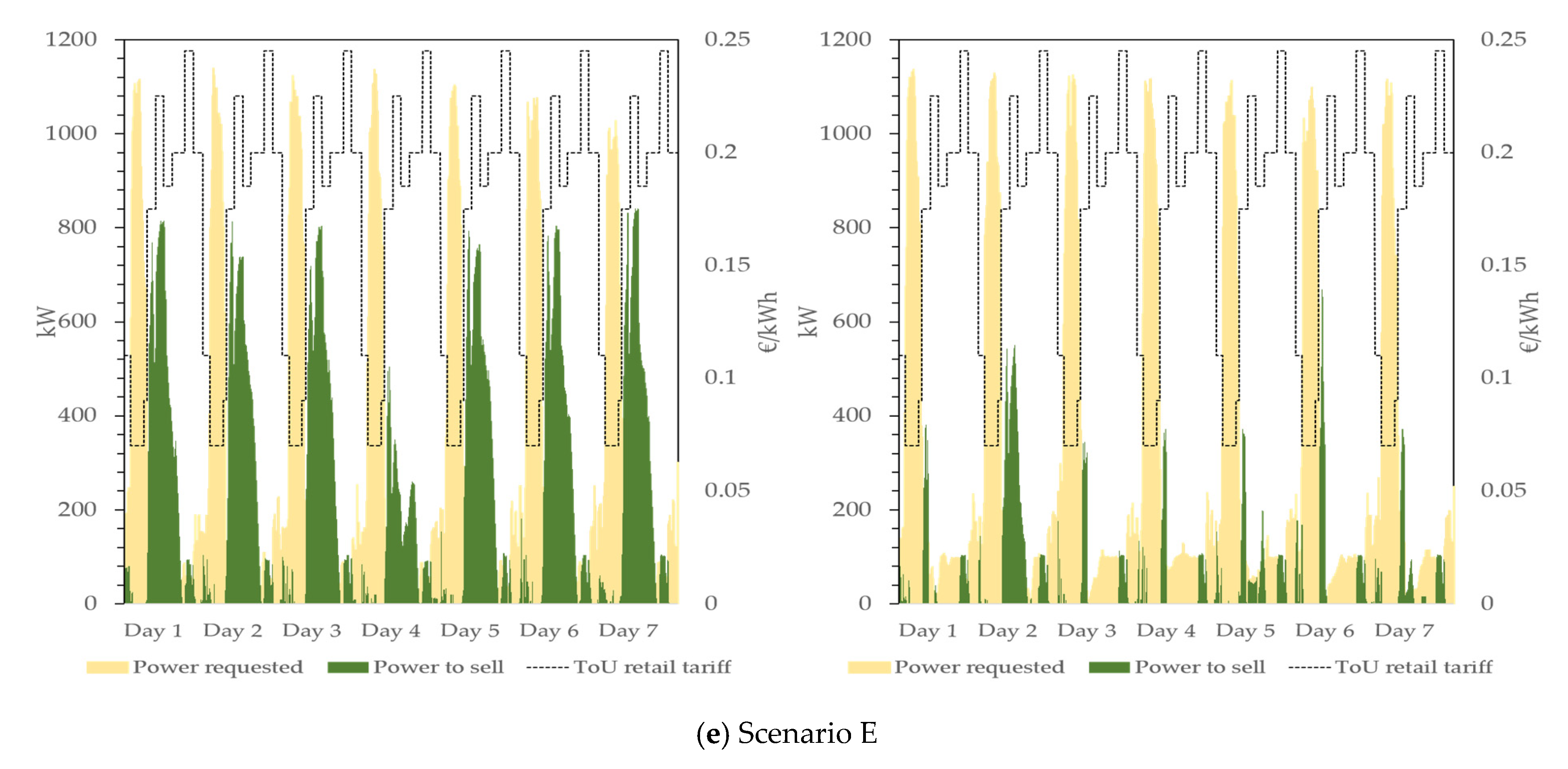
- Scenario E: prosumagers only.
3. Results and Discussion
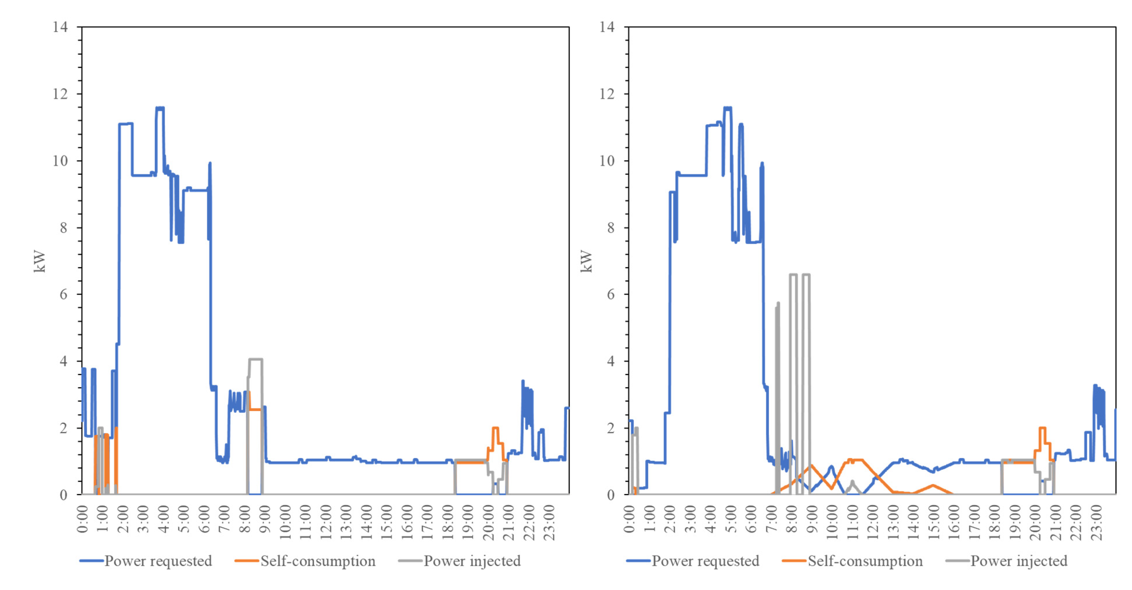
3.1. Residential agents Optimization Results
3.2. Community Operation
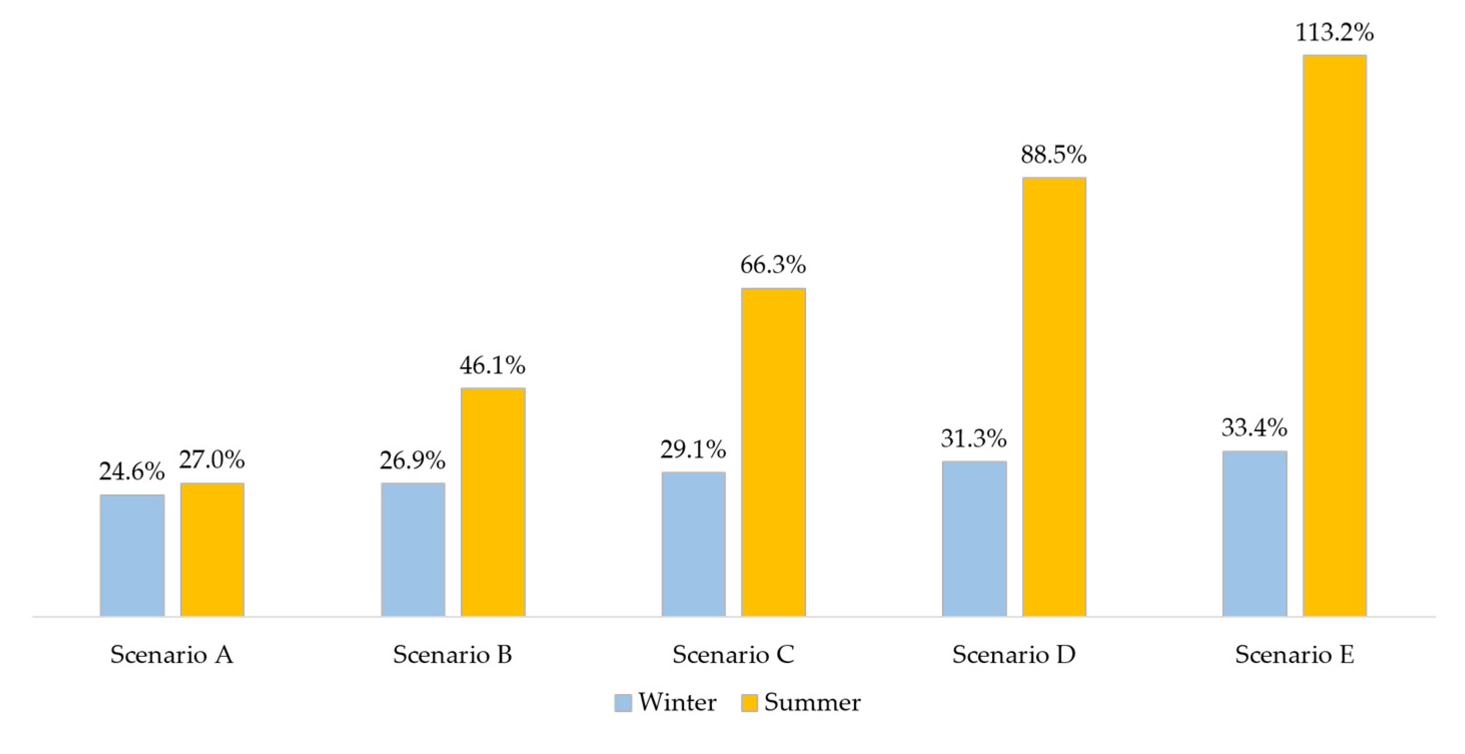
3.3. Energy Self-Sufficiency across Scenarios
3.4. Economic Benefits
4. Conclusions
Supplementary Materials
Author Contributions
Funding
Institutional Review Board Statement
Informed Consent Statement
Data Availability Statement
Conflicts of Interest
Appendix A. Residential Agents Problem Formulation

| Parameters | Decision variables | ||
|---|---|---|---|
| T | Number of time intervals the planning period is discretized into (t = 1,…, T). | Pjt | Power demanded by shiftable load j at interval t [kW]. |
| n | Number of shiftable loads (j = 1,…, n). | Pbt | Power demanded by TCL b at interval t [kW] (as defined by PBM). |
| m | Number of TCL (b = 1,…, m). | ||
| k | Number of static batteries (s = 1,…, k). | Pst | Power demanded by static battery s at interval t [kW]. |
| v | Number of EV (e = 1,…, v). | ||
| ∆t | Length of the time interval [min]. | Pet | Power demanded by EV e at interval t [kW]. |
| IFCe | Ideal final SoC for EV e [%]. | ||
| BLt | Power requested by the baseload at interval t [kW]. | PLt | Power demanded by shiftable, TCL and non-manageable baseloads at interval t [kW]. |
| BPt | Buying price at interval t [EUR/kWh]. | ||
| SPt | Selling price at interval t [EUR/kWh]. | PGrLt | Power from the grid used to supply the loads at interval t [kW]. |
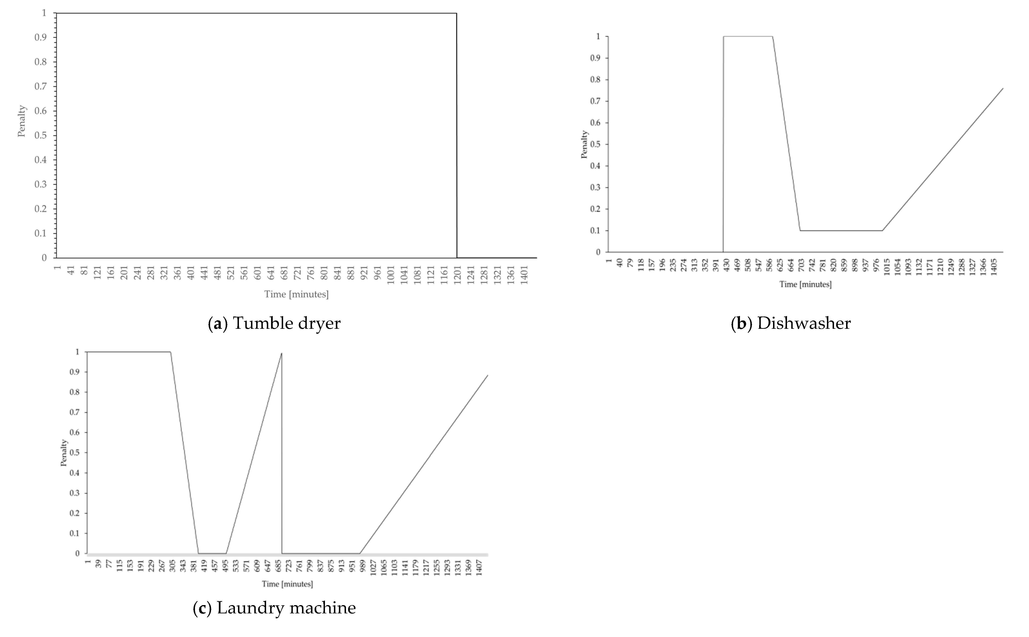
| TSPjt | Time slot penalty for shiftable load j at interval t (presented in Figure A1). | PGrEet | Power from the grid used to supply the EV battery e at interval t [kW]. |
| TVPbt | Temperature variation penalty for TCL b at interval t (as defined in Equations (10) and (11)). | PGrSst | Power from the grid used to supply the static battery s at interval t [kW]. |
| Dj | Duration of the operation cycle of shiftable load j [minutes]. | PGeLt | Power from the local generation used to supply the loads at interval t [kW]. |
| Lower temperature bound of TCL b at interval t [°C]. | PGeGrt | Local power generated injected at interval t [kW]. | |
| Upper temperature bound of TCL b at interval t [°C]. | PGeEet | Local power generated used to supply the EV battery e at interval t [kW]. | |
| Minimum SoC of static battery s [%]. | PGeSst | Local power generated used to supply the static battery s at interval t [kW]. | |
| Maximum SoC of static battery s [%]. | |||
| Minimum SoC of EV e [%]. | PELet | Power from the EV battery e used to supply the loads at interval t [kW]. | |
| Maximum SoC of EV e [%]. | |||
| fj(r) | Power requested by shiftable load j at stage r of its working cycle (r = 1,…, Dj) [kW]. | PEGret | Power injected (into the grid or the community) by the EV battery e at interval t [kW]. |
| PGt | Expected local generation at interval t [kW]. | PSLt | Power from the static battery s used to supply the loads at interval t [kW]. |
| θbt | Temperature of the space being heated/cooled by the TCL b at interval t (as defined in Equation (1)) [°C]. | PSGrst PSt | Power injected (into the grid or the community) by the static battery s at interval t [kW]. Total power injected at interval t [kW]. |
| ηech/ηedch | Charging/discharging efficiency of the battery of EV e [-]. | SCt Yjt | Total power used for self-consumption at interval t [kW]. Binary variable representing whether shiftable load j is operating at interval t. |
| ηsch/ηsdch | Charging/discharging efficiency of the static battery s [-]. | ||
| Cape | Capacity of the battery of EV e [kW]. | Starting interval of the working cycle of shiftable load j. | |
| Caps | Capacity of static battery s [kW]. | ||
| SOCst | SoC of static battery s at interval t [%]. | ||
| SOCet | SoC of EV e at interval t [%]. | ||
Appendix B. Time Slot Penalties of Shiftable Loads

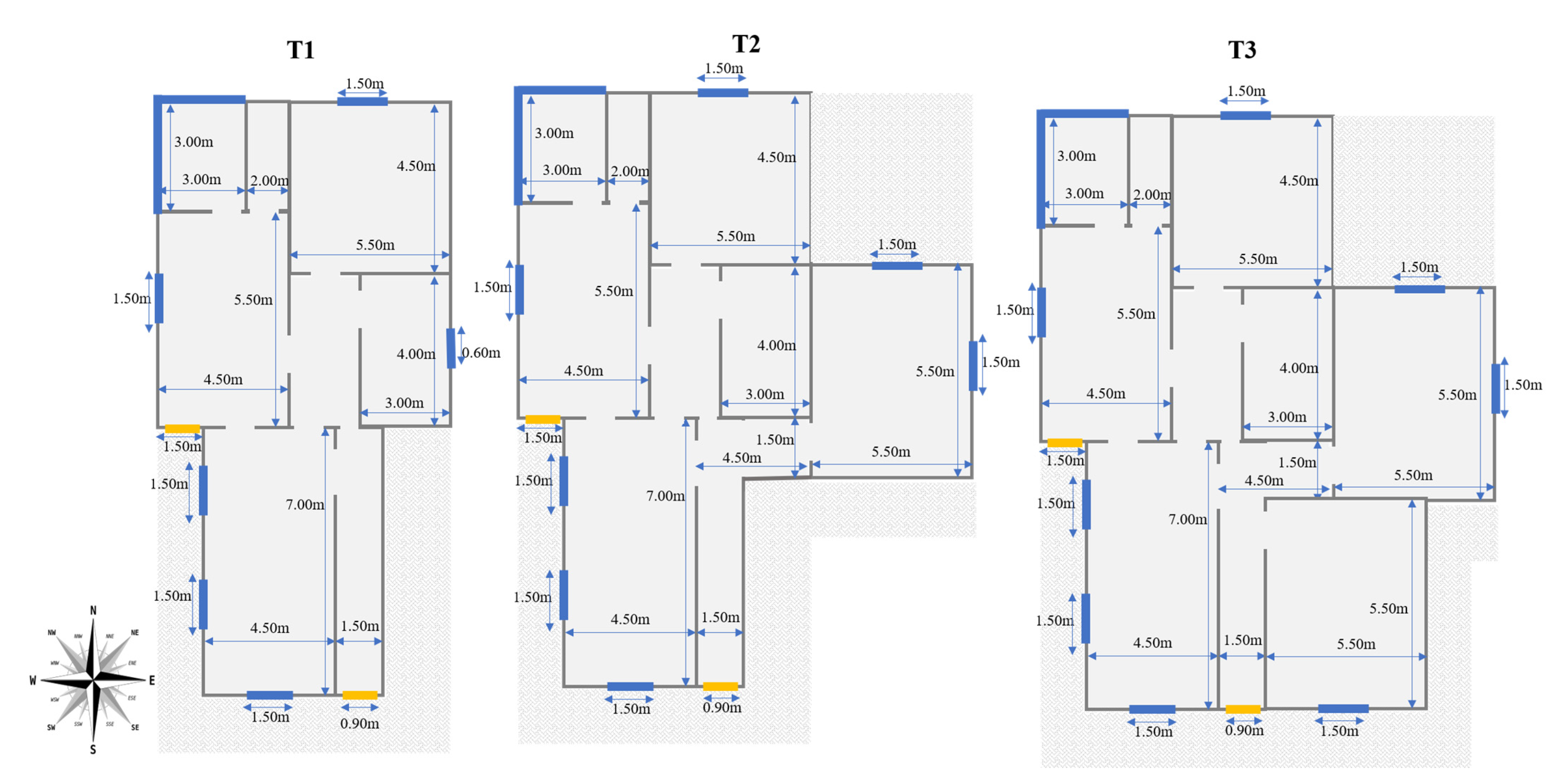
Appendix C. Dwellings Characteristics

Appendix D. Overall Community Performance


References
- Rae, C.; Bradley, F. Energy autonomy in sustainable communities—A review of key issues. Renew. Sustain. Energy Rev. 2012, 16, 6497–6506. [Google Scholar] [CrossRef]
- Gui, E.M.; MacGill, I. Typology of future clean energy communities: An exploratory structure, opportunities, and challenges. Energy Res. Soc. Sci. 2018, 35, 94–107. [Google Scholar] [CrossRef]
- Koirala, B.P.; Araghi, Y.; Kroesen, M.; Ghorbani, A.; Hakvoort, R.A.; Herder, P.M. Trust, awareness, and independence: Insights from a socio-psychological factor analysis of citizen knowledge and participation in community energy systems. Energy Res. Soc. Sci. 2018, 38, 33–40. [Google Scholar]
- Klaimi, J.; Rahim-Amoud, R.; Merghem-Boulahia, L. Energy management in the smart grids via intelligent storage systems. In Agent-Based Modeling of Sustainable Behaviors; Alonso-Betanzos, A., Sánchez-Maroño, N., Fontenla-Romero, O., Polhill, J.G., Craig, T., Bajo, J., Corchado, J.M., Eds.; Springer International Publishing AG: Cham, Switzerland, 2017; pp. 227–250. [Google Scholar]
- European Committee of the Regions. Models of Local Energy Ownership and the Role of Local Energy Communities in Energy Transition in Europe. 2018. Available online: https://op.europa.eu/en/publication-detail/-/publication/667d5014-c2ce-11e8-9424-01aa75ed71a1/language-en (accessed on 7 June 2020).
- REScoop.EU. The New Energy Market Design: How the EU Can Support Energy Communities and Citizens to Participate in the Energy Transition. 2018. Available online: https://energy-cities.eu/wp-content/uploads/2018/11/commuity_energy_coalition_pp_trilogues_mdi_final.pdf (accessed on 7 June 2020).
- Caramizaru, A.; Uihlein, A. Energy Communities: An Overview of Energy and Social Innovation. Belgium, 2020. Available online: https://ec.europa.eu/jrc/en/publication/eur-scientific-and-technical-research-reports/energy-communities-overview-energy-and-social-innovation (accessed on 2 November 2020).
- Braunholtz-Speight, T.; Sharmina, M.; Manderson, E.; McLachlan, C.; Hannon, M.; Hardy, J.; Mander, S. Evolution of Community Energy in the UK. 2018. Available online: https://d2e1qxpsswcpgz.cloudfront.net/uploads/2020/03/ukerc-wp_evolution-of-community-energy-in-the-uk.pdf (accessed on 16 August 2020).
- Hahnel, U.J.J.; Herberz, M.; Pena-Bello, A.; Parra, D.; Brosch, T. Becoming prosumer: Revealing trading preferences and decision-making strategies in peer-to-peer energy communities. Energy Policy 2019, 137, 111098. [Google Scholar] [CrossRef]
- European Commission. Directive on the Promotion of the Use of Energy from Renewable Sources (Recast); European Commission: Brussels, Belgium, 2018; Available online: https://eur-lex.europa.eu/legal-content/en/TXT/?uri=CELEX%3A32018L2001 (accessed on 15 June 2020).
- European Parliament and Council of the EU. Directive on Common Rules for the Internal Market for Electricity. 2019. Available online: https://eur-lex.europa.eu/legal-content/EN/TXT/?uri=CELEX%3A32019L0944 (accessed on 15 June 2020).
- Lowitzsch, J.; Hoicka, C.E.; van Tulder, F.J. Renewable energy communities under the 2019 European Clean Energy Package—Governance model for the energy clusters of the future? Renew. Sustain. Energy Rev. 2020, 122, 109489. [Google Scholar] [CrossRef]
- Sloot, D.; Jans, L.; Steg, L. Is it for the money, the environment, or the community? Motives for being involved in community energy initiatives. Glob. Environ. Chang. 2019, 57, 101936. [Google Scholar] [CrossRef]
- Engelken, M.; Römer, B.; Drescher, M.; Welpe, I. Transforming the energy system: Why municipalities strive for energy self-sufficiency. Energy Policy 2016, 98, 365–377. [Google Scholar]
- Dóci, G.; Vasileiadou, E. “Let’s do it ourselves”—Individual motivations for investing in renewables at community level. Renew. Sustain. Energy Rev. 2015, 49, 41–50. [Google Scholar]
- Ruppert-Winkel, C.; Hauber, J. Changing the energy system towards renewable energy self-sufficiency—A multi-perspective and interdisciplinary framework. Sustainability 2014, 6, 2822–2831. [Google Scholar]
- Müller, M.O.; Stämpfli, A.; Dold, U.; Hammer, T. Energy autarky: A conceptual framework for sustainable regional development. Energy Policy 2011, 39, 5800–5810. [Google Scholar]
- Pieńkowski, D.; Zbaraszewski, W. Sustainable energy autarky and the evolution of German bioenergy villages. Sustainability 2019, 11, 4996. [Google Scholar] [CrossRef]
- Bentley, E.; Kotter, R.; Wang, Y.; Das, R.; Putrus, G.; Van Der Hoogt, J.; Van Bergen, E.; Warmerdam, J.; Heller, R.; Jablonska, B. Pathways to energy autonomy–Challenges and opportunities. Int. J. Environ. Stud. 2019, 76, 893–921. [Google Scholar] [CrossRef]
- Campos, G.I.; Esther, M.G.; Swantje, G.; Stephen, H.; Lars, H. Regulatory challenges and opportunities for collective renewable energy prosumers in the EU. Energy Policy 2020, 138, 111212. [Google Scholar]
- McKenna, E.; Leicester, P.; Webborn, E.; Elam, S. Analysis of international residential solar PV self-consumption. In ECEEE Summer Study Proceedings; ECEEE: Stockholm, Sweden, 2019; pp. 707–716. [Google Scholar]
- Strbac, G. Demand-side management: Benefits and challenges. Energy Policy 2008, 36, 4419–4426. [Google Scholar] [CrossRef]
- Gelazanskas, L.; Gamage, K.A.A. Demand side management in smart grid: A review and proposals for future direction. Sustain. Cities Soc. 2014, 11, 22–30. [Google Scholar] [CrossRef]
- Schill, W.-P.; Zerrah, A.; Kunz, F. Prosumage of Solar Electricity: Pros, Cons, and the System Perspective. 2017. DIW Berlin Discussion Paper No. 1637. Available online: https://ssrn.com/abstract=2912814 (accessed on 19 July 2019).
- Kiaee, M.; Cruden, A. Estimation of cost savings from participation of electric vehicles in vehicle to grid (V2G) schemes. J. Mod. Power Syst. Clean Energy 2015, 3, 249–258. [Google Scholar] [CrossRef]
- Antonopoulos, I.; Robu, V.; Couraud, B.; Kirli, D.; Norbu, S.; Kiprakis, A.; Wattam, S. Artificial intelligence and machine learning approaches to energy demand-side response: A systematic review. Renew. Sustain. Energy Rev. 2020, 130, 109899. [Google Scholar] [CrossRef]
- Ma, T.; Nakamori, Y. Modeling technological change in energy systems—From optimization to agent-based modeling. Energy 2009, 34, 873–879. [Google Scholar] [CrossRef]
- Ali, S.S.; Choi, B.J. State-of-the-art of artificial intelligence techniques for distributed smart grids: A review. Electronics 2020, 9, 1030. [Google Scholar] [CrossRef]
- Chaib-Draa, B.; Moulin, B.; Mandiau, R.; Millot, P. Trends in Distributed Artificial Intelligence. Artif. Intell. Rev. 1992, 6, 35–66. [Google Scholar] [CrossRef]
- Merabet, H.G.; Essaaidi, M.; Talei, H.; Abid, R.M.; Khalil, N.; Madkour, M.; Benhaddou, D. Applications of multi-agent systems in smart grids: A survey. In Proceedings of the International Conference on Multimedia Computing and Systems, Marrakech, Morocco, 14–16 April 2014; pp. 1088–1094. [Google Scholar]
- Chmieliauskas, A.; Davis, C.B.; Bollinger, L.A. Next steps in modelling socio-technical systems: Towards collaborative modelling. In Agent-Based Modelling of Socio-Technical Systems; Van Dam, K., Nikolic, I., Lukszo, Z., Eds.; Springer: Dordrecht, The Netherlands, 2013; Volume 9. [Google Scholar]
- Coelho, V.N.; Cohen, M.W.; Coelho, I.M.; Liu, N.; Guimarães, F.G. Multi-agent systems applied for energy systems integration: State-of-the-art applications and trends in microgrids. Appl. Energy 2017, 187, 820–832. [Google Scholar] [CrossRef]
- Lez-Briones, A.G.; de la Prieta, F.; Mohamad, M.S.; Omatu, S.; Corchado, J.M. Multi-agent systems applications in energy optimization problems: A state-of-the-art review. Energies 2018, 11, 1928. [Google Scholar] [CrossRef]
- Allab, M.M.I.T.; Ne, M.I.T.M.; Square, T. The Agent Network Architecture (ANA). ACM SIGART Bull. 1991, 2, 115–120. [Google Scholar]
- Chin, K.O.; Anthony, P.; Lukose, D. Agent architecture: An overview. Trans. Sci. Technol. 2014, 1, 18–35. [Google Scholar]
- Dijkema, G.P.J.; Lukszo, Z.; Weijnen, M.P.C. Introduction. In Agent-Based Modelling of Socio-Technical Systems; Van Dam, K., Nikolic, I., Lukszo, Z., Eds.; Springer: Dordrecht, The Netherlands, 2013; Volume 9. [Google Scholar]
- Guo, Y.; Zeman, A.; Li, R. Utility simulation tool for automated energy demand side management. In First International Workshop on Agent Technology for Energy Systems (ATES 2010); International Foundation for Autonomous Agents and Multiagent Systems: Toronto, Canada, 2010; pp. 37–44. [Google Scholar]
- Ringler, P.; Keles, D.; Fichtner, W. Agent-based modelling and simulation of smart electricity grids and markets—A literature review. Renew. Sustain. Energy Rev. 2016, 57, 205–215. [Google Scholar] [CrossRef]
- Bunn, D.W.; Oliveira, F.S. Agent-based analysis of technological diversification and specialization in electricity markets. Eur. J. Oper. Res. 2007, 181, 1265–1278. [Google Scholar] [CrossRef]
- Radhakrishnan, B.M.; Srinivasan, D. A multi-agent based distributed energy management scheme for smart grid applications. Energy 2016, 103, 192–204. [Google Scholar] [CrossRef]
- Davarzani, S.; Granell, R.; Taylor, G.A.; Pisica, I. Implementation of a novel multi-agent system for demand response management in low-voltage distribution networks. Appl. Energy 2019, 253, 113516. [Google Scholar] [CrossRef]
- Rai, V.; Henry, A.D. Agent-based modelling of consumer energy choices. Nat. Clim. Chang. 2016, 6, 556–562. [Google Scholar] [CrossRef]
- Evora, J.; Kremers, E.; Morales, S.; Hernandez, M.; Hernandez, J.J.; Viejo, P. Agent-based modelling of electrical load at household level. In Cosmos 2011—Proceedings of the 2011 Workshop on Complex Systems Modelling and Simulation; Luniver Press: Beckington, UK, 2011; pp. 1–15. [Google Scholar]
- Lin, H.; Wang, Q.; Wang, Y.; Liu, Y.; Sun, Q.; Wennersten, R. The energy-saving potential of an office under different pricing mechanisms—Application of an agent-based model. Appl. Energy 2017, 202, 248–258. [Google Scholar] [CrossRef]
- Kahrobaee, S.; Rajabzadeh, R.A.; Soh, L.K.; Asgarpoor, S. Multiagent study of smart grid customers with neighborhood electricity trading. Electr. Power Syst. Res. 2014, 111, 123–132. [Google Scholar] [CrossRef]
- Morsali, R.; Thirunavukkarasu, G.S.; Seyedmahmoudian, M.; Stojcevski, A.; Kowalczyk, R. A relaxed constrained decentralised demand side management system of a community-based residential microgrid with realistic appliance models. Appl. Energy 2020, 277, 115626. [Google Scholar] [CrossRef]
- Zhao, Z.; Lee, W.C.; Shin, Y.; Song, K.B. An optimal power scheduling method for demand response in home energy management system. IEEE Trans. Smart Grid 2013, 4, 1391–1400. [Google Scholar] [CrossRef]
- Salinas, S.; Li, M.; Li, P. Multi-objective Optimal Energy Consumption Scheduling in Smart Grids. IEEE Trans. Smart Grid 2013, 4, 341–348. [Google Scholar] [CrossRef]
- Logenthiran, T.; Srinivasan, D.; Shun, T.Z. Demand side management in smart grid using heuristic optimization. IEEE Trans. Smart Grid 2012, 3, 1244–1252. [Google Scholar] [CrossRef]
- Frangopoulos, C.A. Optimization methods for energy systems. In Exergy, Energy System Analysis and Optimization; Encyclopedia of Life Support Systems (EOLSS): Paris, France, 2017; Volume 2, pp. 233–258. [Google Scholar]
- Zafar, R.; Mahmood, A.; Razzaq, S.; Ali, W.; Naeem, U.; Shehzad, K. Prosumer based energy management and sharing in smart grid. Renew. Sustain. Energy Rev. 2018, 82, 1675–1684. [Google Scholar] [CrossRef]
- Vinyals, M.; Velay, M.; Sisinni, M. A multi-agent system for energy trading between prosumers. In Distributed Computing and Artificial Intelligence, Proceedings of the 14th International Symposium on Distributed Computing and Artificial Intelligence, Porto, Portugal, 21–23 June 2017; Springer: Cham, Switzerland, 2017; Volume 620, pp. 215–222. [Google Scholar]
- Xiong, L.; Li, P.; Wang, Z.; Wang, J. Multi-agent based multi objective renewable energy management for diversified community power consumers. Appl. Energy 2020, 259, 114140. [Google Scholar] [CrossRef]
- Portuguese Statistics Institute. Households in 2011 Census: How Portuguese Households Have Evolved? pp. 1–26, 2013. Available online: https://www.ine.pt/ngt_server/attachfileu.jsp?look_parentBoui=207999200&att_display=n&att_download=y (accessed on 4 April 2019).
- Dusparic, I.; Taylor, A.; Marinescu, A.; Golpayegani, F.; Clarke, S. Residential demand response: Experimental evaluation and comparison of self-organizing techniques. Renew. Sustain. Energy Rev. 2017, 80, 1528–1536. [Google Scholar] [CrossRef]
- Gomes, Á.; Antunes, C.H.; Martinho, J. A physically-based model for simulating inverter type air conditioners/heat pumps. Energy 2013, 50, 110–119. [Google Scholar] [CrossRef]
- Soares, A.; Antunes, C.H.; Oliveira, C. A customized evolutionary algorithm for multiobjective management of residential energy resources. IEEE Trans. Ind. Inform. 2017, 13, 492–501. [Google Scholar] [CrossRef]
- Gonçalves, I.; Gomes, Á.; Antunes, C.H. Optimizing the management of smart home energy resources under different power cost scenarios. Appl. Energy 2019, 242, 351–363. [Google Scholar] [CrossRef]
- Laguerre, O.; Flick, D. Temperature prediction in domestic refrigerators: Deterministic and stochastic approaches. Int. J. Refrig. 2010, 33, 41–51. [Google Scholar] [CrossRef]
- Hovgaard, T.G.; Larsen, L.F.S.; Edlund, K.; Jørgensen, J.B. Model predictive control technologies for efficient and flexible power consumption in refrigeration systems. Energy 2012, 44, 105–116. [Google Scholar] [CrossRef]
- Lopes, M.; Antunes, C.H.; Reis, I.; Martins, A.G. A multidisciplinary approach to assess end-users’ preferences and quantify electricity demand flexibility. In Proceedings of the BEHAVE 2018—5th European Conference on Behaviour and Energy Efficiency, Zurich, Switzerland, 5–7 September 2018; pp. 229–230. [Google Scholar]
- Rasouli, V.; Goncalves, I.; Antunes, C.H.; Gomes, A. A Comparison of MILP and metaheuristic approaches for implementation of a home energy management system under dynamic tariffs. In Proceedings of the 2nd International Conference on Smart Energy Systems and Technologies (SEST), Porto, Portugal, 9–11 September 2019. [Google Scholar]
- Reeves, C.R. Genetic Algorithms. In Handbook of Metaheuristics, 3rd ed.; Gendreau, M., Potvin, J.Y., Eds.; Springer: Berlin/Heidelberg, Germany, 2019; Volume 146, pp. 109–139. [Google Scholar]
- Gonçalves, I.; Gomes, Á.; Antunes, C.H. Optimizing residential energy resources with an improved multi-objective genetic algorithm based on greedy mutations. In Proceedings of the Genetic and Evolutionary Computation Conference (GECCO), Kyoto, Japan, 15–19 July 2018; Association for Computing Machinery: New York, NY, USA, 2018; pp. 1246–1253. [Google Scholar]
- Deb, K.; Pratap, A.; Agarwal, S.; Meyarivan, T. A fast and elitist multiobjective genetic algorithm: NSGA-II. IEEE Trans. Evol. Comput. 2002, 6, 182–197. [Google Scholar] [CrossRef]
- Reis, I.F.G.; Gonçalves, I.; Lopes, M.A.R.; Antunes, C.H. A multi-agent system approach to exploit demand-side flexibility in an energy community. Util. Policy 2020, 67, 101114. [Google Scholar] [CrossRef]
- Brady, J.; O’Mahony, M. Modelling charging profiles of electric vehicles based on real-world electric vehicle charging data. Sustain. Cities Soc. 2016, 26, 203–216. [Google Scholar] [CrossRef]
- Portuguese Energy Regulator. Tariffs and prices—Electricity. Tariffs and Prices for Electricity and Other Services in 2020. Available online: https://www.erse.pt/media/xcwb23n2/tarifaspreços2020.pdf (accessed on 22 January 2020).
- IEA. Residential Prosumers—Drivers and Policy Options (Re-Prosumers). 2014. Available online: http://iea-retd.org/wp-content/uploads/2014/06/RE-PROSUMERS_IEA-RETD_2014.pdf (accessed on 3 April 2019).
- Portuguese Government. Law 40/90. Lisbon. 1990. Available online: https://dre.pt/application/conteudo/334611 (accessed on 17 February 2020).
- Portuguese Government Ordinance 379-A/2013. Available online: https://dre.pt/application/conteudo/70789581 (accessed on 17 February 2020).
- The European Commission. EU Building Database. 2018. Available online: https://ec.europa.eu/energy/en/eu-buildings-database (accessed on 27 June 2019).
- Pakula, C.; Stamminger, R. Electricity and water consumption for laundry washing by washing machine worldwide. Energy Effic. 2010, 3, 365–382. [Google Scholar] [CrossRef]
- Pakula, C.; Stamminger, R. Energy and water savings potential in automatic laundry washing processes. Energy Effic. 2015, 8, 205–222. [Google Scholar] [CrossRef]
- Franke, T.; Günther, M.; Trantow, M.; Rauh, N.; Krems, J.F. The range comfort zone of electric vehicle users—Concept and assessment. IET Intell. Transport. Syst. 2015, 9, 740–745. [Google Scholar] [CrossRef]
- Di Bitonto, P.; Laterza, M.; Roselli, T.; Rossano, V. Evaluation of Multi-Agent Systems: Proposal and Validation of a Metric Plan. In Transactions on Computational Collective Intelligence VII. Lecture Notes in Computer Science; Nguyen, N.T., Ed.; Springer: Berlin, Germany, 2012; pp. 198–221. [Google Scholar]
- Reis, I.F.G.; Gonçalves, I.; Lopes, M.A.R.; Antunes, C.H. Assessing the influence of different goals in smart energy communities—An optimized MAS approach. Mendeley Data 2020. Available online: https://data.mendeley.com/datasets/7g762sxszh/1 (accessed on 20 November 2020).


| Dimensions | REC | CEC | |
|---|---|---|---|
| Activities | Energy generation: | ||
| ●Renewable electricity. | ✓ | ✓ | |
| ●Non-renewable electricity. | X | ✓ | |
| ●Renewable heat. | ✓ | X | |
| Energy sharing. | ✓ | ✓ | |
| Distribution. | X | ✓ | |
| Supply. | X | ✓ | |
| Consumption. | ✓ | ✓ | |
| Aggregation. | X | ✓ | |
| Energy storage. | ✓ | ✓ | |
| Energy efficiency services. | X | ✓ | |
| Electric mobility services. | X | ✓ | |
| Ownership and control | Citizens, local authorities and SMEs since their primary economic activity is not energy related. | ✓ | ✓ |
| Purpose | Creation of social and environmental benefits rather than focus on financial profits. | ✓ | ✓ |
| Location | Close to energy projects. | ✓ | X |
| Agents | Probability of Agents Living in Housing Typologies [%] | ||
|---|---|---|---|
| T1 | T2 | T3 | |
| 1–2 persons | 75 | 20 | 5 |
| 3 persons | 5 | 75 | 20 |
| 4 or more persons | 0 | 25 | 75 |
| TCL | Upper Bound [°C] | Lower Bound [°C] | Maximum Ref. [°C] | Minimum Ref. [°C] | |
|---|---|---|---|---|---|
| AC | Heating mode | 24 | 20 | 22 | 21 |
| Cooling mode | 28 | 24 | 26 | 25 | |
| EWH | 85 | 45 | 55 | 50 | |
| Fridge | 9 | 5 | 8 | 6 | |
| Agents | DW | LM | TD |
|---|---|---|---|
| 1–2 persons | 2 | 2 | 2 |
| 3 persons | 3 | 3 | 3 |
| 4 or more persons | 4 | 4 | 4 |
| Population Size | Number of Generations (G) | Probabilities of Operators [%] | ||
|---|---|---|---|---|
| 50 | 200 | Loads | Mutation | Crossover |
| Shiftable loads | 20 | 50 | ||
| TCL | 60 | 50 | ||
| EV | 20 | 30 | ||
| Static battery | 30 | 30 | ||
| Scenario A | Scenario B | Scenario C | Scenario D | Scenario E | |||||||
|---|---|---|---|---|---|---|---|---|---|---|---|
| Day | W | S | W | S | W | S | W | S | W | S | |
| Cost-driven | 1 | −4.8 | −4.8 | −4.2 | 2.7 | −4.1 | 5.1 | −4.1 | 5.1 | −4.1 | 5.1 |
| 2 | −4.9 | −4.8 | −1.2 | 2.6 | 0.1 | 5.2 | 0.3 | 5.0 | 0.6 | 5.0 | |
| 3 | −4.8 | −4.8 | −4.4 | 2.7 | −4.2 | 5.1 | −4.2 | 5.1 | −4.2 | 5.1 | |
| 4 | −4.7 | −4.8 | −4.6 | −0.8 | −4.6 | 0.4 | −4.6 | 0.4 | −4.6 | 0.4 | |
| 5 | −4.9 | −4.9 | −4.0 | 2.6 | −3.7 | 5.1 | −3.7 | 5.3 | −3.7 | 5.0 | |
| 6 | −4.9 | −4.8 | −3.9 | 2.6 | −3.6 | 5.3 | −3.6 | 5.3 | −3.6 | 5.0 | |
| 7 | −4.9 | −4.4 | −4.1 | 3.0 | −3.6 | 5.4 | −3.6 | 5.4 | −3.6 | 5.4 | |
| Week average/ Std. dev. | −4.8 0.1 | −4.6 0.2 | −3.8 1.2 | 2.4 0.7 | −3.4 1.6 | 4.5 1.8 | −3.4 1.6 | 4.5 1.8 | −3.3 1.8 | 4.4 1.8 | |
| Balanced | 1 | −5.6 | −5.2 | −5.5 | −5.1 | −5.2 | −0.5 | −4.7 | 4.3 | −4.7 | 4.3 |
| 2 | −5.6 | −5.0 | −5.5 | −5.1 | −3.1 | −0.6 | −0.7 | 4.2 | −0.7 | 4.2 | |
| 3 | −5.5 | −5.1 | −5.5 | −5.4 | −5.2 | −0.5 | −4.9 | 4.3 | −4.9 | 4.3 | |
| 4 | −5.6 | −5.6 | −5.6 | −5.3 | −5.5 | −2.9 | −5.3 | −0.3 | −5.3 | −0.3 | |
| 5 | −5.7 | −5.3 | −5.6 | −5.7 | −5.2 | −0.7 | −4.3 | 4.2 | −4.3 | 4.2 | |
| 6 | −5.6 | −5.5 | −5.6 | −5.5 | −4.9 | −0.5 | −4.2 | 4.1 | −4.2 | 4.1 | |
| 7 | −5.6 | −5.3 | −5.6 | −5.3 | −5.1 | −0.2 | −4.4 | 4.6 | −4.4 | 4.6 | |
| Week average/ Std. dev. | −5.6 0.1 | −5.3 0.2 | −5.6 0.1 | −5.3 0.2 | −4.9 0.8 | −0.8 0.9 | −4.7 1.5 | 3.6 1.7 | −4.1 1.5 | 3.6 1.7 | |
| Comfort-driven | 1 | −6.8 | −6.8 | −6.8 | −6.5 | −6.3 | −6.2 | −6.6 | −4.1 | −5.9 | 3.1 |
| 2 | −6.6 | −6.6 | −6.6 | −6.5 | −6.6 | −6.3 | −5.3 | −4.1 | −1.7 | 3.0 | |
| 3 | −6.5 | −6.6 | −6.5 | −6.6 | −6.5 | −6.6 | −6.4 | −4.0 | −5.9 | 3.3 | |
| 4 | −6.8 | −6.6 | −6.7 | −6.3 | −6.8 | −6.6 | −6.7 | −5.3 | −6.6 | −1.5 | |
| 5 | −6.7 | −6.8 | −6.7 | −6.5 | −6.7 | −6.5 | −6.4 | −4.1 | −5.4 | 3.2 | |
| 6 | −6.6 | −6.6 | −6.6 | −6.6 | −6.1 | −6.6 | −6.2 | −4.0 | −5.2 | 3.2 | |
| 7 | −6.6 | −6.5 | −6.6 | −6.5 | −6.4 | −6.5 | −6.3 | −3.9 | −5.3 | −3.4 | |
| Week average/ Std. dev. | −6.7 0.1 | −6.6 0.1 | −6.6 0.1 | −6.5 0.1 | −6.5 0.2 | −6.5 0.2 | −6.3 0.5 | −4.2 0.5 | −5.1 1.6 | 1.6 2.8 | |
| Scenario A | Scenario B | Scenario C | Scenario D | Scenario E | |||||||
|---|---|---|---|---|---|---|---|---|---|---|---|
| Day | W | S | W | S | W | S | W | S | W | S | |
| Cost-driven | 1 | 5.1 | 3.5 | 3.8 | 3.6 | 3.8 | 3.5 | 3.8 | 3.5 | 3.8 | 3.5 |
| 2 | 9.9 | 6.1 | 7.1 | 5.1 | 3.2 | 4.0 | 3.2 | 4.0 | 3.2 | 4.0 | |
| 3 | 3.9 | 3.9 | 3.7 | 3.9 | 3.6 | 4.0 | 3.6 | 4.0 | 3.6 | 4.0 | |
| 4 | 5.0 | 5.6 | 3.9 | 4.9 | 3.8 | 3.8 | 3.8 | 3.8 | 3.8 | 3.8 | |
| 5 | 4.3 | 3.3 | 3.5 | 4.7 | 3.7 | 6.0 | 3.7 | 6.0 | 3.7 | 6.0 | |
| 6 | 3.8 | 14.7 | 4.0 | 9.6 | 4.1 | 10.4 | 4.1 | 12.4 | 4.1 | 10.4 | |
| 7 | 3.7 | 15.5 | 3.5 | 9.3 | 3.4 | 9.2 | 3.4 | 9.2 | 3.4 | 9.2 | |
| Week average/ Std. dev. | 5.1 2.2 | 7.5 5.3 | 4.2 1.3 | 5.9 2.5 | 3.7 0.3 | 5.8 2.8 | 3.7 0.3 | 6.1 3.4 | 3.7 0.3 | 5.8 2.8 | |
| Balanced | 1 | 1.4 | 1.4 | 1.4 | 1.4 | 1.4 | 1.5 | 1.5 | 1.5 | 1.5 | 1.5 |
| 2 | 1.4 | 1.5 | 1.4 | 1.5 | 1.4 | 1.5 | 1.4 | 1.5 | 1.4 | 1.5 | |
| 3 | 1.5 | 1.5 | 1.5 | 1.5 | 1.5 | 1.5 | 1.5 | 1.5 | 1.5 | 1.5 | |
| 4 | 1.4 | 1.5 | 1.4 | 1.5 | 1.4 | 1.5 | 1.5 | 1.5 | 1.5 | 1.5 | |
| 5 | 1.4 | 1.3 | 1.4 | 1.3 | 1.5 | 1.4 | 1.5 | 1.4 | 1.5 | 1.4 | |
| 6 | 1.5 | 1.7 | 1.5 | 1.7 | 1.6 | 1.7 | 1.6 | 1.6 | 1.6 | 1.6 | |
| 7 | 1.5 | 2.0 | 1.5 | 2.0 | 1.5 | 2.1 | 1.4 | 2.2 | 1.4 | 2.2 | |
| Week average/ Std. dev. | 1.4 0.1 | 1.6 0.2 | 1.4 0.1 | 1.6 0.2 | 1.5 0.1 | 1.6 0.2 | 1.5 0.1 | 1.6 0.3 | 1.5 0.1 | 1.6 0.3 | |
| Comfort-driven | 1 | 0.2 | 0.7 | 0.0 | 0.6 | 0.3 | 1.1 | 0.3 | 0.8 | 0.0 | 0.8 |
| 2 | 0.1 | 0.7 | 0.2 | 0.6 | 0.3 | 1.0 | 0.3 | 0.8 | 0.1 | 0.8 | |
| 3 | 0.3 | 0.8 | 0.2 | 0.9 | 0.1 | 1.5 | 0.6 | 0.9 | 0.1 | 0.8 | |
| 4 | 0.3 | 0.7 | 0.1 | 0.8 | 0.7 | 0.7 | 0.6 | 0.9 | 0.1 | 0.7 | |
| 5 | 0.2 | 0.7 | 0.1 | 1.2 | 0.4 | 0.7 | 0.6 | 0.9 | 0.3 | 0.7 | |
| 6 | 0.1 | 0.9 | 0.4 | 1.0 | 0.4 | 0.1 | 0.4 | 0.1 | 0.3 | 1.1 | |
| 7 | 0.5 | 0.9 | 0.4 | 0.6 | 0.6 | 0.6 | 0.4 | 0.6 | 0.0 | 0.6 | |
| Week average/ Std. dev. | 0.2 0.1 | 0.7 0.1 | 0.7 0.2 | 0.8 0.2 | 0.4 0.2 | 0.8 0.4 | 0.5 0.1 | 0.7 0.3 | 0.1 0.1 | 0.8 0.2 | |
| Cost-Driven | Balanced | Comfort-Driven | |||||
|---|---|---|---|---|---|---|---|
| Season | W | S | W | S | W | S | |
| Scenario | |||||||
| A | 16.7 | 22.9 | 28.6 | 33.9 | 40.3 | 43.9 | |
| B | 2.6 | 6.3 | 33.9 | 45.0 | 44.8 | 58.8 | |
| C | 2.9 | 8.1 | 31.3 | 50.2 | 50.7 | 63.5 | |
| D | 11.7 | 11.8 | 26.8 | 16.6 | 52.4 | 47.8 | |
| E | 23.5 | 15.9 | 36.6 | 41.6 | 49.0 | 47.0 | |
Publisher’s Note: MDPI stays neutral with regard to jurisdictional claims in published maps and institutional affiliations. |
© 2021 by the authors. Licensee MDPI, Basel, Switzerland. This article is an open access article distributed under the terms and conditions of the Creative Commons Attribution (CC BY) license (http://creativecommons.org/licenses/by/4.0/).
Share and Cite
Reis, I.F.G.; Gonçalves, I.; Lopes, M.A.R.; Antunes, C.H. Assessing the Influence of Different Goals in Energy Communities’ Self-Sufficiency—An Optimized Multiagent Approach. Energies 2021, 14, 989. https://doi.org/10.3390/en14040989
Reis IFG, Gonçalves I, Lopes MAR, Antunes CH. Assessing the Influence of Different Goals in Energy Communities’ Self-Sufficiency—An Optimized Multiagent Approach. Energies. 2021; 14(4):989. https://doi.org/10.3390/en14040989
Chicago/Turabian StyleReis, Inês F. G., Ivo Gonçalves, Marta A. R. Lopes, and Carlos Henggeler Antunes. 2021. "Assessing the Influence of Different Goals in Energy Communities’ Self-Sufficiency—An Optimized Multiagent Approach" Energies 14, no. 4: 989. https://doi.org/10.3390/en14040989
APA StyleReis, I. F. G., Gonçalves, I., Lopes, M. A. R., & Antunes, C. H. (2021). Assessing the Influence of Different Goals in Energy Communities’ Self-Sufficiency—An Optimized Multiagent Approach. Energies, 14(4), 989. https://doi.org/10.3390/en14040989