A Novel Structure of a Power System Stabilizer for Microgrids

Abstract

This paper proposes a novel structure of a power system stabilizer (PSS) to improve the stability of synchronous generators (SGs) in microgrids. Microgrids are relatively vulnerable in terms of stability due to their small size and low inertia. The rotational inertia and voltage support of SGs are highly suitable for getting over the vulnerabilities of microgrids, but there exist weaknesses in low-frequency oscillations (LFOs) and limitations of synchronization due to electromagnetic characteristics. Therefore, we study how to accommodate the features of microgrids in the PSS of SGs and further enhance present advantages. The PSS proposed in this paper not only damps out LFOs by conventional lead-lag compensation but also provides additional damping torque according to the magnitude of the perturbation using a synchronous impedance characteristic (SIC). The proposed Lyapunov energy-function-based control strategy can also increase the synchronizing power of the SG to improve transient stability. For performance verification, we use parameters obtained by the particle swarm optimization (PSO) algorithm to compare the existing PSS with the proposed one and analyze them. The effect of the proposed micro-power system stabilizer (μPSS) is analyzed through frequency response analysis, and finally, small-signal stability analysis and the performance of transient stability are verified by time-domain simulation (TDS) on MATLAB/Simulink.

1. Introduction

Microgrids are a self-sufficiency power system that produces and consumes energy bounded in the system itself. The system is composed of distributed generations, energy storage systems, load, and small-scale networks. It is suggested as a solution to the technical, economical, and environmental problems of the conventional system [1]. Currently, extensive studies on distributed generations, including operation, control, and protection, are underway [2,3]. Among them, maintaining the stability of microgrids, in particular, is still a challenging issue, and studies have been actively conducted to improve the stability using various methods and means [4,5]. In microgrids, the power output of the most distributed generation depends on the natural environment, so the diesel synchronous generator (SG) is currently covering up the shortage of energy [6]. To overcome the vulnerability of microgrids’ stability, it is essential to take advantage (e.g., rotational inertia, reactive power supply, voltage support, and durability of the machine) of the SG and to improve the limit in synchronization.

Microgrids have already become a trend in power systems, and new microgrids are emerging as the number of distributed generations increases. The stability of the SG in the microgrids is a prerequisite for them to be freely connected (or islanded from) to utilities. Therefore, with the aim of improving microgrid stability, we design a research on power system stabilizers (PSS) to improve the stability of SGs. Although SGs play a very important role in microgrids, few PSSs have been studied that are suitable for use in microgrids. It is no doubt that generic PSSs can be used in microgrids that can only operate as utility-connected operation. However, they are not recommended to be used because of the network topology changes in microgrids. Therefore, based on the various studies dealing with the existing PSSs, we conduct a study on a novel PSSs that can achieve the best performance in structural changing systems by considering the characteristics of microgrids. The main objectives and directions of this study are summarized as follows.

• As microgrids can change the network configuration of the system, a novel PSS should be able to cope with this structural change.
• A novel PSS should be able to help the SG to maintain the synchronizing continuously, even in various disturbances such as the transition to islanded operation or failure of the power system.

A novel PSS should further enhance the damping torque for low-frequency oscillations (LFOs), which is the basic role of a PSS. The power system stabilizer (PSS) was developed to prevent amplification of low-frequency oscillations (LFOs) by the high-gain excitation system of the SG. The lead-lag compensation-based PSS has been most widely used to date because it is robust and it is easy to verify its performance [7]. In addition, almost all of the control systems of SGs currently operating in the power system are based on linear controllers, so parameters can be set in cooperation with other controllers, and therefore, they are suitable to be applied for large power systems. A PSS supplies electrical torque in phase with the rotor speed deviation to damp out LFOs at which the SG is most vulnerable, thus playing the most significant role in the stability of the SG. However, ensuring robustness for parameter setting and input signals is very important since the fact that a PSS can attenuate vibrations also means that it can produce the opposite effect. In other words, if it were to resonate with other control systems, it might have fatal consequences on the stability of the SG [8]. Therefore, many studies have been conducted on extracting the pure oscillation of the rotor from the input signals. As a result, PSSs with various input structures have been proposed. In [9], PSS design structures, review of the classifications of power system oscillation modes, and their effects on a PSS are analyzed. PSS-2B and PSS-4B are assessed from the point of view of their relative performance in tackling a wide range of system problems in [10]. Liu et al. propose a parallel high-pass component in a PSS for enhancing the phase characteristic of the exciter PSS [11]. In [12], two trade-offs in the effectiveness of automatic voltage regulators (AVRs) and PSSs are investigated. As a result of these studies, many defects have been supplemented accordingly.

Besides, a number of studies on PSSs have been conducted in the search for optimal parameters, taking into account the power systems and the SG to be applied. Since phase compensation characteristics play a dominant role in the PSS, parameter tuning determines the performance of the PSS.

In conventional tuning of a PSS, the general tuning guide that still is being used widely is proposed [13,14,15]. In [16], Gurrala et al. develop a method of designing a fixed-parameter decentralized PSS for interconnected multi-machine power systems. In [17], an advanced method of [16] for designing PSS parameters is suggested by proposing a synthesized equivalent bus using local measurements available at the power station. The advantage of the method following the tuning guide is that it is easy to find the general parameter. However, it is impossible to set clear criteria, so it should be dependent on the engineers’ experience and the competence of those who perform the tuning. In addition, there is a disadvantage of not considering all the situations, because a linearized model with limited operating points is used. To overcome these shortcomings, a method of utilizing various heuristic optimization techniques has been proposed. In [18], Movahedi et al. presented a method of parameter tuning of the flexible AC transmission system (FACTS) and a PSS using various heuristic optimization algorithms (HOAs). In [19], the performance of particle swarm optimization (PSO) and genetic algorithm (GA) are compared for design problems. In [20], a new design procedure for simultaneous coordinated designing of a PSS in a multi-machine power system is demonstrated. Shayeghi et al. propose a tuning methodology for PSSs based on the use of PSO that works for systems with 10 or even more machines [21]. To coordinate the dual action of both static synchronous series compensator (SSSC) and PSS devices, a GA tuning controller is applied in [22]. In [23], a mixed objective function consisting of routine eigenvalue stability and nonlinearity indices is proposed and the nonlinear power system response to fault scenarios under various load conditions is optimized using an HOA. As the objective function determines the performance, various objective functions and methods have been proposed in [7,21,23], and formulating an objective function is still a challenging task.

The effects of a PSS have been analyzed. Aderibole et al. [24] investigate the oscillatory mode of multi-microgrids and analyze the effects on the performance of a PSS. In [25], Alaboudy et al. analyze the stability characteristics, depending on the system components of the microgrids after a large disturbance occurs. In [26,27], a number of issues concerning the stability of microgrids are summarized, studied, and compared with traditional power systems.

Studies to improve the stability of microgrids include applying machine learning techniques to operating prediction and probability-based systems and applying traditional methods such as control-theory-based distributed and cooperative control and energy storage system utilization methods. Recently, machine learning techniques have been applied to various fields, especially when learning time-series data, long short-term memory (LSTM), which is quite effective in long-term memory, has been used for load forecasting [28,29]. In [30], dynamic learning techniques applied to natural networks and population-based algorithms are also applied to the power prediction field for new and renewable sources.

In the case of renewable energy sources that are closely related to the weather, studies have been conducted using power output prediction by linking data acquired from the weather sensors with machine learning [31,32]. These methods are utilized in the operation and scheduling of energy storage devices to assist in stable system operations. Furthermore, a failure detection method using various machine learning techniques is proposed in [33,34]. Mehdi et al. analyze various detection methods as well as advantages and disadvantages of islanding fault detection [35]. These methods can contribute to improving the stability of microgrids in conjunction with protection relay. To overcome the low inertia of microgrids, the methods of utilizing virtual synchronous machines and an energy storage device are proposed in [36,37]. In addition, a study on the drop control technique of distributed power for frequency and voltage maintenance is carried out in [38], and Baneshi et al. propose a method to ensure that load fluctuations are efficiently shared by distributed generations [39].

The remainder of the paper is organized as follows. Section 2 deals with the characteristics of microgrids and the primary considerations when applying a PSS to microgrids. The theoretical basis of the proposed PSS and the establishment of a control strategy are addressed in Section 3. In Section 4, the structural features of the proposed PSS and the overall structure and added functions are described. In Section 5, before comparing the proposed PSS with the generic PSS and verifying it, the content of objective tuning is included to identify performance differences due to structural characteristics. In Section 6, small-signal stability analysis is performed using a linearized model to determine the characteristics and performances of the proposed PSS. In Section 7, the impact on transient stability is investigated by time-domain simulation (TDS), and the performance of the proposed PSS is verified comprehensively through a case study.

2. Considerations for Applying a Power System Stabilizer to Microgrids

A power system stabilizer (PSS) is an auxiliary device that inhibits negative damping torque by a high-gain excitation system and is used in almost all excitation systems and plays a crucial role in the stability of the SG.

Microgrids, which have various types of structures and corresponding characteristics [26], are small-scale power systems consisting of a number of distributed generations and load. Applying a PSS to improve microgrids’ stability requires the structural features shown in

Table 1. Types of microgrids.

Microgrid	Feature	Operation Mode
Utility microgrid	Large scale	Connected islanding
Remote microgrid	Relaxed power quality requirements	Islanded (only)
Facility microgrid	Single business entity	Connected (mainly)
		Islanded (possible)

, and these must be considered as well in the selection of parameters to be tuned.

2.1. Important Considerations

The types of microgrids vary widely. They are sorted by various forms and structures, depending on their characteristics, including the composition of generations the and location, scale, and type of distributed generation [25]. The PSS, which is not only effective in certain types of microgrids but can also be used in all types of microgrids, requires considerations of a number of factors, as discussed of the following Section 2.1.1, Section 2.1.2 and Section 2.1.3.

2.1.1. Structural Change in a Power System

Depending on circumstances, it is possible for microgrids to switch to islanded operation and a utility-connected operation. Although frequency and voltage fluctuations are relatively large during islanded operation, they have characteristics of the end of the feeder during utility-connected operation [25,26]. It is not desirable to restrict the structures of microgrids to a specific form due to the different characteristics of each operation mode. Therefore, a PSS should have a robust performance for various microgrids’ structures and operation modes.

2.1.2. Low Inertia

Generations dependent on natural environments where output control is not possible and geographical characteristics located near the loads are the main reasons for the large frequency and voltage fluctuations of the system. In addition, since the majority of the distributed generations are composed of voltage source converters, the inertia of the power system is small and the frequency variation is relatively large under disturbances [25,40].

2.1.3. Oscillatory Modes

Inter-microgrid mode (see

Table 2. Summary of critical oscillatory modes of the multi-microgrids.

Mode	Real	Imaginary	Type
Mode 1	$-$3.35	$\pm$32.663	Local/Inter-microgrid mode
Mode 2	$-$4.21	$\pm$37.596	Inter-microgrid mode
Mode 3	$-$4.63	$\pm$38.843	Local mode
Mode 4	$-$15.86	$\pm$21.425	Inter-microgrid mode
Mode 5	$-$16.27	$\pm$22.763	Local mode

), as well as existing LFOs, are also discovered [24], and the characteristics of the power system vary due to the distributed power increase and structural changes of networks, so a PSS must exert an inhibitory effect on oscillation at various frequencies.

2.2. Swing Equation for Microgrids

The swing of the SG is caused by the imbalance between mechanical torque by the prime-mover and electrical torque in the generator. As shown in the swing equation (Equation (1)), the acceleration force of the rotor dissipates when the input and output are identical, but oscillation sustains until it converges on the new operating point ${\delta }_{new}$. Assuming that the input mechanical torque is constant, the acceleration force is dependent on $T_e$. The swing equation is as follows, and the superscript—representation of per unit will be omitted for convenience.

$${\overline{T}}_m-{\overline{T}}_e=2H\frac{d{\overline{\omega }}_G}{dt}$$

(1)

$$H\triangleq \frac{1}{2}\frac{J{\omega }_0^2}{V{A}_b}$$

To modify this equation to a weak system’s swing equation, the inertia constant, H, can be defined according to the scale of the system as follows:

$$H_G<H_{MG}\ll H_{\infty }$$

(2)

where

• $H_{\infty }\triangleq$ per unit inertia constant of the infinite bus (e.g., large power system),
• $H_{MG}\triangleq$ per unit inertia constant of the microgrids (e.g., small power system), and
• $H_G\triangleq$ per unit inertia constant of a synchronous generator.

In the case of a large power system, the system frequency is almost constant, and thus, the speed change of the generator rotor can be represented as Equation (1). However, for a small (weak) power system, such as an islanded microgrid, the frequency may fluctuate even under a small disturbance. Therefore, the variation in frequency caused by the system’s inertia constant should be considered in the equation. We can describe the angle deviations of the generator caused by the disturbance in microgrids as follows:

$$\Delta T=2H_{\infty }\frac{d{\omega }_{\infty }}{dt}$$

(3)

In the case of a large power system, $H_{\infty }\left(\approx \infty \right),$ small $\Delta T$

$$\frac{d{\omega }_{\infty }}{dt}=\frac{\Delta T}{2H_{\infty }}\approx 0, {\omega }_{\infty }\approx 1 \mathrm{pu}$$

(4)

However, in the case of microgrids, small $H_{MG}\left(H_G<H_{MG}\ll H_{\infty }\right)$

$$\frac{d{\omega }_{MG}}{dt}=\frac{\Delta T}{2H_{MG}}<\frac{\Delta T}{2H_G}=\frac{d{\omega }_G}{dt}$$

(5)

Then, the deviation of the system frequency under the disturbance is observed as below.

$${\omega }_{\infty }\approx {\omega }_0=1, {\omega }_{MG}={\omega }_0+\Delta {\omega }_{MG}$$

$$\Delta {\delta }_G^{\prime }=\int ({\omega }_0+{\alpha }_{G}t)dt-\int ({\omega }_0+{\alpha }_{MG}t)dt=\left(\Delta {\omega }_G-\Delta {\omega }_{MG}\right)dt$$

(6)

Then, substituting Equation (6) for Equation (1), we have

$$T_m-T_e=2H\frac{d}{dt}\left(\Delta {\omega }_G-\Delta {\omega }_{MG}\right)$$

$$\Delta {\omega }_G-\Delta {\omega }_{MG}\triangleq \Delta {\tilde{\omega }}_{\mathrm{G}}$$

(7)

$$\Delta T_m-\Delta T_e=2H\frac{d}{dt}\Delta {\tilde{\omega }}_{\mathrm{G}}$$

(8)

This can be called the swing equation of the non-stiff power system.

2.3. Frequency Characteristics of a Power System Stabilizer

In general, when tuning or analyzing the performance of a PSS, the influence of the generator, the excitation system, and the overall power system is confirmed using the single machine infinite bus (SMIB) model shown in Figure 1. The preconditions of this model are constant system voltage and frequency to be 1 pu, respectively. However, as shown in the deduced Equation (8), the oscillation frequency is not equal to the deviation of the accelerated rotational speed of the SG, $\Delta {\omega }_G$, so to achieve the performance of a PSS in a non-stiff (frequency) power system, such as a microgrid, the rotor speed and reference value of the system frequency, $\Delta {\omega }_{MG},$ must be considered in PSS input as the reference value. In other words, as Equation (7), the differential rotational speed of the SG concerning system frequency should be used as an input signal of the PSS. If the rotational speed of the SG is the sole input to be taken, as in a generic PSS, significant distortion occurs in the oscillation frequency, which affects the phase compensation and gains characteristics of the PSS, and thus can cause the system to become unstable. This will be checked in Section 7 in the case study.

A PSS is a system that compensates for the phase delay between the excitation system and the SG. Neglecting the washout block effect, theoretically, it has a phase characteristic as shown below [41]:

$$\angle G_{PSS}\left(j{\omega }_n\right)+\angle G_{EX}\left(j{\omega }_n\right)+\angle G_{GEN}\left(j{\omega }_n\right)=0$$

(9)

Below is the simplified fundamental structure of a PSS to compare the phase and gain characteristics for any frequency input.

$$G_{PSS}\left(s\right)=K_{PSS}\frac{s{T}_w}{1+s{T}_w}\frac{\left(1+s{T}_1\right)}{\left(1+s{T}_2\right)}\frac{\left(1+s{T}_3\right)}{\left(1+s{T}_4\right)}=K\frac{1+s{T}_1}{1+s{T}_2}$$

(10)

When an arbitrary frequency is taken as input, the magnitude and phase of the transfer function output are as follows [41]:

$$\begin{gathered} G_{PSS}\left(j{\omega }_1\right)=K\frac{1+j{\omega }_1{T}_1}{1+j{\omega }_1{T}_2}=\frac{K\sqrt{T_1^2+{\left(\frac{1}{{\omega }_1}\right)}^2}\angle {\tan }^{-1}\frac{-\frac{1}{{\omega }_1}}{T_1}}{\sqrt{T_2^2+{\left(\frac{1}{{\omega }_1}\right)}^2}\angle {\tan }^{-1}\frac{-\frac{1}{{\omega }_1}}{T_2}} \\ \left|G_{PSS}\left(j{\omega }_1\right)\right|=\frac{K\sqrt{T_1^2+{\left(\frac{1}{{\omega }_1}\right)}^2}}{\sqrt{T_2^2+{\left(\frac{1}{{\omega }_1}\right)}^2}}, \angle G_{PSS}\left(j{\omega }_1\right)=\angle ({\tan }^{-1}\frac{-\frac{1}{{\omega }_1}}{T_1}-{\tan }^{-1}\frac{-\frac{1}{{\omega }_1}}{T_2}) \end{gathered}$$

(11)

$$\mathrm{Generally} T_1>T_2$$

Comparing the two cases in terms of the magnitude and phase of the output according to the input frequency results in:

In the case of input frequency $\Delta {\omega }_G$,

$$\left|G_{PSS}\left(j\Delta {\omega }_G\right)\right|=\frac{K\sqrt{T_1^2+{\left(\frac{1}{\Delta {\omega }_G}\right)}^2}}{\sqrt{T_2^2+{\left(\frac{1}{\Delta {\omega }_G}\right)}^2}}, \angle G_{PSS}\left(j\Delta {\omega }_G\right)=\angle ({\tan }^{-1}\frac{-\frac{1}{\Delta {\omega }_G}}{T_1}-{\tan }^{-1}\frac{-\frac{1}{\Delta {\omega }_G}}{T_2})$$

(12)

In the case of input frequency $\Delta {\omega }_G-\Delta {\omega }_{MG}\left(=\Delta {\tilde{\omega }}_G\right)$,

$$\left|G_{PSS}\left(j\Delta {\tilde{\omega }}_{\mathrm{G}}\right)\right|=\frac{K\sqrt{T_1^2+{\left(\frac{1}{\Delta {\tilde{\omega }}_{\mathrm{G}}}\right)}^2}}{\sqrt{T_2^2+{\left(\frac{1}{\Delta {\tilde{\omega }}_{\mathrm{G}}}\right)}^2}}, \angle G_{PSS}\left(j\Delta {\tilde{\omega }}_G\right)=\angle ({\tan }^{-1}\frac{\frac{-1}{\Delta {\tilde{\omega }}_G}}{T_1}-{\tan }^{-1}\frac{\frac{-1}{\Delta {\tilde{\omega }}_G}}{T_2})$$

(13)

$$\mathrm{In} \mathrm{the} \mathrm{case} \mathrm{of} j\Delta {\omega }_G>j\Delta {\tilde{\omega }}_G$$

$$\left|G_{PSS}\left(j\Delta {\omega }_G\right)\right|〈\left|G_{PSS}\left(j\left(\Delta {\tilde{\omega }}_{\mathrm{G}}\right)\right)\right|, \angle G_{PSS}\left(j\Delta {\omega }_G\right)〉\angle G_{PSS}\left(j\Delta {\tilde{\omega }}_G\right)$$

(14)

The above comparison reveals that the PSS in microgrids cannot show its real ability because the gain becomes smaller and the phase compensation becomes larger when the input frequency, $\Delta {\omega }_G$, is compared to the input frequency, $\Delta {\tilde{\omega }}_G\left(=\Delta {\omega }_G-\Delta {\omega }_{MG}\right)$.

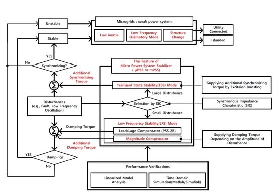
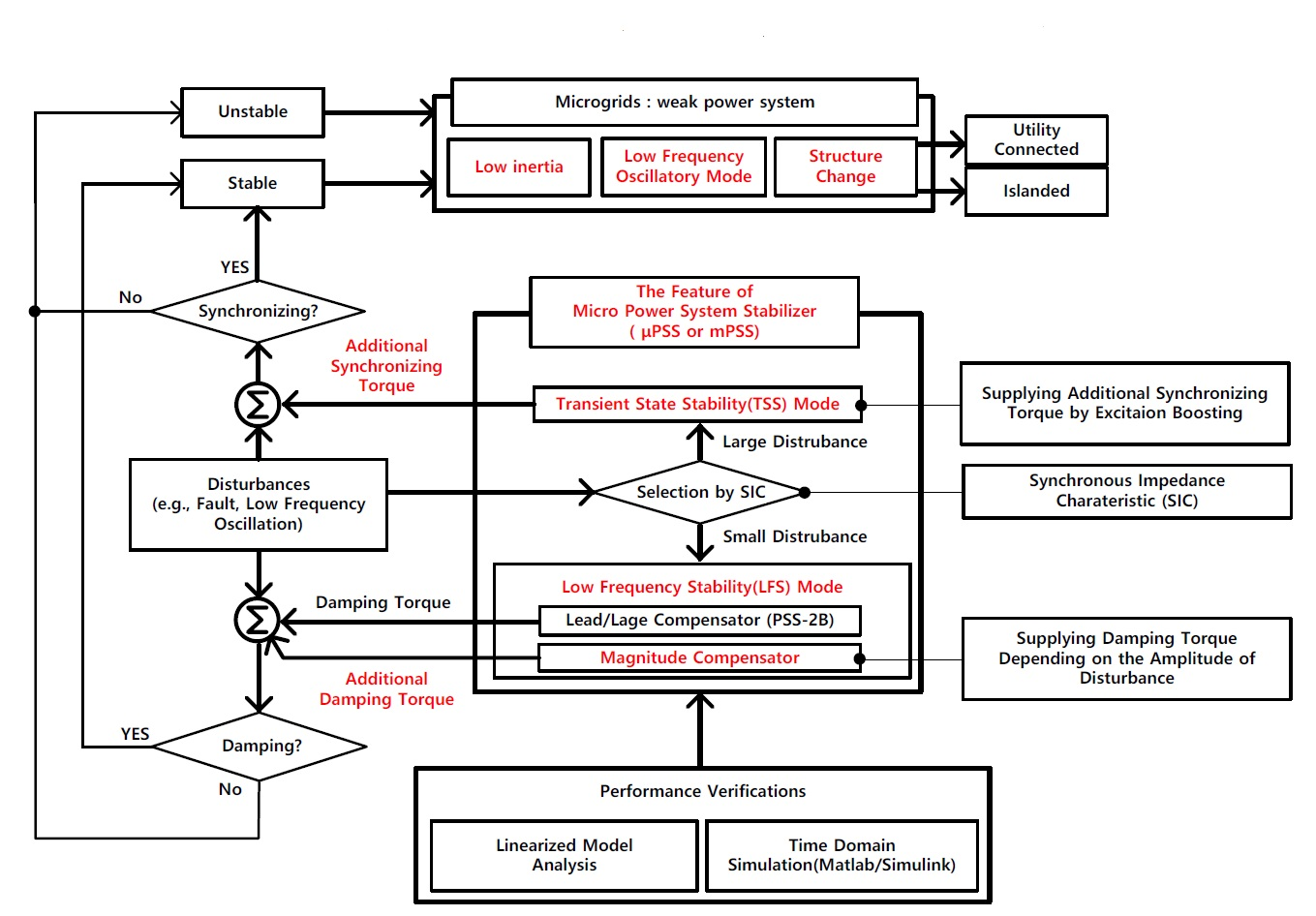
3. Proposed Power System Stabilizer for Stability Enhancement in Microgrids

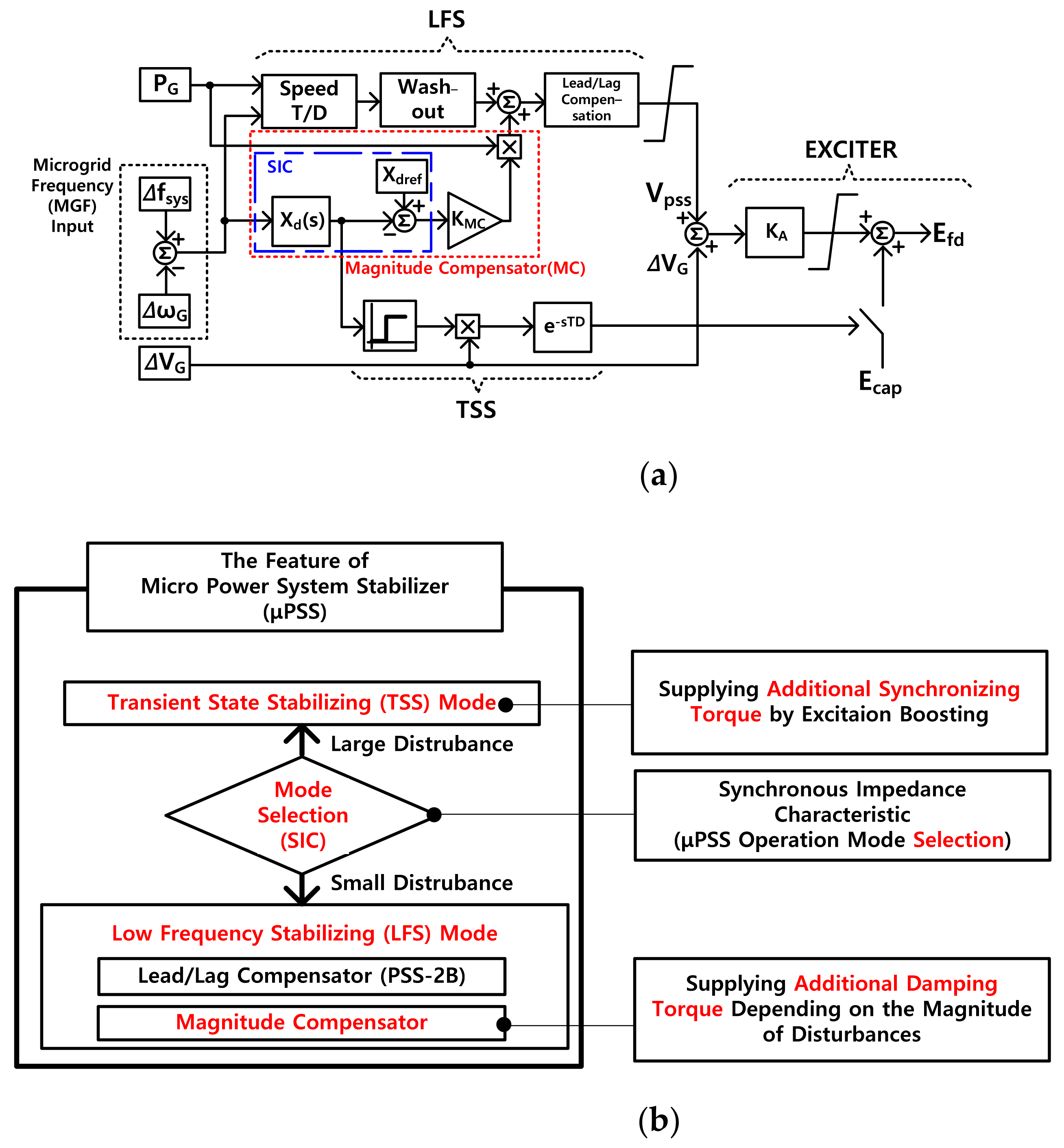
A micro-power system stabilizer ($\mathsf{\mu }$PSS) is designed to cope with structural changes in the microgrid, provide damping torque to low-frequency oscillations, improve the transient stability by supplying synchronizing torque under large disturbances. It also has the ability to automatically switch into low-frequency stabilizing (LFS) mode and transient state stabilizing (TSS) mode, depending on the amplitude of the SG’s swing.

As mentioned in Section 2, detection of the operating mode is necessary to cope with the variable structural characteristics of the microgrid. To detect the islanded operation, a method that relies on auxiliary signals, such as on/off contacts of a circuit breaker, is not suitable for distributed control and is not desirable for use due to concerns originated from the loss of the state signals. A suitable signal to add to the PSS is the frequency of the power system (i.e., microgrid frequency (MGF)). If the microgrid frequency is used as an input value, the additional signal plays a little role because the microgrid frequency is almost constant when the microgrid is in utility-connected operation mode. However, in the case of islanded operation, the added frequency signal is the target frequency for which the PSS provides damping torque as a criterion for the change in the rotational speed of the generator, as defined in the non-stiff system swing equation (Equation (8)), because frequency variation depends on the inertia of the microgrid in question.

The microgrid frequency can be easily obtained through a potential transformer, and the excitation system is always monitoring the voltage, so no additional devices are required. Therefore, adding the frequency signal of the power system to the input signal of the PSS enables enhancing the performance of the PSS to be enhanced regardless of the microgrid’s operation mode.

3.1. The Effects of Adding a Microgrid Frequency Signal to the Input of the PSS

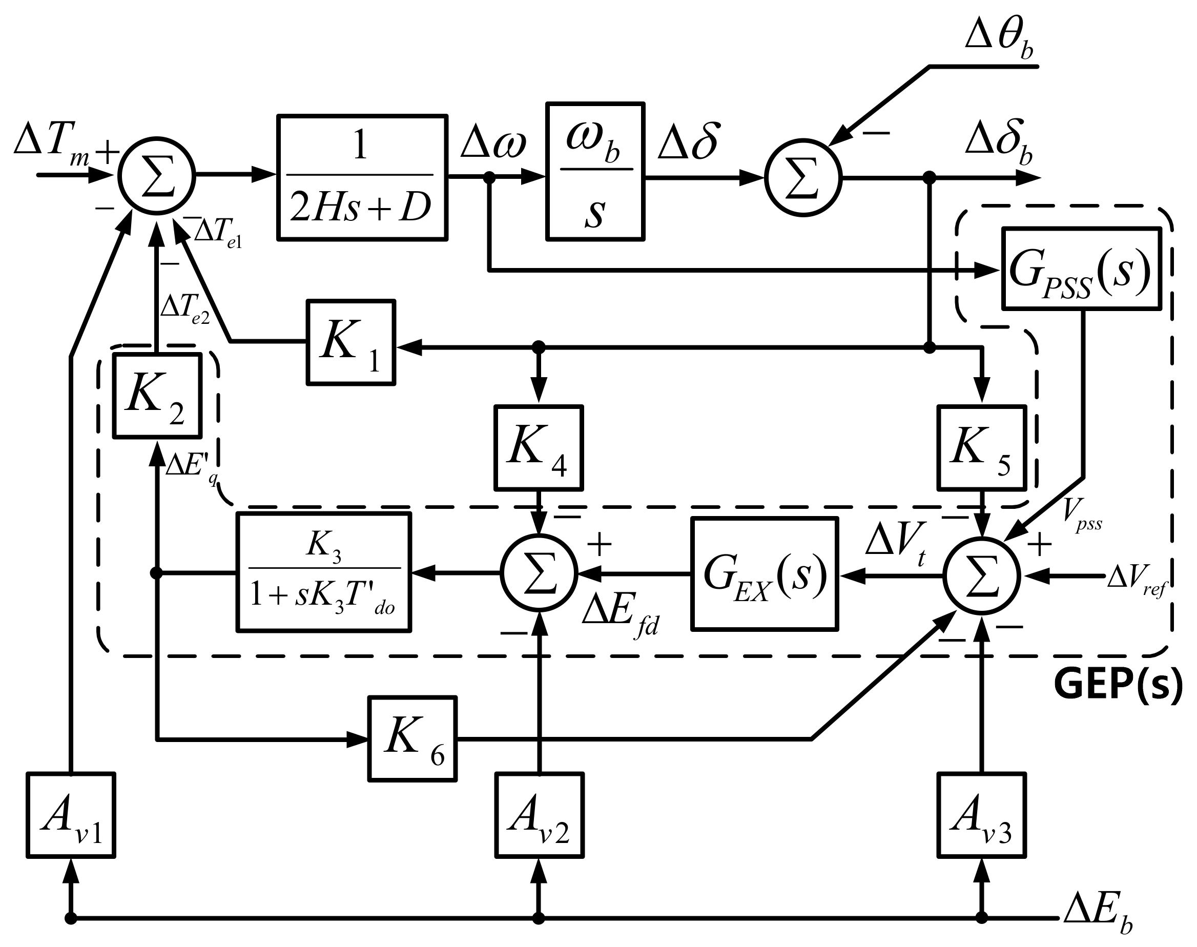
When a disturbance occurs in the microgrids in islanded mode, the system frequency and the rotational speed of the SG change. A $\mathsf{\mu }$PSS attenuates frequency variation because it damps an oscillation corresponding to a difference between two frequencies and performs phase compensation. To analyze the effects of using a microgrid frequency as an input, the following generator-exciter-PSS (GEP) model is used to analyze the damping effect by comparing the output differences depending on the two types of inputs.

$$GEP\left(s\right)=\frac{G_{PSS}\left(s\right)K_2{K}_A{K}_3}{K_A{K}_3{K}_6+\left(1+s{K}_3{T}_{do}^{\prime }\right)\left(1+s{T}_A\right)}=\frac{\Delta T_{pss}}{\Delta {\mathsf{\omega }}_{pss}}$$

$$\Delta V_{ref}=0, \Delta \delta =0, \mathrm{and} \mathrm{damping} \mathrm{torque}=\Delta T_{PSS}$$

$$GEP\left(s\right)\approx \frac{K_2}{K_6}\frac{G_{PSS}\left(s\right)}{\left(1+\frac{s{T}_{do}^{\prime }}{K_A{K}_6}\right)\left(1+s{T}_A\right)}=D_{MP}$$

(15)

If the PSS sufficiently compensates for the phase delay in the SG and the excitation system, the $D_{MP}$ becomes pure damping torque. In such a case, the characteristic equation of the SG is shown as follows [41]:

$$\frac{2H}{{\omega }_0}s\Delta {\omega }_G+D_{MP}\Delta {\omega }_G+K_1\frac{1}{s}\left(\Delta {\omega }_G-\Delta {\omega }_{MG}\right)$$

$$=s^2\Delta {\delta }_G+s\frac{D_{MP}}{M}\Delta {\delta }_G+\frac{K_1}{M}\left(\Delta {\delta }_G-\Delta {\delta }_{MG}\right)$$

$$=s^2+s\frac{D_{MP}}{M}+\frac{K_1}{M}-\frac{K_1}{M}\frac{\Delta {\delta }_{MG}}{\Delta {\delta }_G}=s^2+s\frac{D_{MP}}{M}+\frac{{K^{\prime }}_1}{M}$$

$$s_{1,2}=-\frac{D_{MP}}{2M}\pm j\sqrt{{\left(\frac{{K^{\prime }}_1}{M}\right)}^2-{\left(\frac{D_{MP}}{2M}\right)}^2}=-\xi {\omega }_n\pm j{\omega }_n\sqrt{1-{\xi }^2}$$

(16)

$$\frac{D_{MP}}{2M}=\xi {\omega }_n, \xi =\frac{D_{MP}}{2\sqrt{M{K^{\prime }}_1}}, D_{MP}=2\xi {\omega }_{n}M$$

As shown in the above results, adding the frequency signal of the microgrid to the input of the PSS causes $K_1>{K^{\prime }}_1$, which can improve the damping ratio (ξ) and cope with the system’s inertia changes when the operation mode of microgrids is changed.

3.2. Low-Frequency Stabilizing Mode

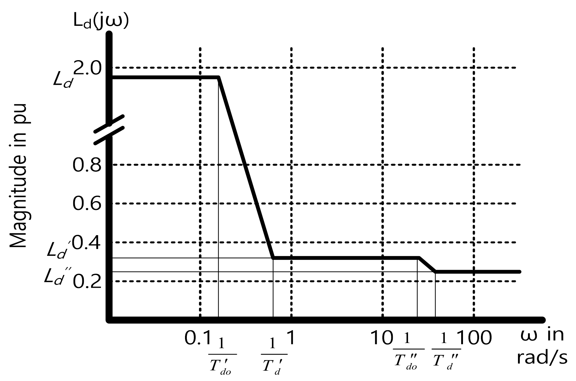
The general shape of the frequency characteristic applies to any synchronous machine [8]. The effective inductance is equal to the synchronous inductance, $L_d$, at a frequency less than 0.2 Hz; the transient inductance, ${L_d}^{\prime }$, in the range 0.2 Hz to 2 Hz; and the sub-transient inductance, ${L_d}^{″}$, 10 Hz or more. The characteristic of $L_d\left(s\right)$ can be expressed as the Equation (17) and Figure 2.

$$L_d\left(s\right)=L_d\frac{\left(1+s{T}_d^{\prime }\right)\left(1+s{T}_d^{″}\right)}{\left(1+s{T}_{do}^{\prime }\right)\left(1+s{T}_{do}^{″}\right)}$$

(17)

Since synchronous impedance is the same as the transfer impedance between the SG and the power system, frequency variation causes impedance changes and affects the power output, $P_e$, depending on Equation (1). This causes the perturbation of the rotor of the SG (i.e., swing), and the magnitude of the swing is determined in accordance with $\Delta P_e$. Given these characteristics, $X_d\left(s\right)$ in a PSS, the magnitude of the stabilization signal, can be controlled according to the magnitude of the perturbation (i.e., the required damping torque by the PSS) that should be compensated according to the frequency of vibration, thereby maximizing the effect of the oscillation damping.

The effect of a change in synchronous impedance on the SG’s power output is:

$$P_e=\frac{EV}{X_d}sin{\delta }_G$$

(18)

$$\frac{\partial P_e}{\partial X_d}=\frac{-EVsin{\delta }_G}{X_d^2}=\frac{-X_d^{0}EVsin{\delta }_G}{X_d^2·X_d^0}=-\frac{X_d^0}{X_d^2}{P}_e^0$$

(19)

super-scrip 0: initial value

When the generator power output differentiates concerning synchronous impedance, the correlation between synchronous impedance and the SG output deviation, Equation (19), can be obtained. Converting the torque of Equation (1) into effective power, we get the following:

$$T_m-T_e\approx \frac{P_m-P_e}{{\omega }_0}=P_m-P_e=2H\frac{d{\omega }_G}{dt}=M\frac{d{\omega }_G}{dt}$$

(20)

$$M\triangleq \frac{H}{\pi f_0}$$

The partial derivative of Equation (20) by synchronous impedance, $X_d$, is Equation (21), and substituting Equation (19) for Equation (21), the relation between the angular acceleration and the synchronous impedance, Equation (22), can be achieved.

$$\frac{\partial P_m}{\partial X_d}-\frac{\partial P_e}{\partial X_d}=M\frac{\partial }{\partial X_d}\left(\frac{d{\omega }_G}{dt}\right)$$

(21)

$$In case of P_m constant,$$

$$\frac{\partial {\alpha }_G}{\partial X_d}=\frac{1}{M}\frac{X_d^0}{X_d^2}{P}_e^0=\frac{1}{M}\frac{EVsin{\delta }_G}{X_d^2}$$

(22)

To replace the angular acceleration caused by the deviation of synchronous impedance with the acceleration torque of the rotor, from the swing equation (Equation (1)), we get

$$\frac{\partial T_{\alpha }}{\partial {\alpha }_G}=2H$$

(23)

Then, multiplying Equation (22) by Equation (23), chain rule,

$$\frac{\partial {\alpha }_G}{\partial X_d}·\frac{\partial T_{\alpha }}{\partial {\alpha }_G}=\frac{\partial T_{\alpha }}{\partial X_d}$$

(24)

The relationship between the synchronous impedance variation and the acceleration torque can be obtained, as shown in the following:

$$\frac{\partial T_{\alpha }}{\partial X_d}=\frac{EVsin{\delta }_G}{X_d^2}=\frac{P_G}{X_d}$$

$$\Delta T_{\alpha }=\frac{X_d^0}{{\mathrm{X}}_{\mathrm{d}}^2}{P}_e^0\Delta X_d=P_G\frac{\Delta X_d}{X_d}$$

(25)

Using the frequency characteristic of the SG (Equation (17)), the deviation of synchronous impedance (i.e., synchronous impedance characteristic) is obtained:

$$\Delta L_d\left(s\right)=L_d\left(1-\frac{\left(1+s{T}_d^{\prime }\right)\left(1+s{T}_d^{″}\right)}{\left(1+s{T}_{do}^{\prime }\right)\left(1+s{T}_{do}^{″}\right)}\right)$$

(26)

$$\Delta X_d=\left({\omega }_0+\Delta \omega \right)\Delta L_d\left(s\right)\approx {\omega }_0\Delta L_d\left(s\right)=\Delta L_d\left(s\right)$$

$$\frac{\Delta L_d}{L_d}=\left(1-\frac{\left(1+s{T}_d^{\prime }\right)\left(1+s{T}_d^{″}\right)}{\left(1+s{T}_{do}^{\prime }\right)\left(1+s{T}_{do}^{″}\right)}\right)\triangleq SIC\left(s\right)$$

(27)

Substituting Equation (27) for Equation (25) results in a correlation Equation (28) of acceleration torque with respect to the variation of frequency.

$$\Delta T_{\alpha }=P_G\left(1-\frac{\left(1+s{T}_d^{\prime }\right)\left(1+s{T}_d^{″}\right)}{\left(1+s{T}_{do}^{\prime }\right)\left(1+s{T}_{do}^{″}\right)}\right)$$

(28)

Applying Equation (28) as a control law of the magnitude compensation in the PSS can cancel out the acceleration torque generated by the frequency variation. In other words, the damping torque in the range of electro-mechanical mode can be selectively enhanced by compensating the magnitude of the SG’s swing or oscillation as well as phase compensation according to frequency variation, which is the fundamental function of the generic PSS. By adding a magnitude compensator (MC) to the generic PSS for configuring the controller, we can obtain the transfer function of the micro-power system stabilizer (Equation (29)) as follows:

$$\left(1-\frac{\left(1+s{T}_d^{\prime }\right)\left(1+s{T}_d^{″}\right)}{\left(1+s{T}_{do}^{\prime }\right)\left(1+s{T}_{do}^{″}\right)}\right)\triangleq SIC\left(s\right), MC\left(s\right)\triangleq P_G·\left|SIC\left(s\right)\right|$$

$$\mu PSS\left(s\right)=WO\left(s\right)\left(1+MC\left(s\right)\right)PC\left(s\right)$$

(29)

where

• $MC\left(s\right)$: magnitude compensator,
• $P_G$: generator active power output,
• $SIC\left(s\right)$: synchronous impedance characteristic,
• $WO\left(s\right)$: washout block, and
• $PC\left(s\right)$: phase compensator (i.e., lead-lag compensator).

It is a structure in which the input (i.e., frequency signal) is compensated by the MC after being filtered to a range of the selective frequency by the washout block of the transfer function (Equation (29)), and the signal is compensated through the lead-lag compensator to perform the phase compensation.

3.3. Transient State Stabilizing Mode

The transient state stabilizing (TSS) mode is added to prepare for large disturbances such as power system faults. This is based on the Lyapunov energy function, which is utilized for enhancing the transient stability of the SG [41,42,43,44]. The TSS control determines whether to perform an excitation boosting (EB) control, depending on the severity of disturbances. The EB provides instantaneously additional voltage of the charged capacitor to the field circuit, and this control strategy has been established and validated in [45,46]. Based on the EB control strategy, it integrates with the μPSS, considering the characteristics of microgrids.

3.3.1. Construction of the TSS Control Law

From [46], the Lyapunov energy function of the power system is defined as follows:

$$V=\frac{1}{2}{\displaystyle \sum }_{k=1}^{n}2H_k{\tilde{\omega }}_k^2-{\displaystyle \sum }_{k=1}^n{P}_{mi,k}^0{\tilde{\delta }}_k-{\displaystyle \sum }_{k=1}^{n-1}{\displaystyle \sum }_{l=k+1}^n{C}_{kl}^{0}cos{\tilde{\delta }}_{kl}+C_0$$

(30)

The rotor angle, ${\tilde{\delta }}_k$, and speed, ${\tilde{\omega }}_k$ are:

$${\tilde{\delta }}_k={\delta }_k-{\delta }_{COI}, {\tilde{\omega }}_k={\omega }_k-{\omega }_{COI}, { \mathsf{\omega }}_{COI}=\frac{{{\displaystyle \sum }}_{i=1}^N{H}_i{\omega }_i}{{{\displaystyle \sum }}_{i=1}^N{H}_i}$$

(31)

where the net internal mechanical power, $P_{mi,k}$, is expressed as a function of the mechanical power, $P_{m,k}$, the network equivalent shunt conductances, $g_{kk}$, and the voltage behind the transient reactance, $E_k^{\prime }$:

$$P_{mi,k}=P_{m,k}-g_{kk}{E}_k^{\prime }{}^2$$

(32)

In the controlled system,

$$\frac{dV}{dt}=\nabla V·f\left(x\right)+\nabla V·g\left(x\right)·u=\frac{d{V}_{unctrl}}{dt}+\frac{d{V}_{ctrl}}{dt}$$

$$=0+\left[{\displaystyle \sum }_{k=1}^n\left(\Delta P_{mi,k}-{\displaystyle \sum }_{l=k+1}^n\Delta C_{kl}sin{\tilde{\delta }}_{kl}\right){\tilde{\omega }}_k\right]$$

(33)

$$\Delta P_{mi,k}=-g_{kk}\left(2E_k^{\prime 0}\Delta E_k^{\prime }+\Delta E_k^{\prime 2}\right), \Delta C_{kl}=\left[\left(E_k^{\prime 0}+\Delta E_k^{\prime }\right)\left(E_l^{\prime 0}+\Delta E_l^{\prime }\right)-E_k^{\prime 0}{E}_l^{\prime 0}\right]b_{kl}$$

$$E_k^{\prime }\approx K{E}_{fd,k}, E_k^{\prime }=E_k^{\prime 0}+\Delta E_k^{\prime }$$

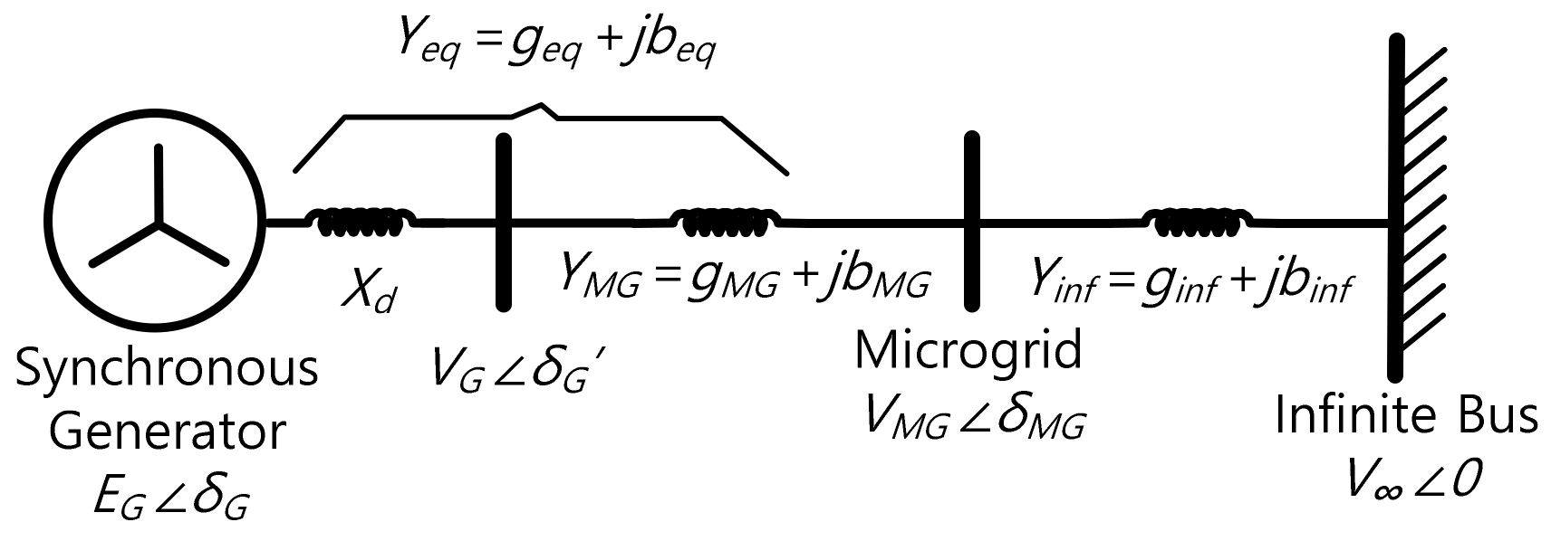
To modify the above Equation (33) to fit the features of the microgrid, we redefine variables using the following Figure 3.

$E_i^{\prime }$ of the other SG of the power system can be seen equivalent to $V_{MG}^{\prime }$ of the microgrid, and the transfer admittance is equal to the equivalent admittance, $Y_{eq}$, between the internal electromotive force, $E_G$, of the SG and the microgrid voltage, $V_{MG}$.

$$E_k^{\prime }\approx K{E}_{fd,k},$$

$$E_k^{\prime }=E_G=E_G^0+\Delta E_G, E_l^{\prime }=V_{MG}^0+\Delta V_{MG}$$

(34)

${\omega }_{COI}$ of Equation (31) is the calculated value of ${\omega }_i$ of the i-th SG measured using the phasor measurement unit (PMU) and the wide-area measurement system (WAMS). The microgrid is a distributed control system based on the plug-and-play concept, and it is desirable not to use additional communication devices. It is advantageous to utilize the frequency of the generator terminal voltage through the potential transformer (PT) rather than calculating the center of inertia using the WAMS. Therefore, ${\omega }_{COI}$ and ${\delta }_{COI}$ signals are replaced by ${\mathsf{\omega }}_{MG}$ and ${\mathsf{\delta }}_{MG}$, which do not require networks (e.g., WAMS), as shown below.

$${\omega }_k={\omega }_G, {\delta }_k={\delta }_G$$

$${\omega }_{COI}\approx 2\pi f_{MG}\triangleq {\omega }_{MG}, {\delta }_{COI}\approx {\delta }_{MG}$$

$${\omega }_G-{\omega }_{MG}\triangleq {\tilde{\omega }}_G, {\delta }_k-{\delta }_{MG}\triangleq {\tilde{\delta }}_G$$

(35)

Using Equations (34) and (35) in Equation (33), we have

$${\displaystyle \sum }_{k=1}^n\Delta P_{mi,k}=-g_{eq}\left(2E_G^{\prime 0}\Delta E_G+\Delta E_G^2\right)$$

$${\displaystyle \sum }_{k=1}^n{\displaystyle \sum }_{l=k+1}^n\Delta C_{kl}sin{\tilde{\delta }}_{kl} = -\left[\left(E_G^0+\Delta E_G\right)\left(V_{MG}^0+\Delta V_{MG}\right)-E_G^0{V}_{MG}^0\right]b_{eq}sin{\tilde{\delta }}_G$$

$$\frac{dV}{dt}=-g_{eq}\left(2E_G^0\Delta E_G+\Delta E_G^2\right){\tilde{\omega }}_G-\left[\left(E_G^0+\Delta E_G\right)\left(V_{MG}^0+\Delta V_{MG}\right)-E_G^0{V}_{MG}^0\right]b_{eq}sin{\tilde{\delta }}_G{\tilde{\omega }}_G$$

$$\approx -{\tilde{\omega }}_G\left\{\begin{array}{c}{g}_{eq}\left(2E_G^0\Delta E_G+\Delta E_G^2\right)\\ +\left(\Delta E_G\left(1-\left|\Delta V_{MG}\right|\right)-E_G^0\left|\Delta V_{MG}\right|\right)b_{eq}sin{\tilde{\delta }}_G\end{array}\right\}$$

(36)

$$0\le \left|\Delta V_{MG}\right|\le 1, g_{eq}<b_{eq}$$

Therefore, if Equation (36) is negative, the system can go back to the equilibrium point. When the system voltage drops under large disturbances, the power system will have the following conditions:

$$E_G^0>\Delta E_G, 0\le \Delta V_{MG}\le 1$$

$$\Delta E_G\left(1-\left|\Delta V_{MG}\right|\right)<E_G^0\left|\Delta V_{MG}\right|$$

(37)

Because the microgrid’s admittance is relatively insignificant compared to the synchronous impedance, the following conditions are established:

$$\Delta V_{MG}\approx \Delta V_G, \frac{1}{Y_{MG}}\ll X_d$$

(38)

Therefore, the SG can return to the equilibrium point under the Lyapunov energy function if ${\tilde{\omega }}_G>0, \Delta E_G^{\prime }>0$ is maintained until the following conditions are met:

$$\Delta E_G\left(1-\left|\Delta V_{MG}\right|\right)\ge E_G^0\left|\Delta V_{MG}\right|$$

(39)

The control strategy to satisfy the above conditions in TSS mode can be established as follows:

$$V_{TSS}=K_{TSS}{\tilde{\omega }}_G\left|\Delta V_G\right|$$

(40)

TSS mode is a method of momentarily injecting the booting voltage directly into the field circuit bypassing the AVR circuit. TSS mode determines the injection period, starting point, and end point by Equation (40). Some circuit modifications and installation of additional facilities are required, as additional capacitance and switches need to be configured. It can increase the synchronizing power strongly due to a momentary increase in the field voltage, which also improves the transient stability.

TSS mode should be used in a very limited manner, as features that directly affect the field voltage have an enormous impact on the stability of the SG. The method in [46] calculated the center of inertia (COI), ${\omega }_{COI}$, in real time using the WAMS and improved the accuracy of EB motion through the relative generator speed, ${\omega }_G$, for ${\omega }_{COI}$. In a $\mathsf{\mu }$PSS, ${\omega }_{MG}$ does not have the exact same value as ${\omega }_{COI}$, so it can affect the selectivity of the EB action according to Equation (36). Therefore, to overcome some of the deficient selectivity, a synchronous impedance characteristic (SIC) is used to provide highly reliable selectivity so that LFS and TSS modes can operate and coexist depending on the circumstances facing the situation of the SG, as will be described in Section 3.4.

3.3.2. The Specifications of Boosting Capacitance

Boosting capacitance (BC) is modeled as an ideal capacitor whose voltage, $E_{cap}$, is determined by the maximum field voltage that the rotor can withstand with a security margin [46]. Given the maximum allowable field voltage (limited by the rotor winding insulation), $E_{fdLim}$, the DC ceiling voltage (maximum DC voltage produced by the rectifier), $E_{fdMax}$, and the generator terminal voltage, $V_G$, the capacitor voltage are determined as:

$$E_{cap}\le E_{fdLim}-E_{fdMax}·V_G$$

(41)

Within the allowed insulation of the field circuit, setting the maximum operating hours, $t_{BC}$ and $E_{cap}$, offers $C_{BC}$ of the BC.

$$C_{BC}\left[F\right]=t_{BC}\left[s\right]·\frac{I_{fdBase}}{E_{fdBase}}$$

(42)

3.4. Mode-Switching Condition: LFS ← Selection → TSS

Generally, damping torque is enhanced by the PSS, but synchronizing torque could be reduced in part [12]. To overcome these shortcomings, a $\mathsf{\mu }$PSS needs to have appropriate transitions between modes so that it can operate in LFS mode in the range of low frequency and in TSS mode in transient conditions under large disturbances. A $\mathsf{\mu }$PSS can take advantage of the high-gain excitation system and overcome shortcomings by increasing synchronizing torque through the TSS and the supply of damping torque through the LFS. For the two modes to coexist, the synchronous impedance variation (i.e., SIC) of the SG is used as the mode selection signal. Because the deviation in synchronous impedance is proportional to the disturbance’s size, this signal can be used to ensure that the $\mathsf{\mu }$PSS operates in the appropriate mode, depending on the situation in the microgrid.

Synchronous impedance is an electro-magnetic phenomenon that can be modeled as impedance, which is changed by the variation of the rotational speed of the SG. Frequency characteristics of synchronous impedance can be obtained with the machine’s parameters [8], which can be used to estimate the amplitude of the swing. These synchronous impedance frequency characteristics can be used as the basis for switching between TSS mode, which increases synchronizing torque for transient stability, and LFS mode, which provides LFOs with damping torque.

4. Features of the Proposed $\mathsf{\mu }$PSS

The $\mathsf{\mu }$PSS is based on the structure of PSS-2B and is a form with the addition of a transient state stabilizing (TSS) loop, a magnitude compensator (MC), and a synchronous impedance characteristic (SIC) function. The MC adjusts the magnitude of the compensation signal by considering the sensitivity between the angular acceleration and torque variation for frequency variation and utilizes an SIC as a reference signal for selecting LFS or TSS mode, providing selectivity. The TSS serves to improve synchronizing torque by providing an initiation signal to temporarily boost the field voltage in a transient state. The overall structure of the $\mathsf{\mu }$PSS is shown in Figure 4.

The main functions of each block and structural features of the $\mathsf{\mu }$PSS compared to PSS-2B (see Figure A1) are as follows.

4.1. Microgrid Frequency (MGF) Input Signal

$\Delta f_{sys}$ and $\Delta {\omega }_G$ are used as inputs to cope with the low inertia of the system as the system switches to islanded operation. These inputs are used as a reference of the oscillation, which is damped by the $\mathsf{\mu }$PSS, between the system frequency and rotor angle of the SG.

4.2. Low-Frequency Stabilizing (LFS) Mode

The $\mathsf{\mu }$PSS is a form with the addition of a magnitude compensator (MC) to PSS-2B, and it provides damping torque for LFOs, depending on the amplitude of the swing (e.g., oscillations). Other parts are based on the structure of PSS-2B, which shows the most stable performance among various structures such as a conventional PSS, PSS-2B, and PSS-4B [9,10,47,48]. Thus, the general characteristics of the LFS are identical to those of PSS-2B and show a greater oscillation suppression effect as a result of the improvement in the gain in the range of low frequency by the MC. From now on, PSS-2B will be called gPSS, unless otherwise noted.

4.3. Magnitude Compensator (MC) Block

In addition to the phase compensation by the lead-lag compaction block of the gPSS in LFS mode, the MC performs magnitude compensation. Because synchronous impedance changes produce acceleration torque, the relationship between frequency and acceleration torque according to Equation (28) allows this function to be compensated for the output signal ($V_{pss}$) of the LFS of the $\mathsf{\mu }$PSS.

4.4. Synchronous Impedance Characteristic (SIC) Block

Through the relationship between frequency and impedance change according to synchronous impedance characteristics (SICs), Equation (27), the SIC block extracts the magnitude of the disturbance. Using this method, LFS and TSS modes are selected according to the situation at hand and are also utilized to perform the MC, as described above.

5. Tuning the Parameters of the $\mathsf{\mu }$PSS for Verifications

The PSS compensates for the phase delay caused by the characteristics of the excitation system and field circuit through lead-lag compensators. The parameter is a critical factor in determining the PSS’s performance, because the inaccurate parameter can amplify the generator’s rotational oscillations. Therefore, it is necessary to select a more objective tuning method for parameters to accurately identify and verify the performance, characteristics, and effects of the $\mathsf{\mu }$PSS proposed in this paper.

The $\mathsf{\mu }$PSS consists of parameters in PSS-2B: the SIC, MC, and TSS. Because the SIC, MC, and TSS are dependent parameters determined by the characteristics of the SG, the tuning of the $\mathsf{\mu }$PSS can be performed in the same way as that of PSS-2B.

The tuning methods of a PSS typically include the traditional one [49,50] that is performed by the procedure of the guide using the analytical technique of control theory and one that utilizes the heuristic optimization algorithm (HOA) that is used in various fields [7,20,21,22,23,24]. It is judged that utilizing heuristic optimization based on algorithms that perform objective function optimization would be more suitable for the performance verification of the $\mathsf{\mu }$PSS than traditional methods, which are often influenced by the experience, ability, and intuition of the engineer. Therefore, the tuning of the $\mathsf{\mu }$PSS will be performed through particle swarm optimization (PSO), which is widely used as a PSS parameter-tuning method due to its outstanding performance among HOAs [2,18]. The objective function of PSO is the following Equation (43), which is widely used in PSS tuning, and the parameter of the objective function is set up as

Table 3. PSO parameter setting.

Particle	7
Population	10 × 7
Inertia range	0.1–1.1
Max. iterations	100 × 7
${\sigma }_0$	−2.5
${\zeta }_0$	0.1
$\alpha$	15

and using the D-shaped sector in Figure 5 [21,23].

$$E={\displaystyle \sum }_{{\sigma }_i\ge {\sigma }_0}{\left({\sigma }_0-{\sigma }_i\right)}^2+\alpha {\displaystyle \sum }_{{\zeta }_i\ge {\zeta }_0}{\left({\zeta }_0-{\zeta }_i\right)}^2$$

(43)

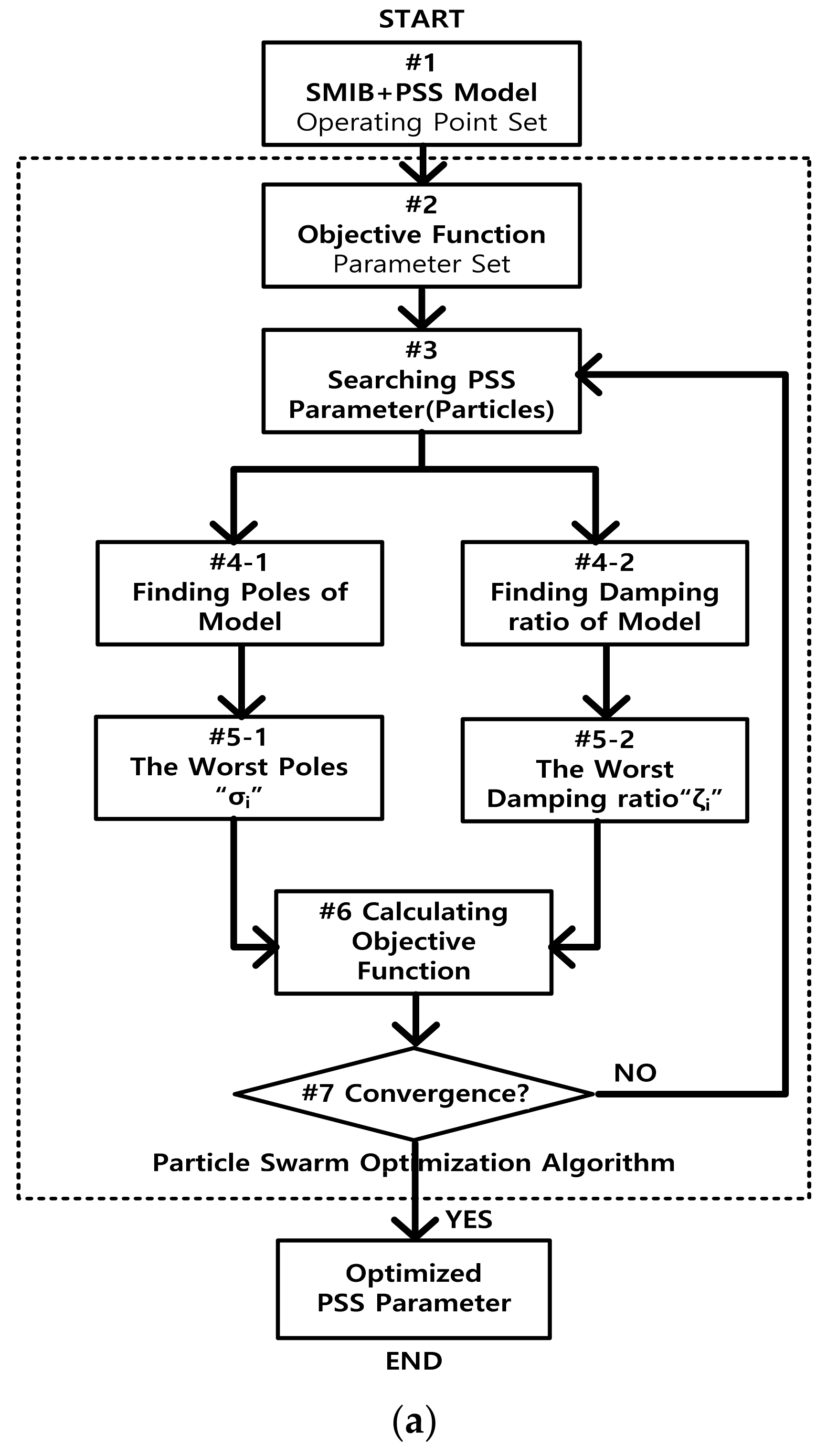
PSO optimizes the parameters of the PSS so that the worst pole and damping ratios of the single-machine non-stiff bus (SMNB) model, which is linearized by 10 operating points (see

Table A1. The 10 operating points of the synchronous generator for the SMNB model.

Operating Point	Vq	Vd	Eq	E′q	iq	id	$\mathit{\delta }$
1	0.9322	−0.3630	1.2059	1.0086	0.3424	−0.2582	0.4608
2	0.8882	−0.4589	1.2832	0.9985	0.4329	−0.3727	0.5975
3	0.7363	−0.6775	1.6722	0.9976	0.6392	−0.8829	0.9768
4	0.9988	−0.2080	1.0729	1.0195	0.1963	−0.0700	0.2485
5	0.8568	−0.6403	1.5683	1.0555	0.6041	−0.6712	0.8217
6	0.7918	−0.6100	1.4996	0.9894	0.5754	−0.6677	0.8445
7	0.8139	−0.5801	1.4799	0.9999	0.5473	−0.6282	0.7965
8	0.8914	−0.5561	1.7032	1.1181	0.5246	−0.7659	0.7413
9	0.8585	−0.6049	1.5719	1.0577	0.5707	−0.6730	0.7924
10	0.7712	−0.6039	1.4064	0.9486	0.5697	−0.5992	0.8442

), have values in the predefined range of the D-shaped sector. To utilize PSO for tuning, the setup for the optimization algorithm is required, and the relevant settings are summarized in the table.

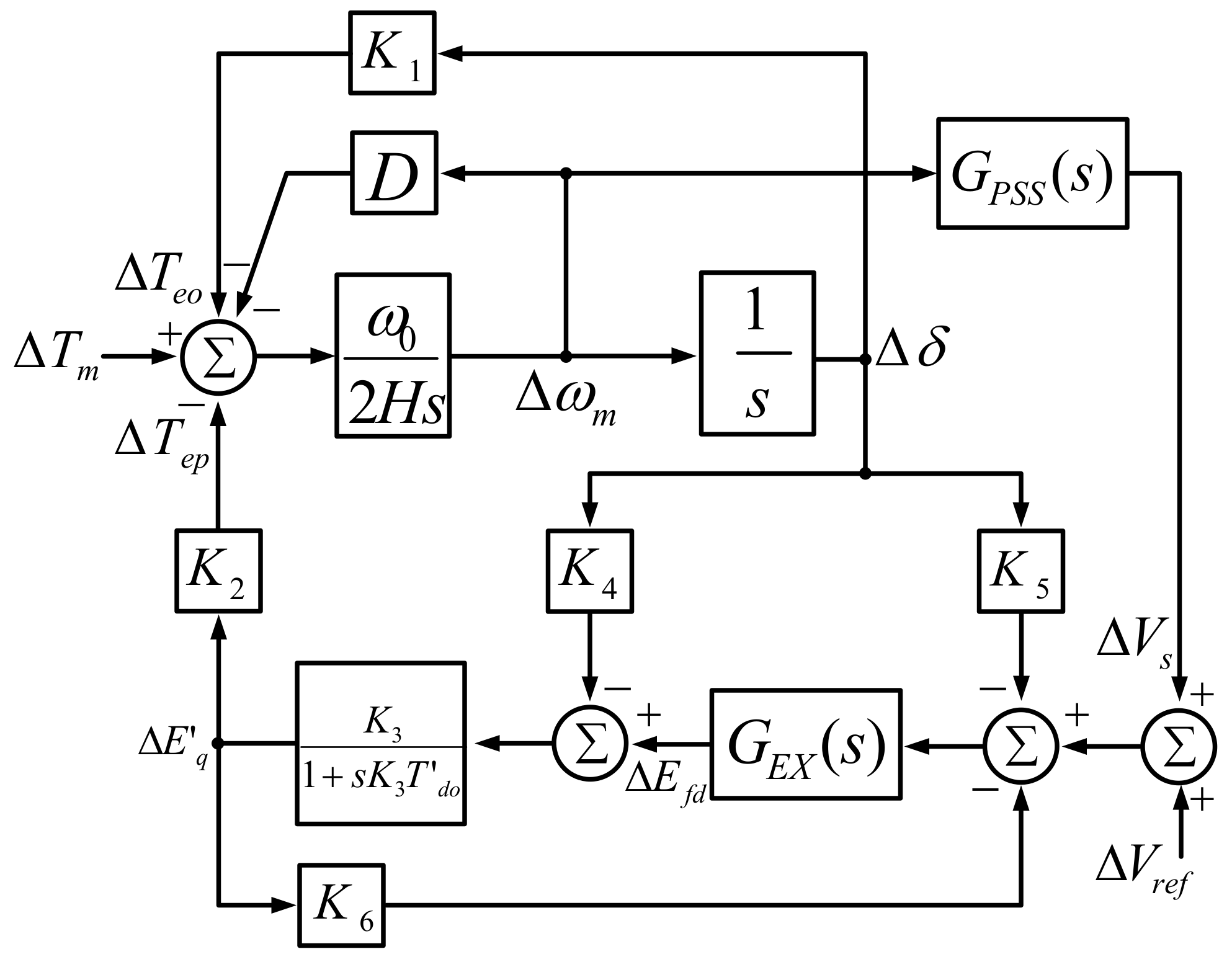
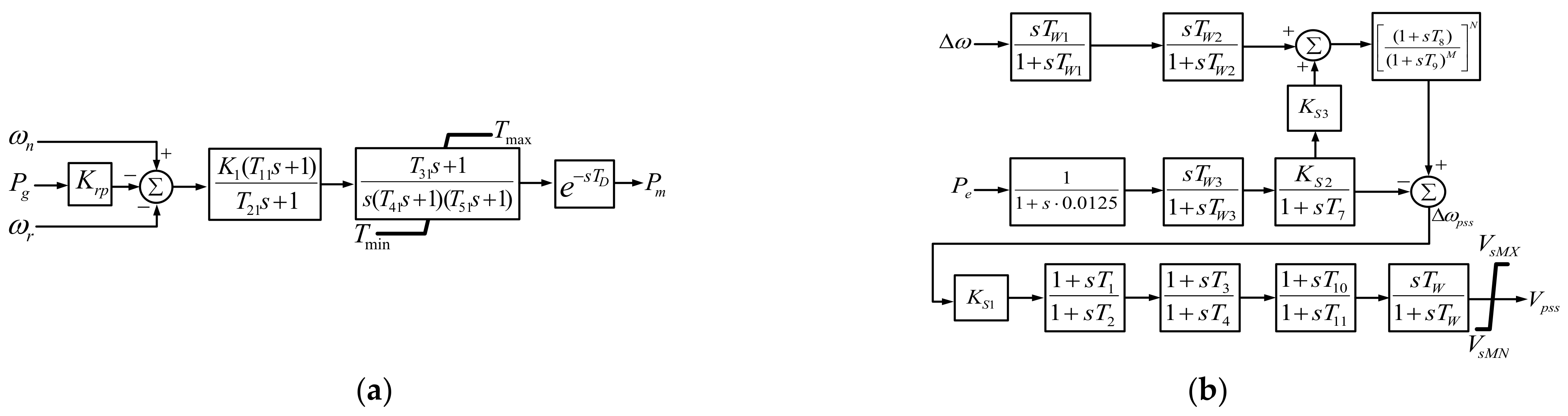
The optimization follows the procedure described in the Figure 7a flowchart, and 10 operating points of the SG are listed in Table A1. To perform optimization using PSO, linearized models of the SG and power systems are needed. Heffron-Philip’s model (HP model, Figure 1) is widely known as the K-constant model (i.e., SMIB) and has been used in a number of studies on PSS design [13,14,15,41,49,50]. The HP model, a representative one of the stiff voltage system, may be suitable for tuning the gPSS used in large power systems, but it is necessary to consider the effects of bus voltage fluctuations in tuning the parameters of the $\mathsf{\mu }$PSS, which is operated in microgrids.

A single-machine non-stiff bus (SMNB) is a model that considers changes in the magnitude and phase of the connected power system voltage and is used to make up for the shortcomings of a conventional K-constant model [16,17]. Therefore, the use of the SMNB model (see Figure 6) could consider the effects of the weak system in parameters of the μPSS, so PSO is performed with the model.

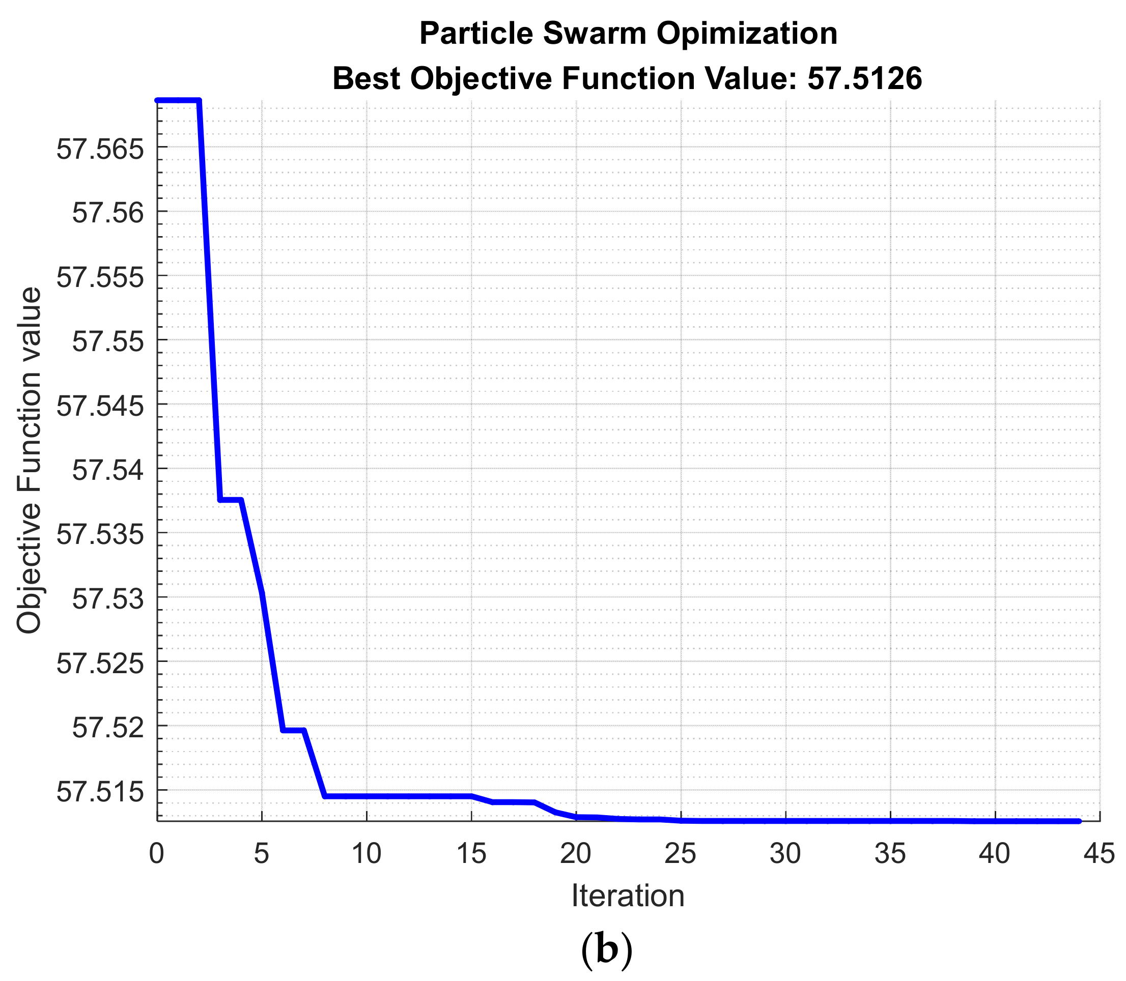
Parameters optimized through PSO are listed in

Table 4. Optimized parameters of the PSS for verifying the performance of the $\mathsf{\mu }$PSS.

Parameter	Range of Value [47]	Optimized Value Using PSO
KS1	1–50	50
T1	0.01–1.5	0.8963
T2	0.01–1.5	1.5
T3	0.01–1.5	0.8921
T4	0.001–1.5	1.5
T10	0–1	0.8894
T11	0–1	0
TW1 = TW2 = TW3 = 10; VS_MAX = −VS_MIN = 0.1; T7 = 2H;
M = 5; N = 1; T8 = 0.5; T9 = 0.1;
KS2 = 1 KS3 = 1 [10]

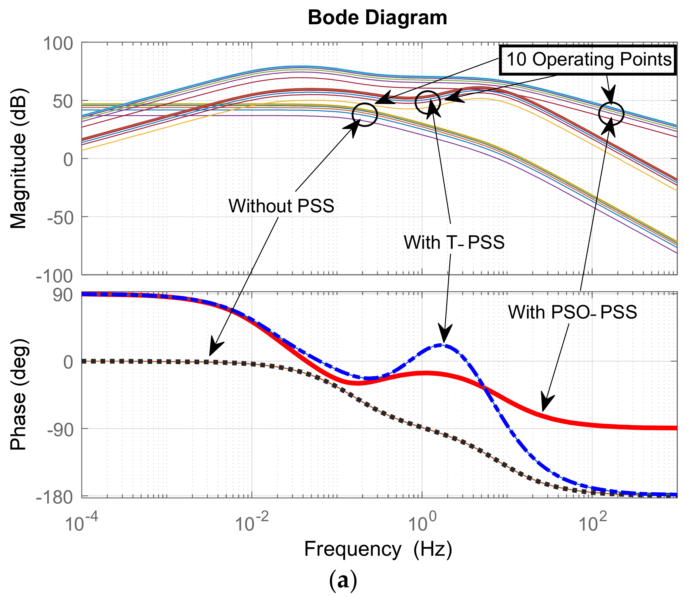
. As shown in Figure 7b, the value of the objective function is converged at the minimum by the PSO algorithm. In Section 7, we will validate these parameters by comparing and analyzing a PSO-optimized PSS (PSO-PSS), typical parameters of a PSS (T-PSS), and the case of an SG without a PSS (w/o PSS).

6. Stability Analysis

This section will verify the characteristics and performance of the $\mathsf{\mu }$PSS through small-signal stability analysis using the linearized model. Models that are linearized as an SMNB and GEP with 10 operating points (see

Table A2. Synchronous generator

Parameter	Setting Value
${\mathrm{X}}_{\mathrm{d}}$${{\mathrm{X}}_{\mathrm{d}}}^{\prime }$${{\mathrm{X}}_{\mathrm{d}}}^{″}$	1.56 0.296 0.177
${\mathrm{X}}_{\mathrm{q}}$${{\mathrm{X}}_{\mathrm{q}}}^{\prime }$${{\mathrm{X}}_{\mathrm{q}}}^{″}$	1.06 0.177 0.052
${{\mathrm{T}}_{\mathrm{d}}}^{\prime }$${{\mathrm{T}}_{\mathrm{d}}}^{″}$${{\mathrm{T}}_{\mathrm{qo}}}^{″}$	3.7 0.05 0.05
H pole-pairs	1.07 2

) are used for verification. Models of the location of the poles, frequency characteristics, and step response will be used to analyze in detail the stability of the system applying the $\mathsf{\mu }$PSS. The frequency characteristics will be checked by phase and magnitude characteristics by frequency input using the Bode diagram. In addition, the improvement effect of each mode of the system will be verified by checking the location of the pole, and the convergence of the SG angle under disturbances will be checked on the time axis through the step response.

Transient stability analysis is required to verify TSS mode, but linearized models cannot accurately analyze the effects under sudden change. Besides, analysis of the impact of the addition of a microgrid frequency input signal is also impossible using the SMNB model due to the nature of the linearized model, which is the single input single output system, in which two inputs cannot be used. Therefore, the above two characteristics of the $\mathsf{\mu }$PSS will be verified in Section 7 through a case study using time-domain simulation.

Before verifying the performance of the $\mathsf{\mu }$PSS, we will verify the effectiveness of parameters tuned by PSO.

6.1. Verification of the PSS Parameters Tuned by PSO

Prior to the performance verification of the $\mathsf{\mu }$PSS, the parameters of the PSS play a crucial role in performance, so analysis of parameters should be required. In this paper, both the gPSS and the $\mathsf{\mu }$PSS are tuned to the same parameters (i.e., tuned by PSO) to show the performance difference for the newly proposed structures of the $\mathsf{\mu }$PSS under the same conditions. Therefore, before analyzing the performance of the $\mathsf{\mu }$PSS and gPSS in earnest, we first verify the parameter-tuning results accomplished in Section 5. The analysis of efficacy on the detailed differences of parameters is outside the scope of this paper; instead, using control theory techniques, the overall stability of the SG will be analyzed to check the integrity of the parameters.

The change in electrical torque to the deviation of the frequency input through the GEP model can be seen in Figure 8. Comparing the gPSS tuned with PSO (PSO-PSS), PSS-2B with typical parameters (T-PSS), and the case without a PSS (w/o PSS), it can be determined that PSO-PSS, as in the Figure 8a Bode diagram, provides appropriate damping torque for the LFO, as shown in −90° phase characteristics. The SMNB model is the one with the input of difference between mechanical and electrical torque and with the output of angle change. In addition, it is conducive to gauge whether it can converge to a new steady state in oscillations caused by disturbances. Among the total 10 operating points, it can be seen that the poles of the PSO-PSS marked with red solid circles on the s-plane are all located in the left half-plane, contrasting with the two that are marked with blue dashed lines, and the case without a PSS in black dotted lines is located on the right half-plane. One notable point was that only the PSO-PSS can be found located on the left half-plane in the electro-mechanical mode, which occurs in the area of the purple box (near the border between the left and right half-planes) in Figure 8b. Given that the overall stability analysis shows significant stability improvement in the case of using a PSO-PSS, it can be concluded that the parameters tuned by PSO are optimized for the linearized model. From now on, we will proceed with the simulation using the PSS set by parameters optimized by PSO, unless otherwise noted.

6.2. Verification of the $\mu$PSS

Because the $\mathsf{\mu }$PSS is based on the PSS-2B structure, all parameters tuned by PSO can be shared with the $\mathsf{\mu }$PSS. The additional parameters needed to be set for the $\mathsf{\mu }$PSS are nearly all dependent on the machine parameters of the SG where the $\mathsf{\mu }$PSS is to be installed, except the weight parameters of the MC, ${\mathrm{K}}_{\mathrm{MC}}$, and the threshold parameters of the TSS. The characteristic of the $\mathsf{\mu }$PSS improving the gain only in the range of LFOs can be confirmed by the frequency characteristics in the Bode diagram and the pole locations in the s-plane.

Comparing the gPSS (PSS-2B) and the $\mathsf{\mu }$PSS using the GEP model, the magnitude of the GEP model with the $\mathsf{\mu }$PSS in the Bode diagram in Figure 9a shows that the $\mathsf{\mu }$PSS increases its magnitude over the limited frequency range (below 10 Hz) due to the effects of the MC block in the $\mathsf{\mu }$PSS. In other words, the PSS supplies damping torque in the frequency band where the SG is particularly vulnerable. Generally known frequency ranges are inter-machine mode (0.7–2.0 Hz), inter-area mode (0.1–0.3, 0.4–0.7 Hz), and inter-microgrid mode (3.4–6 Hz) [8,24], which shows the increased magnitude of the GEP(s). These characteristics of the $\mathsf{\mu }$PSS are the main factors that enable the $\mathsf{\mu }$PSS to perform better than the gPSS because they can provide greater damping torque in electro-mechanical mode, a frequency band of the range that is vulnerable to the stability of the SG.

Figure 9b shows the distribution of the overall poles of the SMNB with gPSS and $\mathsf{\mu }$PSS models. The areas marked with purple solid lines are particularly vulnerable to stability close to the boundary between the left and right half-planes on the s-plane, and a closer look at Figure 9c shows that the poles of the μPSS marked with red solid lines are located further to the left than those of the gPSS marked with blue dashed lines. As a result, the $\mathsf{\mu }$PSS supplies more enormous damping torque, which further enhances the stability of the system (i.e., SG) at all operating points.

The frequency-domain analysis of the SMNB and GEP models confirms that the SG with the $\mathsf{\mu }$PSS has a more stable performance. This time, we check the convergence of the SMNB according to the size of the step change in the time domain through the step response. A total of four operating points (#1, #3, #5, #7) are used to analyze whether $\Delta \mathsf{\delta }$ converges against $\Delta \mathrm{T}$ with a step response in the SMNB model. The size of the step is 0.3 and 0.6 each, and the black dotted line represents the system without a PSS (w/o PSS); the blue dashed line, the gPSS (PSS-2B); and the red solid line, the $\mathsf{\mu }$PSS. Results are shown in Figure 10a–h, and in most cases, the system without a PSS is unstable due to insufficient damping and the system with a μPSS shows the most stable response.

7. Case Study

Using the MATLAB/Simulink microgrid model (see Figure A2), we will verify and analyze the performance of the two kinds of μPSSs’ functions under various scenarios: one with TSS mode and the other with an MGF, which could not be checked in the linearized model. The μPSS supplies damping torque in LFS mode for LFOs and switches to TSS mode under large disturbances (e.g., phase short faults, ground fault, and so on), which perform EB control to improve synchronizing torque. Therefore, a minor reduction in synchronizing torque of the SG by the influence of the PSS can be sufficiently covered by TSS mode. The effect of TSS mode could not be verified in Section 6 because it was difficult to be included in the linearized model analysis. In this section, however, the effects of TSS mode will be verified through time-domain simulation (TDS). In addition, depending on whether the MGF input is used as a reference signal, the performance characteristics of the PSS will be checked. Finally, the comparative analysis of the performance of the μPSS and gPSS-2B under various disturbances will be used to determine the comprehensive excellence of the μPSS. Microgrid simulation models and detailed specifications of components are included in the Appendix A (see Figure A2 and

Table A5. Specification of a simulation model.

Components		Specification	Initial Loading in TDS	Remarks
Generation	SG #1 *	2 (MVA)	0.5 pu	With a μPSS
	SG #2 **	2 (MVA)	0.49 pu
	Photovoltaic #1 **	500 (kW)	1 pu
	Photovoltaic #2 **	700 (kW)	1 pu
Load	P-Q Load #1	500 (kW) + j240 (kvar)	Varying with case study scenario	Peak Load3 (MW) + j0.78 (Mvar)
	P-Q Load #2	400 (kW) + j190 (kvar)
	R-L Load #1	1100 (kW)+ j150 (kvar)
	R-L Load #2	1000 (kW) + j200 (kvar)
Network	Power Cable	0.01273 (Ω/km)	N/A
		0.9337 × 10−3 (H/km)
		12.74 × 10−9 (F/km)

* Model with a μPSS in TDS; ** fixed output.

).

7.1. Case Study #1: Differences between the gPSS with an MGF and the gPSS without an MGF

In accordance with Section 3.1, an MGF is used as input for the μPSS. This is a way to cope with the changes in the system’s inertia because of the structural changes in the microgrids. The $\mathsf{\mu }$PSS is not a suitable model for analyzing the effect of changes in the input signal only due to structural differences with the gPSS. Thus, PSS-2B (see Figure A1b) using $\Delta \omega$ and $P_e$ as an input signal will be compared to the MGF input signal in case study #1.

As in the simulation results (see Figure 11), it can be seen that vibration caused by load and reference voltage of AVR changes is not attenuated but persists instead. This simulation model (see Figure A2) is where the SG accounts for a relatively large proportion of the generator’s power, and the oscillation of the SG affects the system’s frequency, but the PSS only follows the frequency vibration of the SG and provides damping torque against that. This can be seen as a result of the actual swing affected by both the rotational speed of the SG and the frequency of the microgrid. The simulation results of the gPSS with the MGF marked with solid sky-blue lines show that the PSS can contribute substantially to its stability just by adding an MGF to the input signal.

7.2. Case Study #2: Three-Phase Short-Circuit Fault (160 ms to 300 ms)

To check the effects of transient stability improvement from EB supplied through the TSS mode of the $\mathsf{\mu }$PSS, the critical clearing time (CCT) of the system with the gPSS and $\mathsf{\mu }$PSS is investigated through TDS. The results show that the CCT of the $\mathsf{\mu }$PSS is the longest with 280 ms, followed by that of the gPSS at 180 ms, and the case without a PSS at 160 ms, as shown in Figure 12a–f, respectively. We can see that the μPSS has a significant second back swing after the three-phase fault is cleared, which can be interpreted as the effect of EB control by switching to TSS mode. These results definitely demonstrate the effectiveness of the TSS. The signal switched to TSS mode is marked in green, which means that the signal remains in TSS mode. In all cases, it can be found that TSS mode is switched on in the appropriate situation to improve transient stability by enhancing synchronizing torque, and when damping torque is required, TSS mode is switched off to attenuate the rotor vibration in LFS mode. In other words, simulations demonstrate that the $\mathsf{\mu }$PSS improves the CCT of transient stability and also attenuates the LFO at the fastest speed after disturbances.

7.3. Case Study #3: The Microgrid Load Changes (300 kW–800 kW; Total Load: 3 MW)

In this case study, TDSs are conducted for 300, 500, 600, 700, and 800 kW load changes. Like the preceding case study #2, five cases are compared, and the markings are the same as before. In addition to cases of the three-phase short-circuit fault, the μPSS suppresses the deviation of the phase angle, even at large load changes. However, in the other two cases, the oscillation continues and even exceeds 10 s, at which the simulation ends. The load changes in Figure 13 also cause the perturbation of the $\mathsf{\mu }$PSS-applied SG to disappear at around 6 s after the load change occurs, while the perturbation of the rest lasts for about 10 s, each.

When the system load changes, the phase angle between the generations controlling the frequency and voltage of the system changes. If generations of the microgrid are capable of absorbing the load changes, the phase angle will converge to a certain point within the limit of the angle stability. However, if the system is not capable of absorbing load changes, no matter how much the μPSS raises the limit of phase angle stability in the initial stages of disturbances, the system is bound to collapse. The slowly increasing phase angle seen in Figure 13b,d is the process in which the phase angle as load change converges to a new operating point. During this process, if the limit of the angle stability is exceeded, it can be seen that the power system cannot be capable of sustaining the rated system frequency and voltage.

7.4. Simulation Results

Through TDS, we analyzed the effect of the $\mathsf{\mu }$PSS on stability in various situations. In case study #1, the effect of the MGF as the input signal was demonstrated. Since the low-inertia characteristic of the microgrid affects the oscillation frequency, the PSS provides damping torque against distorted oscillation. This is due to the oscillation in the rotor of the SG, which causes frequency fluctuations in the power system (i.e., microgrids with low inertia), unlike a typical large power system with a frequency of 1 pu; hence the damping torque of the PSS is not properly supplied to the SG. It has been shown that the problem can be resolved by MGF input signals.

The results of case studies #2 and #3 show robust performance despite various fault clearing times and load changes, as shown in Figure 12 and Figure 13. Moreover, all the results reveal excellent performance, not only for small-signal stability, but also for transient stability, by supplying excellent damping torque and synchronizing torque against swing and oscillation.

8. Conclusions

This paper aims to enhance the stability of microgrids by supplementing and improving the gPSS in accordance with the features of microgrids, including structural features, low inertia, and operation mode changes (e.g., islanded or utility-connected mode). By adding the MGF, the $\mathsf{\mu }$PSS could show real ability over the LFOs regardless of microgrids’ structure changes (e.g., islanded or utility-connected mode). In addition, the MC, mode selection, and TSS are included in the $\mathsf{\mu }$PSS. By exerting change, the $\mathsf{\mu }$PSS could effectively damp out LFOs through the MC in LFS mode and supply synchronizing torque to maintain the stability of the SG by TSS, which is selected by the SIC, depending on the type of oscillation and disturbances. The highlights of the μPSS proposed in this paper are as follows:

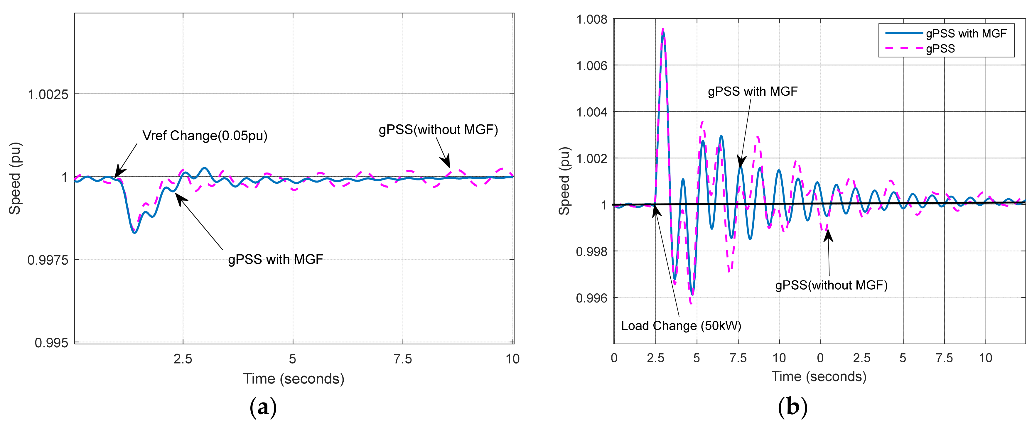
• We propose that adding an MGF to PSS input signals can guarantee the performance of the PSS in microgrids (i.e., systems with changing networks of the power system). The weakness of the PSS is made up for in low-inertia power systems because the perturbation of the power system is considered in the input signal of the PSS by the MGF. SGs operating in microgrids do not have large capacities, but they have a large proportion of relative capacity (e.g., compared to the generation capacity of the entire power system). Therefore, the swing of this SG is closely related to the system frequency variation. In other words, as the perturbation of the SG causes changes in the frequency of the power system, the deviation of speed, the signal used by the gPSS, is valid for large power systems with almost constant frequency of the power system, but not for microgrids. In case study #1, differences depending on whether an MGF is applied or not are clearly identified. In case study #3, the gPSS without an MGF shows that the oscillation does not attenuate but persists until the end of the simulation. The oscillation persists even longer than that without a PSS. These results demonstrate the linkage characteristics of the frequencies between the microgrid and the SG and the validity of the MGF.
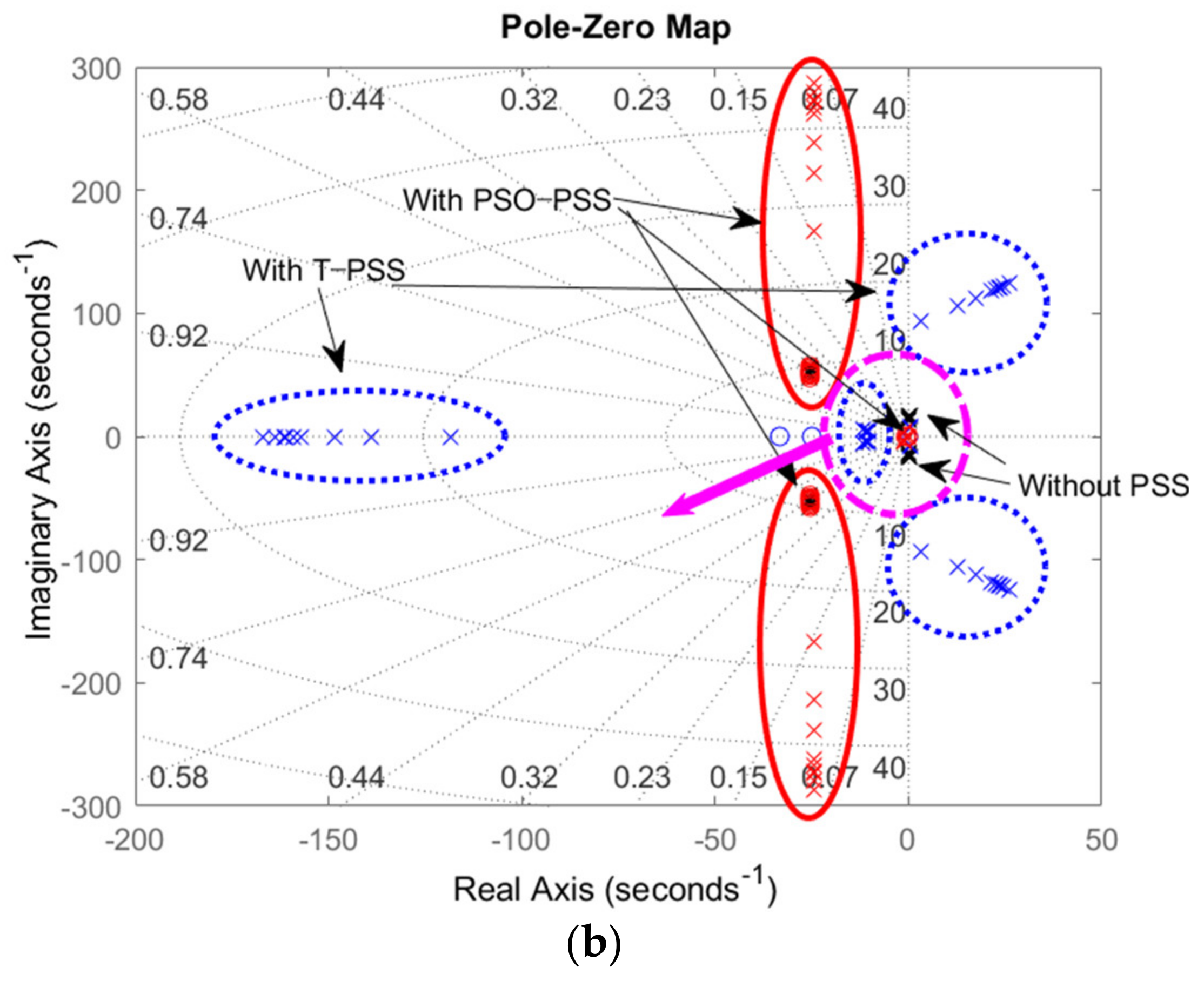
• In LFS mode, the effects on MCs can be seen through frequency characteristic analysis of the linearized models (i.e., GEP and SMNB models). Differences in frequency characteristics of the GEP model by the MC are demonstrated in Figure 9 through the Bode diagram analysis.
• The

  Table 5. Bode diagram analysis with 3 operating points.

  Operating Point	Magnitude of μPSS at 0.025 Hz (Abs)	Magnitude of gPSS at 0.039 Hz (Abs)	Phase of μPSS at 10 Hz (Degree)	Phase of gPSS at 10 Hz (Degree)
  1	8574	5201	−52.29	−54.31
  5	15,136	9176
  9	14,294	8669

  summarizes the main features of the Bode analysis, showing that there is no significant change in the actual phase characteristics (some improvements) but an improvement in the magnitude of the key areas (0.01–10 Hz) that the PSS of the SG should be able to compensate. In other words, comparing the phase and magnitude frequency characteristics of the μPSS with those of the gPSS, it can be determined that in the case where the μPSS is applied, the performance has improved in all areas requiring damping torque supply by the PSS.
• It is confirmed in Figure 9 that the poles of the electro-mechanical mode move further to the left side in the s-plane. In particular, the

  Table 6. Location of the pole in electro-mechanical mode.

  Operating Point	μPSS		gPSS
  	Damping (% Overshoot)	Poles	Damping (% Overshoot)	Poles
  1	0.345 (31.5%)	−1.14 + j3.09	0.259 (43%)	−0.991 + j3.69
  2	0.374 (28.2%)	−1.14 + j2.84	0.283 (39.6%)	−1 + j3.4
  3	0.409 (24.4%)	−1.16 + j2.58	0.313 (35.5%)	−1.02 + j3.1
  4	0.279 (40.1%)	−1.12 + j3.85	0.207 (51.5%)	−0.961 + j455
  5	0.392 (26.2%)	−1.16 − j2.72	0.299 (37.3%)	−1.02 − j3.27
  6	0.403 (25.1%)	−1.15 + j2.62	0.308 (36.2%)	−1.02 + j3.14
  7	0.396 (25.8%)	−1.15 + j2.67	0.302 (36.9%)	−1.02 + j3.2
  8	0.366 (29.9%)	−1.16 + j2.94	0.277 (40.4%)	−1.02 + j3.54
  9	0.387 (26.8%)	−1.16 + j2.76	0.294 (38%)	−1.02 + j3.31
  10	0.413 (24.1%)	−1.15 − j2.54	0.316 (35.1%)	−1.02 + j3.05
  Average	0.3764	-	0.2858	-

  shows an average 31.7% increase in damping torque, thereby mitigating overshooting. The analysis results show that the damping performance for LFOs is enhanced by the novel structures (MC and SIC) that are added to the μPSS proposed in this paper.
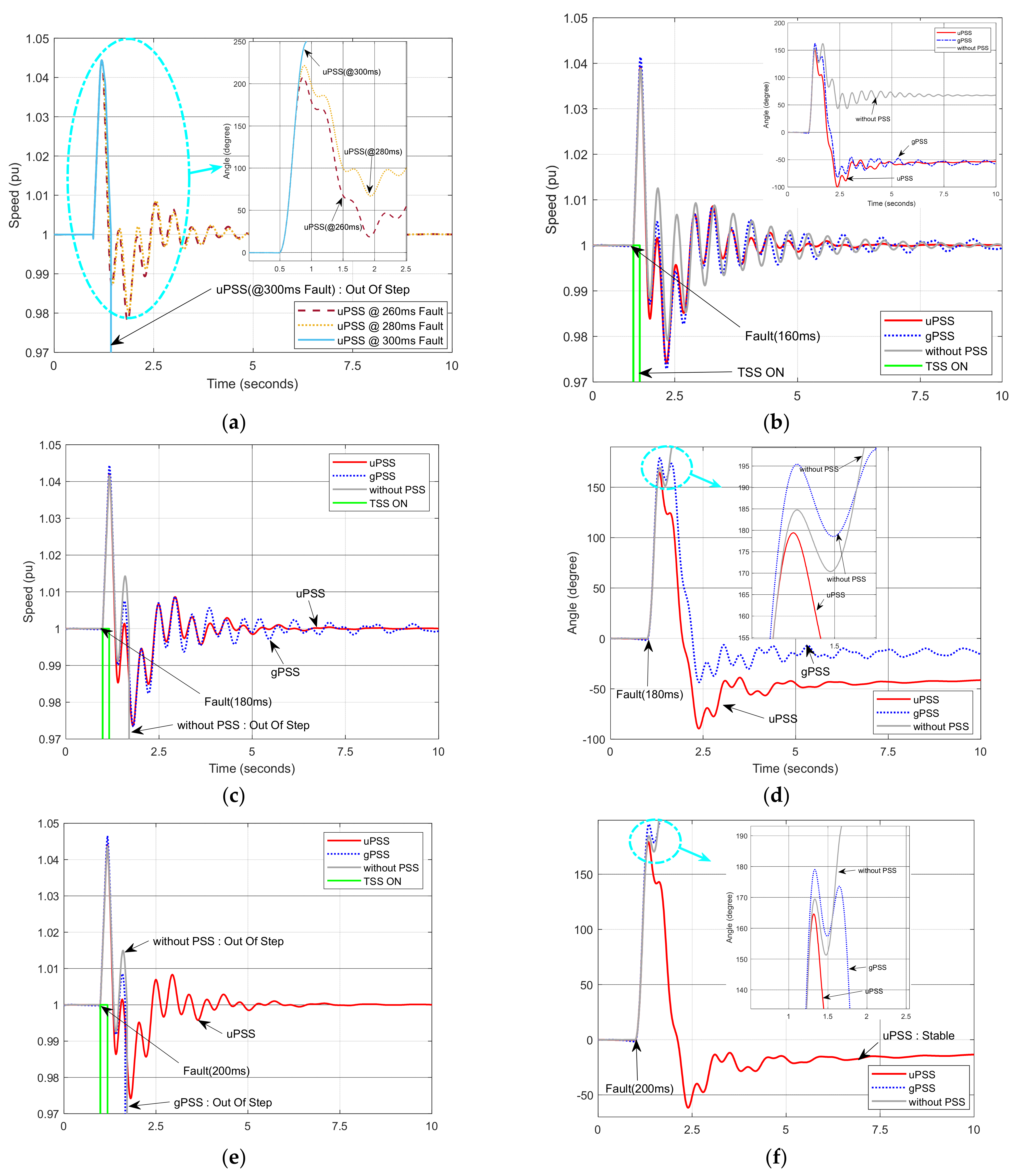
• In TSS mode, the excitation Boosting (EB) control is performed through the Lyapunov energy-function-based control strategy to provide additional synchronizing power during large disturbances. TSS mode helps to maintain continuous synchronization in cases where the microgrids undergo failure or significant load changes (e.g., transition to islanded operation, tripping a part of the system, etc.). The

  Table 7. The effects on the transient stability.

  Criterion *	μPSS	gPSS	Without a PSS	Figure No.
  Critical clearing time	280 ms	180 ms	160 ms	12
  Permissible load change **	700 kW	600 kW	500 kW	13

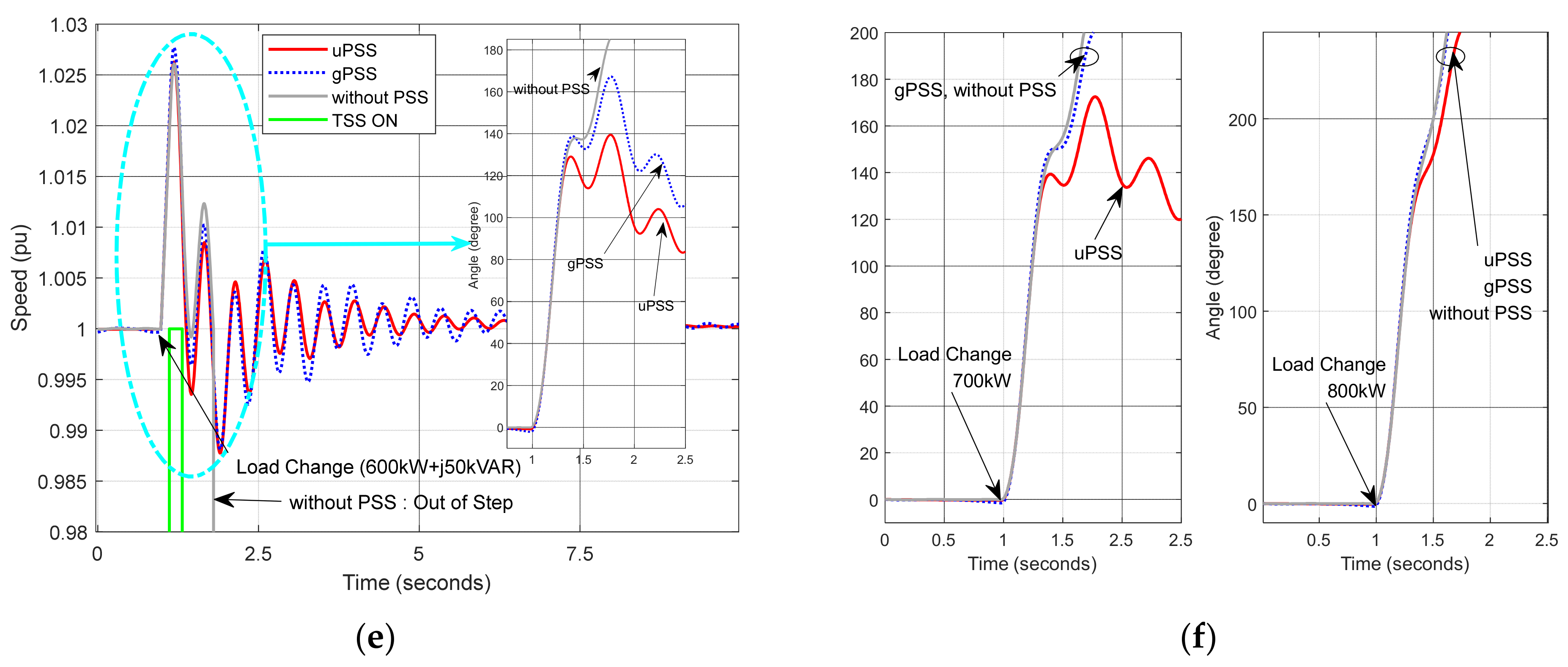
  * These criteria are influenced by initial conditions of TDS; ** instantaneously permissible load change.

  summarizes the results of a case study to check the effectiveness of the TSS, which shows that the CCT is improved and the allowable load change in the microgrid is increased. Simulation results show that the initial deviation of the phase angle caused by sudden load changes is suppressed by the TSS in Figure 13.
• However, even if the initial phase angle deviation is suppressed by the TSS, it will inevitably exceed the permissible limit of the phase angle between the COI and a generator if the load change eventually becomes unaffordable for one SG. Thus, the initial phase angle difference immediately after load change is suppressed, as in Figure 13. Then the phase difference exceeds the permissible limit of the angle difference in the end. However, it can be inferred that if proper load sharing is possible among other power sources that can adjust power output, it will converge to a stable system later by appropriately sharing the load if only the initial phase angle deviation of the disturbance is endured by the TSS in a SG.

Parameters play a very important role in the performance of a PSS, so in this work, we perform parameter setting using an HOA, particle swarm optimization, to minimize the impact of parameters when comparing the μPSS with the gPSS. That is because we want to focus on the characteristics caused solely by structural differences between the μPSS and the gPSS. The parameter values found using PSO are applied identically to the test target PSSs (i.e., μPSS and gPSS) to verify the superiority of the μPSS with frequency-domain analysis and TDS. Therefore, in this paper, the test results have nothing to do with the parameters of the PSS. In addition, the μPSS has the advantage of being able to be applied by the good tuning methods proposed in many studies, as its structure is the most widely used one based on PSS-2B.

The SG is not only at the core of a conventional power system, but it also plays a crucial role in microgrids. The $\mathsf{\mu }$PSS is expected to contribute significantly to stability enhancement of the microgrids.

References

1. Lasseter, R.H.; Paigi, P. Microgrid: A conceptual solution. In Proceedings of the 2004 IEEE 35th Annual Power Electronics Specialists Conference (IEEE Cat. No. 04CH37551), Aachen, Germany, 20–25 June 2004. [Google Scholar]
2. Bhaskara, S.N.; Chowdhury, B.H. Microgrids—A review of modeling, control, protection, simulation and future potential. In Proceedings of the 2012 IEEE Power and Energy Society General Meeting, San Diego, CA, USA, 22–26 July 2012. [Google Scholar]
3. Hirsch, A.; Parag, Y.; Guerrero, J. Microgrids: A review of technologies, key drivers, and outstanding issues. Renew. Sustain. Energy Rev. 2018, 90, 402–411. [Google Scholar] [CrossRef]
4. Farrokhabadi, M.; Cañizares, C.A.; Simpson-Porco, J.W.; Nasr, E.; Fan, L.; Mendoza-Araya, P.A.; Tonkoski, R.; Tamrakar, U.; Hatziargyriou, N.; Lagos, D. Microgrid stability definitions, analysis, and examples. IEEE Trans. Power Syst. 2019, 35, 13–29. [Google Scholar] [CrossRef]
5. San, G.; Zhang, W.; Guo, X.; Hua, C.; Xin, H.; Blaabjerg, F. Large-disturbance stability for power-converter-dominated microgrid: A review. Renew. Sustain. Energy Rev. 2020, 127. [Google Scholar] [CrossRef]
6. Lidula, N.; Rajapakse, A. Microgrids research: A review of experimental microgrids and test systems. Renew. Sustain. Energy Rev. 2011, 15, 186–202. [Google Scholar] [CrossRef]
7. Abido, M. Optimal design of power-system stabilizers using particle swarm optimization. IEEE Trans. Energy Convers. 2002, 17, 406–413. [Google Scholar] [CrossRef]
8. Kundur, P.; Balu, N.J.; Lauby, M.G. Power System Stability and Control; McGraw-Hill: New York, NY, USA, 1994; Volume 7. [Google Scholar]
9. Obaid, Z.A.; Cipcigan, L.; Muhssin, M.T. Power system oscillations and control: Classifications and PSSs’ design methods: A review. Renew. Sustain. Energy Rev. 2017, 79, 839–849. [Google Scholar] [CrossRef]
10. Kamwa, I.; Grondin, R.; Trudel, G. IEEE PSS2B Versus PSS4B: The Limits of Performance of Modern Power System Stabilizers. IEEE Trans. Power Syst. 2005, 20, 903–915. [Google Scholar] [CrossRef]
11. Liu, Z.; Yao, W.; Wen, J. Enhancement of Power System Stability Using a Novel Power System Stabilizer with Large Critical Gain. Energies 2017, 10, 449. [Google Scholar] [CrossRef]
12. Dudgeon, G.J.W.; Leithead, W.E.; Dysko, A.; O’Reilly, J.; McDonald, J.R. The Effective Role of AVR and PSS in Power Systems: Frequency Response Analysis. IEEE Trans. Power Syst. 2007, 22, 1986. [Google Scholar] [CrossRef]
13. Larsen, E.; Swann, D. Applying power system stabilizers part I: General concepts. IEEE Trans. Power Appar. Syst. 1981, 6, 3017–3024. [Google Scholar] [CrossRef]
14. Larsen, E.; Swann, D. Applying power system stabilizers part II: Performance objectives and tuning concepts. IEEE Trans. Power Appar. Syst. 1981, 6, 3025–3033. [Google Scholar] [CrossRef]
15. Larsen, E.; Swann, D. Applying power system stabilizers Part III: Practical considerations. IEEE Trans. Power Appar. Syst. 1981, 6, 3034–3046. [Google Scholar] [CrossRef]
16. Gurrala, G.; Sen, I. Power System Stabilizers Design for Interconnected Power Systems. IEEE Trans. Power Syst. 2010, 25, 1042. [Google Scholar] [CrossRef]
17. Kumar, A. Power System Stabilizers Design for Multimachine Power Systems Using Local Measurements. IEEE Trans. Power Syst. 2016, 31, 2163–2171. [Google Scholar] [CrossRef]
18. Movahedi, A.; Niasar, A.H.; Gharehpetian, G. Designing SSSC 2171, TCSC, and STATCOM controllers using AVURPSO, GSA, and GA for transient stability improvement of a multi-machine power system with PV and wind farms. Int. J. Electr. Power Energy Syst. 2019, 106, 455–466. [Google Scholar] [CrossRef]
19. Panda, S.; Padhy, N.P. Comparison of particle swarm optimization and genetic algorithm for FACTS-based controller design. Appl. Soft Comput. 2008, 8, 1418–1427. [Google Scholar] [CrossRef]
20. Shayeghi, H.; Safari, A.; Shayanfar, H.A. PSS and TCSC damping controller coordinated design using PSO in multi-machine power system. Energy Convers. Manag. 2010, 51, 2930–2937. [Google Scholar] [CrossRef]
21. Verdejo, H.; Pino, V.; Kliemann, W.; Becker, C.; Delpiano, J. Implementation of Particle Swarm Optimization (PSO) Algorithm for Tuning of Power System Stabilizers in Multimachine Electric Power Systems. Energies 2020, 13, 2093. [Google Scholar] [CrossRef] [Green Version]
22. Jolfaei, M.G.; Sharaf, A.M.; Shariatmadar, S.M.; Poudeh, M.B. A hybrid PSS–SSSC GA-stabilization scheme for damping power system small signal oscillations. Int. J. Electr. Power Energy Syst. 2016, 75, 337–344. [Google Scholar] [CrossRef]
23. Rahmatian, M.; Seyedtabaii, S. Multi-machine optimal power system stabilizers design based on system stability and nonlinearity indices using Hyper-Spherical Search method. Int. J. Electr. Power Energy Syst. 2019, 105, 729–740. [Google Scholar] [CrossRef]
24. Aderibole, A.; Zeineldin, H.H.; Al Hosani, M. A Critical Assessment of Oscillatory Modes in Multi-Microgrids Comprising of Synchronous and Inverter-Based Distributed Generation. IEEE Trans. Smart Grid 2019, 10, 3320–3330. [Google Scholar] [CrossRef]
25. Alaboudy, A.K.; Zeineldin, H.H.; Kirtley, J. Microgrid stability characterization subsequent to fault-triggered islanding incidents. IEEE Trans. Power Deliv. 2012, 27, 658–669. [Google Scholar] [CrossRef]
26. Majumder, R. Some aspects of stability in microgrids. IEEE Trans. Power Syst. 2013, 28, 3243–3252. [Google Scholar] [CrossRef]
27. Shuai, Z.; Sun, Y.; Shen, Z.J.; Tian, W.; Tu, C.; Li, Y.; Yin, X. Microgrid stability: Classification and a review. Renew. Sustain. Energy Rev. 2016, 58, 167–179. [Google Scholar] [CrossRef]
28. Bedi, J.; Toshniwal, D. Empirical Mode Decomposition Based Deep Learning for Electricity Demand Forecasting. IEEE Access 2018, 6, 49144–49156. [Google Scholar] [CrossRef]
29. Moradzadeh, A.; Zakeri, S.; Shoaran, M.; Mohammadi-Ivatloo, B.; Mohammadi, F. Short-Term Load Forecasting of Microgrid via Hybrid Support Vector Regression and Long Short-Term Memory Algorithms. Sustainability 2020, 12, 76. [Google Scholar] [CrossRef]
30. Zamee, M.A.; Won, D. Novel Mode Adaptive Artificial Neural Network for Dynamic Learning: Application in Renewable Energy Sources Power Generation Prediction. Energies 2020, 13, 405. [Google Scholar] [CrossRef]
31. Ceci, M.; Corizzo, R.; Malerba, D.; Rashkovska, A. Spatial autocorrelation and entropy for renewable energy forecasting. Data Min. Knowl. Discov. 2019, 33, 698–729. [Google Scholar] [CrossRef]
32. Cavalcante, L.; Bessa, R.J.; Reis, M.; Browell, J. LASSO vector autoregression structures for very short-term wind power forecasting. Wind Energy 2017, 20, 657–675. [Google Scholar] [CrossRef] [Green Version]
33. Rahman Fahim, S.K.; Sarker, S.; Muyeen, S.M.; Sheikh, M.R.I.; Das, S.K. Microgrid Fault Detection and Classification: Machine Learning Based Approach, Comparison, and Reviews. Energies 2020, 13, 3460. [Google Scholar] [CrossRef]
34. Cepeda, C.; Orozco-Henao, C.; Percybrooks, W.; Pulgarín-Rivera, J.D.; Montoya, O.D.; Gil-González, W.; Vélez, J.C. Intelligent Fault Detection System for Microgrids. Energies 2020, 13, 1223. [Google Scholar] [CrossRef] [Green Version]
35. Hosseinzadeh, M.; Rajaei Salmasi, F. Islanding Fault Detection in Microgrids—A Survey. Energies 2020, 13, 3479. [Google Scholar] [CrossRef]
36. Li, L.; Li, H.; Tseng, M.-L.; Feng, H.; Chiu, A.S.F. Renewable Energy System on Frequency Stability Control Strategy Using Virtual Synchronous Generator. Symmetry 2020, 12, 1697. [Google Scholar] [CrossRef]
37. Pinthurat, W.; Hredzak, B. Decentralized Frequency Control of Battery Energy Storage Systems Distributed in Isolated Microgrid. Energies 2020, 13, 3026. [Google Scholar] [CrossRef]
38. SPilehvar, M.; Mirafzal, B. Frequency and Voltage Supports by Battery-Fed Smart Inverters in Mixed-Inertia Microgrids. Electronics 2020, 9, 1755. [Google Scholar] [CrossRef]
39. Baneshi, E.; Kolahduzloo, H.; Ebrahimi, J.; Mahmoudian, M.; Pouresmaeil, E.; Rodrigues, E.M.G. Coordinated Power Sharing in Islanding Microgrids for Parallel Distributed Generations. Electronics 2020, 9, 1927. [Google Scholar] [CrossRef]
40. Cheng, H.; Shuai, Z.; Shen, C.; Liu, X.; Li, Z.; Shen, Z.J. Transient Angle Stability of Paralleled Synchronous and Virtual Synchronous Generators in Islanded Microgrids. IEEE Trans. Power Electron. 2020, 35, 8751–8765. [Google Scholar] [CrossRef]
41. Sauer, P.W.; Pai, M.A. Power System Dynamics and Stability; Wiley Online Library: Hoboken, NJ, USA, 1998; Volume 101. [Google Scholar]
42. Ahmadi, H.; Kazemi, A. The Lyapunov-based stability analysis of reduced order micro-grid via uncertain LMI condition. Int. J. Electr. Power Energy Syst. 2020, 117. [Google Scholar] [CrossRef]
43. Veerashekar, K.; Schuehlein, P.; Luther, M. Quantitative transient stability assessment in microgrids combining both time-domain simulations and energy function analysis. Int. J. Electr. Power Energy Syst. 2020, 115. [Google Scholar] [CrossRef]
44. Pai, M. Energy Function Analysis for Power System Stability; Springer Science & Business Media: Berlin, Germany, 2012. [Google Scholar]
45. Machowski, J.; Robak, S.; Bialek, J.; Bumby, J.; Abi-Samra, N. Decentralized stability-enhancing control of synchronous generator. IEEE Trans. Power Syst. 2000, 15, 1336–1344. [Google Scholar] [CrossRef]
46. Diez-Maroto, L.; Renedo, J.; Rouco, L.; Fernandez-Bernal, F. Lyapunov Stability Based Wide Area Control Systems for Excitation Boosters in Synchronous Generators. IEEE Trans. Power Syst. 2019, 34, 194–204. [Google Scholar] [CrossRef]
47. IEEE Standard 421.5-2016. IEEE Recommended Practice for Excitation System Models for Power System Stability Studies; IEEE: New York, NY, USA, 2016. [Google Scholar] [CrossRef]
48. Zhang, T.; Mao, C.; Zhang, J.; Tian, J.; Yu, M.; Wu, K.; Xiong, H.; Wu, L.; Yu, H. Design and Field Application of Flexible Excitation System Damping Controllers. IEEE Trans. Ind. Electron. 2021, 68, 949–959. [Google Scholar] [CrossRef]
49. Gibbard, M.; Vowles, D. Design of power system stabilizers for a multi-generator power station. In Proceedings of the PowerCon 2000 International Conference on Power System Technology. Proceedings (Cat. No. 00EX409), Perth, WA, Australia, 4–7 December 2000. [Google Scholar]
50. Gibbard, M.J.; Vowles, D.J. Reconciliation of methods of compensation for PSSs in multimachine systems. IEEE Trans. Power Syst. 2004, 19, 463–472. [Google Scholar] [CrossRef]
Figure 1. Single-machine infinite bus (SMIB) model.
Energies 14 00905 g001
Figure 2. Variation of the magnitude of synchronous impedance.
Energies 14 00905 g002
Figure 3. Single-machine microgrid system.
Energies 14 00905 g003
Figure 4. The micro-power system stabilizer ( μ PSS): (a) overall structure of the μPSS and (b) the functional features of the μPSS.
Energies 14 00905 g004
Figure 5. The D-shaped sector in the negative half of the s-plane.
Energies 14 00905 g005
Figure 6. Linearized model of a single machine connected to a non-stiff bus.
Energies 14 00905 g006
Figure 7. PSS parameter tuning by particle swarm optimization: (a) objective function optimization flowchart and (b) particle swarm optimization results for PSS parameter tuning.
Energies 14 00905 g007aEnergies 14 00905 g007b
Figure 8. Stability analysis of and single-machine non-stiff bus (SMNB) model depending on the parameter of PSS-2B (red solid line is the PSS tuned by PSO, blue dashed line is the PSS with typical parameters, black dotted line is the case without a PSS): (a) Bode diagram of the generator-exciter-PSS (GEP) model and (b) pole location of the SMNB model.
Energies 14 00905 g008aEnergies 14 00905 g008b
Figure 9. μ PSS stability analysis by frequency-domain characteristic of the GEP and SMNB models (solid line: with μ PSS; dashed line: with gPSS): (a) Bode diagram of the GEP model with 3 operating points, (b) pole zero map of the SMNB model with 10 operating points, and (c) pole location of the electro-mechanical mode of the SMNB model with 10 operating points.
Energies 14 00905 g009
Figure 10. Step response in the SMNB model: (a) step size 0.3 in operating point #1, (b) step size 0.3 in operating point #3, (c) step size 0.3 in operating point #5, (d) step size 0.3 in operating point #7, (e) step size 0.6 in operating point #1, (f) step size 0.6 in operating point #3, (g) step size 0.6 in operating point #5, and (h) step size 0.6 in operating point #7.
Energies 14 00905 g010aEnergies 14 00905 g010b
Figure 11. Generator speed variations with small disturbances (system load: 3 MW; initial loading of SG: 0.5 pu (1 MW); reference voltage of AVR: 1 pu): (a) In the case of the reference voltage change (0.05 pu) and (b) In the case of the load change (50 kW).
Energies 14 00905 g011
Figure 12. The effects of the μPSS on transient stability in the case of the three-phase short-circuit fault (fault resistance 0.001 Ω; the fault location is marked with X in Figure A1): (a) critical clearing time of the μPSS (dashed line: 260 ms; dotted line: 280 ms; solid line: 300 ms). (b) In the case of 160 ms three-phase short-circuit fault ( μ PSS: stable; others: unstable (out of step)). (c,d) In the case of 180 ms three-phase short-circuit fault (the case without a PSS: out of step), the trend of speed and phase angle. (e,f) In the case of 200 ms three-phase short-circuit fault with transient state stabilizing (TSS) signals, the trend of speed (only the μPSS case is stable).
Energies 14 00905 g012
Figure 13. Performances of low-frequency stabilizing (LFS) and TSS at the load change (system load: 3 MW; initial loading of SG: 0.5 pu (1 MW); reference voltage of AVR: 1 pu): (a,b) in the case of 300 kW load change, (c,d) in the case of 500 kW load change, (e) in the case of 600 kW load change, and (f) in the case of 700 kW and 800 kW load change (every case is unstable at 800 kW load change).
Energies 14 00905 g013aEnergies 14 00905 g013b