Abstract
Energy power flows are an important factor to be calculated and, thus, are needed to be enhanced in an electrical generation system. It is very necessary to optimally locate the Flexible Alternating Current Transmission Systems (FACTS) devices and improve the Available Transfer Capability (ATC) of the power transmission lines. It relieves the congestion of the system and increases the flow of power. This research study has been accomplished in two stages: optimization of location of FACTS device by the novel Sensitivity and Power loss-based Congestion Reduction (SPCR) method and the calculation of ATC using the proposed Metaheuristic Evolutionary Particle Swarm Optimization (MEEPSO) technique. The Thyristor Controlled Series Capacitor (TCSC) is used as a FACTS device to control the reactance of power transmission line. The effectiveness of the proposed methods is validated, utilizing the six bus as well as 30 bus system. The acquired outcomes are contrasted with conventional ACPTDF and DCPTDF procedures. These values are determined with the assistance of MATLAB version 2017 on the Intel Core i5 framework by taking two-sided exchanges and they are contrasted and values determined with the assistance of Power World Simulator (PWS) programming.
1. Introduction
The power system has gone through a significant change in the most recent many years. Previously, the electric industry has been either an administration controlled or an administration directed industry, which existed as a syndication in its administration area. The huge element of these progressions is to take rivalry among generators of power into account and to make an economic situation in the business, which are viewed as important in expanding the proficiency of electric energy creation and appropriation, and to offer lower costs, higher caliber, and safer item. In the monopolistic structure, the generation, transmission, distribution, and control in a region are overseen by one organization or office that offered electric force and offered types of assistance to all clients, for example, the power is considered as an energy flexible area. While, in the emerging restructured competitive market, the different undertakings are isolated and they must be independently paid by the executing parties, for example, the power is treated as an assistance area and it is to be advertised as another normal ware. The transmission of power itself can be treated as a particular assistance. There are qualifications in the deregulated structure and, along these lines, there exist various game plans of open access to transmission frameworks. All things considered, each restructuring plan must address the crucial specialized issues that are related with the safe and solid activity of the transmission organization.
1.1. General
A significant increase in power transfers involves non-discriminatory open access to transmission networks and it has resulted in a range of technological challenges, including the evaluation of the optimal Available Transfer Capabilities (ATC), to ensure safe transactions.
The ATC indicates the power system’s ability to efficiently increase the transferred power for commercial trading between two zones or two points. The conservative ATC estimate may result in inefficient use of the transmission network. Accordingly, it has to be rapidly and accurately calculated. The ATC value will direct the business behavior of the participants in electricity markets with open access transmission and then develop the transmission capacity to be used proficiently.
The assets must be pooled intensively for the tractability, steadfastness, and frugality of the interconnected power networks. More than one line can be encumbered in the transmission network during open access and, hence, causes congestion. The management of congestion can be effectively achieved by convalescing ATC of the network. In addition, mounting FACTS will increase the deployment of available system capabilities. The FACTS is the use of devices for power electronics to control line flows. Even though the FACTS arrangement involves hefty capital cost, the power system can be wrought in an additional optimized manner, leading to enormous savings. The placement of such devices can be an encouraging strategy to drop congestion of the transmission lines and to escalate ATC. Consequently, there is an interest in learning the stimulus of these devices on ATC plus optimally locating them to augment the transfer capabilities.
The transfer capability is the degree of the aptitude of organized electric networks to change or transfer power efficiently from one region to another under defined system conditions. The transmission transfer limits that are calculated to sustain the consistency of the interrelated transmission networks are called “capabilities”. These limits vary from “capacities”, because they are highly dependent on the conditions of the generation, customer demand, and transmission system that are assumed to be analyzed during the time, while “capacities” are usually used as a specific limit or equipment level, such as the thermal limit or the rating of a specific transmission element or part. Figure 1 depicts the ATC and related terms, which are forming the basis to schedule transmission services in the open power market. These are briefed as:
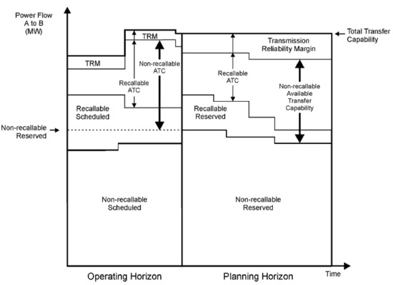
Figure 1.
Various terms for scheduling the transmission service.
The Available Transfer Capability (ATC) is the amount of transfer aptitude that lasts for the additional commercial operation over and beyond previously committed uses of the physical transmission network. This can be deduced by subtracting Transmission Reliability Margin (TRM), Capacity Benefit Margin (CBM), and current power flow from Total Transfer Capability (TTC). The ETC is the sum of the current commitment to transmission between those regions.
Total Transfer Capability (TTC) is the amount of transferable electric power over the interconnected transmission network reliably satisfying pre- and post-contingency system conditions. The TTC refers to the maximum transferable power from one area of power control to the others that do not cause thermal overloads, voltage limit destructions, voltage collapse, or any of the other system complications. Transmission Reliability Margin (TRM) is the transfer capability that is necessary to for ensuring the interconnected transmission in order to secure under a realistic range of uncertainties in the system conditions. It accounts for the intrinsic ambiguity in the transmission system.
The Capacity Benefit Margin (CBM) is the quantity of transmission transfer capability that is reserved by load-serving entities to ensure access to generation from interconnected systems in order to fulfil the requirements of generation reliability. The CBM accounts for uncertainty in the generation. Curtailability refers to the transmission provider’s right to completely or partially interrupt the transmission service due to limitations that decrease the capability of the transmission network, i.e., the cases where the reliability of the system is endangered or emergency conditions exist. Recallability refers to the service provider’s right to interrupt all or part of transmission service because of any reason, including economic, which adheres to the FERC policy and provisions of the contract.
Non-recallable ATC (NATC) may be stated as TTC, excluding TRM and non-recallable reserved transmission service. Recallable ATC (RATC) is expressed as TTC, excluding TRM, recallable transmission service, and non-recallable transmission service (including CBM). The control free power system is a larger area, and the literature explains different operation and control aspects. Power market participants and competitive environment are provided by the open-access transmission network which is due to the deregulation. The FACTS devices are capable of changing the parameters of a system efficiently and quickly, and it can suitably control the flow of power.
In the era of restructured power system, the independent system operator (ISO) is responsible for controlling the power transactions and preventing the overloading of the transmission lines beyond the permissible value of thermal loading in Mega Volt-Ampere (MVA). The available transfer capability (ATC) needs to be updated by ISO to achieve this. Therefore, a faster estimation is needed to estimate it quickly in order to provide the real-time requirements apart from preserving the correctness to the desired level. The brief review complements the work that was done by different researchers and identifies the further scope.
1.2. Literature Survey
The transfer capability refers to the unutilized transfer capability of a transmitting network that is available for transactions to the participants in the market. Its accurate and fast estimation, including margins of transmission, remains the key factor in congestion management and its planning [1].
Because power transmission amenities have some physical constraints, entire power transactions cannot be acknowledged. Further, the expansion of new generation and transmission facilities become hindered due to ecological constraints and economic contemplations. Various methods have been reported earlier to estimate ATC based on conventional power system equations. The methods that are based on DC load flow [2] involve less computation complexity and are faster. The methods assume the network to be loss-free and can only model real power flow (in MW). Moreover, voltage limits without being taken care of are incompetent to deliver precise estimation when MVA flows are considered.
The Continuation Power Flow methods (CPF) and Repeated Power Flows (RPF) repeat a full-scale AC load flow solution per increment (over the basic case value) of the load at the sink until any line in the system becomes over-loaded. In these methods, the impact of voltage and reactive power has been accounted for. Although accurate computation complexity is more while being implemented on a large system, and the optimal generation is ignored. The methods that are based on optimal power flow (OPF) provide the optimal settings of controllable variables by optimizing the objective function subjected to equality and inequality constraints. The methods that are based on distribution factors [3] can accommodate the scenarios that are near to the base case. For this purpose, the factors based on power transfer/outage are derived. The linear ATC method [4] that is based on linear distribution factors provides the approximate ATC value. The methods using sensitivity indices [5] can quickly calculate ATC. However, accuracy cannot be maintained when there are significant changes in the system. ATC can be estimated based on probabilistic methods [6]. The probabilistic methods are suited for offline planning analysis.
The FACTS devices offer an active source of power transfer capacity enhancement and they can also be used for the enhancement of transfer capability [7]. Although, the degree to which ATC can be enhanced by FACTS controller is dependent on its optimum position in the system. The various FACTS controllers, namely TCSC (Thyristor Controlled Series Compensator), SVC (Static Var Compensators), STATCOM (Static Synchronous Compensators), and UPFC (Unified Power Flow Controller), have been used for the purpose in [8].
The TCSC offers a series compensation and comprises of a series capacitor bank shunted by Thyristor Controlled Reactor (TCR). With the thyristors control, TCR is capable of changing its reactance smoothly and quickly. TCSC’s static model is used in [9], as a series reactance with the control parameter . Ghawghawe and Thakre [10] suggested a criterion for determining the change in the reactance of TCSC, being necessary for achieving the chosen transfer capability. The changes in the line flow and selection of a line for the installation of TCSC is computed by the sensitivity analysis. Rashidinejad et al. [11] presented a method for determining the optimal location and capacity of TCSC to surge ATC along with the voltage profile. Gaur et al. [12] listed a procedure to recognize the optimum location of FACTS controllers for TTC enhancement. Network strengthening has been given by Huang et al. [13] with the aim of enhancing the ATC of an unified power system with TCSC. Pankajam et al. [14] analyzed the viability and technical merits of boosting ATC while using TCSC.
The shunt controllers, namely SVC and STATCOM, the Unified Power Flow Controller (UPFC), have the capability of active power flow control and they also been investigated for ATC improvement plus the application of SVC and TCSC in TTC improvement, while taking static security limits into consideration [15]. Ibraheem et.al [16] deduced a procedure, on the basis of stochastic programming, in order to improve ATC at the prescribed interface using UPFC. Schnurr et al. [17] deliberated a sensitivity-based method to optimize the location of multifunctional FACTS instruments and their capacity in ATC development. Gupta et al. discussed the application of UPFC for the enhancement of static ATC [18]. Alam et al. [19] presented an improvement in transient stability, using different FACTS controllers having various control strategies. Nireekshana et al. [20] applied FACTS devices for the improvement of voltage profile along with maximum ATC bearing in mind low prices.
Various Artificial Intelligence (AI) techniques, which are emulating one or the other life characteristic, have been evolved, due to the research on artificial life. Among these techniques based on Artificial Neural Network (ANN), Fuzzy Logic, and Evolutionary search algorithms are very popular and they are extensively used in the power system. These techniques have also been used for the computation of transfer capability or the allocation of FACTS devices.
Artificial Neural Networks (ANNs) possess the capability to produce compound mappings precisely and quickly. Because of the toughness, speed, and capacity to handle imperfect or noisy data, the ANNs have been used to estimate transfer capability [21,22,23]. Moreover, the RBFNN can augment new training data without the need for retraining. The static ATC using the RBFNN-based method has been determined in electric markets, with bilateral and multilateral transactions. With the ability to adapt the wavelet shape, as per the training data set and the higher rates of convergence, the wavelet neural networks (WNNs) have shown their excellent performance in non-linear function modeling [24,25,26].
Fuzzy-based approaches deal with uncertainties that are always existing in power system planning [27]. Fuzzy logic can solve non-linear problems at ease and it involves less computation complexity [28,29]. The use of fuzzy logic for OPF has been discussed in [30,31], whereas the fuzzy logic for ATC calculation was discussed by Ahmed et al. [32,33]. The Sugeno fuzzy model was used with three variables, namely sink busload, adjoining bus injection, and a suitably defined loading-index to calculate ATC. With the small set of input variables, the method can be applied for a large-scale power network. In order to determine ATC during uncertainty, an algorithm of fuzzy set theory to CPF is presented by Kim et.al. It can control concurrent doubts in the load limits and bus injections. The major ambiguity factors that affect the ATC are regarded as fuzzy parameters that are conditional on their feasibility distributions. The fuzzy logic is used in contingency constrained OPF [34] to calculate the ATC. The minimization of both pre contingency operating costs and the post contingency correction is attempted.
For the complicated nonlinear and non-differentiable objective functions, the population-based heuristic search and optimization methods, for instance, Genetic Algorithm (GA), Evolutionary Programming (EP), Particle Swarm Optimization (PSO), etc. search using a population of solution optimally in the feasible domain. The GA and EP are the evolutionary algorithms that are natural selection and survival of fittest based. These algorithms emphasize the behavioral linkage between parents and their off-springs to search for an optimal solution. The PSO is based on the social behavior metaphor and it has fast convergence.
These evolutionary algorithms have been applied for optimum power flow solutions [35,36,37,38,39,40,41] forming a bidding strategy [42,43,44] under the deregulated environment and transfer capacity evaluation. Othman et al. [45] described the application of evolutionary algorithms in determining the capacity benefit margin (CBM) in a power system. The CBM has been calculated by maximizing the total generation capacity. The EP performance is enhanced by means of the improved Gaussian formulation for generating offspring.
The PSO is also used for various power system optimization purposes. Few of these applications include the evaluation of optimal power flow [46], transient stability constrained OPF [47], security-constrained OPF [48], reactive power dispatch [49], and generator scheduling for congestion management. Kennedy [50] analyzed a particle’s trajectory and generated a generalized model of the algorithm which consisted coefficients to control the convergence tendencies of the system and suggested the methods for varying the original algorithm.
Farahmand et al. [51] applied the Genetic Algorithm (GA) with the analytic hierarchy process and fuzzy sets in the form of a hybrid experimental technique to improve the location and capability of TCSC in order to improve ATC along with the voltage profile. Karthiga et al. [52] analyzed the feasibility and technical benefits of furthering ATC by Thyristor Controlled Series Compensator (TCSC) and the PSO algorithm has been applied to optimize the settings of TCSC. Farahmand et al. [53] applied the Real Genetic Algorithm (RGA) linked with Analytical Hierarchy Process (AHP) and fuzzy sets in the form of a hybrid experimental technique for optimizing location and capability of TCSC in order to improve the ATC in addition to voltage profile.
1.3. Gaps in the Research
The following paucities apropos optimal location of FACTS devices and enhancement and comparison of ATC procedure have been recognized from erstwhile work and they are emphasized in this article:
- There is a lack of methods that can imbibe the quality of sensitivity factors and, at the same time, prove that the reactive power losses are reduced and congestion is minimized by reduction of real power [11,54,55].
- There is also dearth of approaches considering optimization of positioning of FACTS device and, hence, increase of ATC [1,3,5,7,8,9,10,12,13,15].
- There is an absence of a comparison of intelligent techniques with the conventional methods and power world simulator results. Additionally, there is very least literature available on the use of Power World Simulator, an upcoming power system software, like MATLAB [2,9,28,29,30,31,32,33,34,35,36,37,39,40,41,42,43,44,46,51,52,53,56,57].
1.4. Contributions
As per the identified gaps, the core methodological contributions of this study are:
- The placement and location optimization of FACTS device to increase the ATC. An innovative method of determining the optimum location of FACTS devices while using the Sensitivity and Power loss-based Congestion Reduction (SPCR) method has been put forward. The Sensitivity and Power loss-based Congestion Reduction (SPCR) method proposes a technique of finding the optimal location of FACTS devices by adopting the technique of first calculating the sensitivity of all the lines in the considered system and then observing the reduction of reactive and real power losses in the most sensitive lines. The lines having reduced losses are verified again by observing the reduction in real power flows. Because the reduction in power flow by placing FACTS devices in these lines will ensure the increase of ATC in these lines and, hence, there will be less congestion in the system. For this, the two factors viz., DC power flow sensitivity factor, and Reactive Power loss reduction factor is calculated when considering contingencies.
- The calculation of enhanced ATC. A new technique for optimizing the value of ATC is proposed, namely MEEPSO (Metaheuristic Evolutionary Particle Swarm Optimization). It is a metaheuristic technique, as it makes not many or no suppositions about the issue being streamlined and it can look through enormous spaces of up-and-comer arrangements. Additionally, MEEPPSO does not utilize the inclination of the issue being advanced, which implies that it does not necessitate that the improvement issue is differentiable, as is required by exemplary streamlining techniques. MEEPSO technique is used, which gives a higher rate of convergence and helps in optimizing the value of ATC. The acceleration parameters c1 and c2 are elected, both equal to value 2 and inertia weights, is fixed at 1, is at 1.2, compensation is sustained at 50%. The number of iterations is 200 and the number of particles is 50. The calculations are executed beneath MATLAB 2017b milieu.
- Power World Simulator software is used for reckoning ATC besides the results are compared with conventional techniques employing MATLAB software. MATLAB software is a very well-established software, but, with time, pristine software should be advanced. The authors have exploited the Simulator GOS Education 21 version of Power World Simulator software to validate and authenticate the results achieved from MATLAB.
1.5. Organization of Paper
In this paper, ATC is calculated while using the proposed MEEPSO technique and the FACTS devices are optimally located with the help of the novel SPCR technique. The attained consequences are judged alongside the outcomes of ACPTDF, DCPTDF techniques in addition to Power World simulator results. The proposed results are relatively advanced in terms of maximizing ATC and ominously minimizing congestion and noteworthy decline in real power flow coupled with diminution in real and reactive power losses and, hence, augmenting the ATC values. The results are assessed for six bus and 30 bus systems. The organization of the paper is as follows: Section 2 defines the Problem and Modeling used. This section covers the importance of ATC, ATC determination using Linear Sensitivity Factors, an algorithm for the calculation of ATC using ACPTDF, the use of Flexible Alternating Current Transmission Systems (FACTS), Thyristor Controlled Series Compensator (TCSC) explanation, the proposed SPCR method for optimally locating FACTS devices, the building of algorithm and parameter choice of MEEPSO technique, and then Power World Simulator is explained. In Section 3, the results are discussed and, finally, in Section 4 and Section 5, the Conclusion and Future scope are presented.
2. Definition of Problem and Modeling
The problem is defined as calculating the available transfer capability in the system by using the ACPTDF technique. The values are improved by optimally placing FACTS devices with the help of the proposed SPCR method in collaboration with the novel MEEPSO algorithm. The results are calculated for six bus and 30 bus systems. Firstly, the importance of ATC is defined in the following section.
2.1. Importance of Available Transfer Capability
The need for using Available Transfer Capability (ATC) [58] arises because of the importance of most reliably delivering the power and also to give flexibility to change the system as and when required. It is also of importance, so that the urge to enhancing more installed generating capacity can be reduced. Mathematically, ATC gives the transfer capability left in the physical transmission network for more commercial activity other than the existing one. It is explained through the following equation:
Where, TTC is Total Transfer Capability, TRM is Transfer Reliability Margin, ETC is Existing Transmission Commitments, and CBM is Capacity Benefit Margin.
2.2. ATC Determination Using Linear Sensitivity Factors
The linear sensitivity elements have a potential for instantaneous calculation of ATC. The use of these parameters provides an estimate, however, extraordinarily fast version for the determination of static ATC. A fresh set of ac power transfer distribution factors (ACPTDFs) for the determination of static ATC greater precisely is proposed in [1]. The coefficient of the linear relation between the transaction amount and drift on a line is termed Power Transfer Distribution Factor (PTDF). PTDFs decide the linear effect of a transfer at the elements of the energy system. These values offer a linear approximation of flow at the transmission lines and interfaces and also observe the change in response to the transaction between the seller and the buyer.
It is based on the Newton Raphson load flow approach. In the AC method, change occurs during line flow sensitivity factors. The calculation of line flows in the ac method is given as:
Using the equation for the N-R Jacobian method:
where is complex power flowing between bus i and j, is and is , is the voltage at the bus, is the current flowing between buses i and j. is the change in real power and is the incremental change in real power regarding the change in angle.
2.3. Algorithm for Calculation of ATC Using ACPTDF
The ac power transfer distribution parameters for calculating ATC are used to determine different transmission system quantities for a variation in MW transaction at variable operating conditions. For instance, abilateral transaction between a seller m and a buyer bus n.The algorithm for the calculation of ATC using ACPTDF is presented below. The equations used in the process are described in the algorithm step-by-step.
- Step 1: Calculate the line flow sensitivity factors
- Step 2: Consider an n-node system having as PV buses and as PQ buses.
- Step 3: Bus 1 is the slack bus. Change in flow for an arbitrary line can be evaluated by sensitivity analysis, as follows:
- Step 4: Transacted Power is between bus to bus :
- Step 5: By the N-R Load Flow:
- Step 6: ATC can be calculated, as given below:
2.4. Use of Flexible Alternating Current Transmission Systems (FACTS)
The FACTS devices refer to power electronics-based devices that are capable of enhancing the controllability and stability of the AC system and, hence, the capability of transferring power is enhanced. Figure 2 shows the model of a transmission line with the FACTS device. Transmission capacity can be enhanced by installing the FACTS device. These devices require less maintenance and they do not experience much wear and tear. But there are some limitations of cost and they are more complex in nature. The noteworthy device from the assembly of FACTS is a TCSC, which finds use in resolving many problems in the power system. Its properties can upsurge the transmission capacity of power lines and control of power flow. It also makes available a varied range of supplementary uses to safeguard the effective, uncomplicated, and cost-effective operation of power systems. It is used to increase the capability of the transfer of power. TCSC finds application in high power and power electronics of high efficiency. The FACTS device is preferred to capacitors switched by circuit breakers, because these are more flexible and advanced. The main controlling factor is XT. The range of XT is taken from 0 to 0.5 XT.
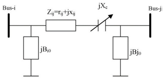
Figure 2.
Model of Transmission line with Flexible Alternating Current Transmission Systems (FACTS) devices.
2.5. Thyristor Controlled Series Compensator (TCSC)
The elementary Thyristor Controlled Series Compensator arrangement was suggested in 1986 as a technique of “quick tuning of network impedance”. The TCSC can be described as a capacitive reactance compensator that contains a series capacitor bank shunted by a thyristor-controlled reactor to deliver a smooth adjustable series capacitive reactance. For realistic TCSC applications, numerous such elementary compensators might be coupled in series to obtain the preferred voltage rating besides operating characteristics. Although, the fundamental notion after the TCSC structure is to make available an incessantly variable capacitor while using partly annulling the actual reimbursing capacitance by the TCR. The vital theoretical TCSC module includes a series capacitor, C, in parallel with a thyristor-controlled reactor. Figure 3 shows the basic module of TCSC.
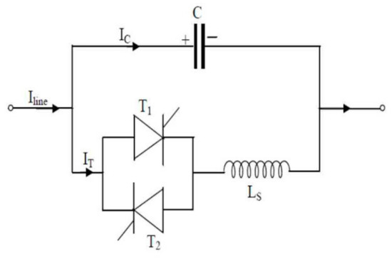
Figure 3.
The basic module of Thyristor Controlled Series Compensator (TCSC).
2.6. Optimal Location of FACTS Device Using Sensitivity and Power Loss Based Congestion Reduction (SPCR) Method
The Sensitivity and Power loss-based Congestion reduction (SPCR) method presents the method of finding the optimal location of FACTS devices by adopting the technique of first calculating the sensitivity of all the lines in the considered system and then observing the reduction of reactive and real power losses in the most sensitive lines. The lines having reduced losses are again verified by observing the reduction in real power flow. Because the reduction in power flow by placing FACTS devices in these lines will ensure the increase of ATC in these lines and, hence, there will be less congestion in the system. Figure 4 shows the flowchart of the recommended SPCR method.
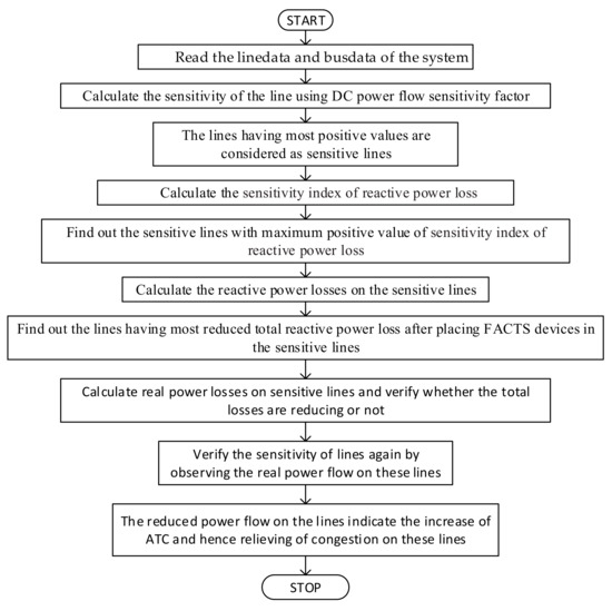
Figure 4.
The flow chart of the proposed Sensitivity and Power Loss Based Congestion Reduction (SPCR) method.
The methods that are adopted for the Optimal Location of FACTS device are first the DC power flow sensitivity factor method and second the Reactive Power loss reduction method. These approaches are described below:
2.6.1. DC Power Flow Sensitivity Factor Method
In the DC power flow sensitivity factor method, the optimal location of TCSC is completed by espousing the procedure that deals with observing sensitivity of real power flow. The parameter
gives the DC power flow sensitivity factor. It gives the loss sensitivity concerning the control parameter
. The DC power flow sensitivity factor is defined by the following equation:
where q, r, and d are the line outage sensitivity factors.
is the change in real power flow on line q and
is the original power flow on line before its outage. In this method, the sensitivity matrix
is calculated while using the dc load flow equation
The DC power flow sensitivity factor is calculated with the help of following equation:
where r efers to the line that is at fault and it is linked amongst buses o and p,
refers to the reactance of the line at which TCSC is to be placed amongst buses s and t. Greater sensitivity factors point toward greater reliance.
2.6.2. Reactive Power Loss Reduction Method
In this method, the optimal location of TCSC is done by adopting the methodology that is grounded on finding the sensitivity of total reactive power loss. The parameter
gives the reactive power loss sensitivity index. It gives the loss sensitivity concerning the control parameter
. The following equation provides the reactive power loss sensitivity index:
where
is the series reactance of the line with FACTS device located amidst i and j buses. Here, the reactance of the FACTS device and resistance of the line is assumed to be negligible.
2.6.3. Criteria for Finding the Location of TCSC:
The FACTS device must be located on the most sensitive line. The sensitivity indices are calculated, and the measures used for its optimal placement can be defined as:
- (a)
- Firstly, for the DC power flow sensitivity factor method, the TCSC device should be located on a line comprising the highest positive DC power flow sensitivity factor, .
- (b)
- Secondly, for the reactive power loss reduction method, the TCSC device should be located on a line that comprises the highest positive reactive power loss sensitivity index, .
2.7. Metaheuristic Evolutionary Particle Swarm Optimization (MEEPSO)
The Metaheuristic Evolutionary Particle Swarm Optimization (MEEPSO) is a computational technique that is optimized by iteratively attempting to improve a competitor arrangement concerning a given proportion of value. It considers an issue by having a populace of applicant provisions, known as particles, and then moving these particles around in the inquiry space, as indicated by basic arithmetical formulae over the position of molecule and its speed. The development of each is impacted by its locality’s most popular position, but, on the other hand, it is guided toward the most popular situations in the inquiry space, which are refreshed as better positions are found by different particles. This is required to push the swarm toward the best arrangements.
Particle Swarm Optimization (PSO) was initially credited to Kennedy, Eberhart, and Shi [59,60], and it was first planned for reenacting the social conduct of birds and fishes [61]. The calculation after improvement was noticed to perform streamlining. Kennedy and Eberhart, in book [62], depict many logical parts of PSO and swarm knowledge. A broader overview of PSO applications is made by Poli [63,64]. Recently, Bonyadi and Michalewicz dispersed a far-reaching audit on hypothesis and its test that takes a shot at PSO [65].
MEEPSO is a metaheuristic technique, as it makes not many or no suppositions regarding the concern being rationalized and it can look through massive spaces of up-and-comer arrangements. Additionally, MEEPPSO does not use the predisposition of the issue being furthered, which suggests that it does not require that the development issue is differentiable, as is required by exemplary streamlining techniques.
2.7.1. Building of Algorithm
A fundamental version of the MEEPSO algorithm works while utilizing a population (called a swarm) of candidate answers (called particles). These particles are moved around in the seek-space under some simple formulae. The movements of the particles are guided via their personal satisfactory regarded function inside the seek-area in addition to the whole swarm’s quality known role. When improved positions are being located, these will then come to guide the moves of the swarm.
Formally, let be the function of R, which is the price characteristic that needs to be minimized. The feature takes a candidate solution as a controversy in the form of a vector of real numbers and it produces a real quantity as output that suggests the purpose of the specified solution. The gradient f is not always recognized. The aim is to find an answer ‘a’, for which
for all b in the search-space, which might suggest a as the global minimum.
Let S be the number of particles within the swarm, each having a role inside the seek-area and a pace . Let be the best-acknowledged position of particle and allow to be the great known position of the complete swarm. Figure 5 describes a simple flow chart.
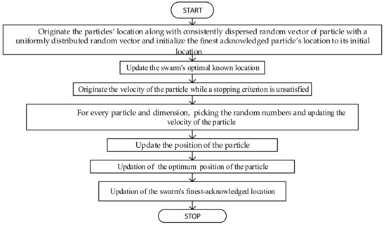
Figure 5.
Flowchart depicting MEEPSO algorithm.
The steps of the algorithm are described below:
- Step 1: for each particle initialize the position of a particle with a uniformly distributed random vector.
- Step 2: initialize the best-acknowledged position of the particle to its initial position, .
- Step 3: if , then update the swarm’s best-known position, .
- Step 4: initialize the velocity of the particle.while a termination criterion is not met.
- Step 5: for each particle and for each dimension , pick random numbers .
- Step 6: update the velocity of the particle,
- Step 7: update the position of the particle.
- Step 8: if , then update the best-known position of the particle
- Step 9: if , then update the swarm’s best-acknowledged position.
The lower and upper limits of the search-space are the values and . The termination principle may be the number of reiterations completed or a solution where a satisfactory objective function value is originated [50,61,64,65]. Being selected by the practitioner, the variables , , and control the behavior and efficacy of the MEEPSO method.
2.7.2. Parameter Choice
The choice of MEEPSO factors may have great influence on optimization performance. Choosing parameters that yield sensible performance has, so far, been the topic of abundant analysis. The MEEPSO parameters can even be tuned by using another overlaying optimizer, a concept called meta-optimization, or perhaps fine-tuned throughout the optimization, such as throughout fuzzy logic. Parameters have been conjointly tuned for various optimization eventualities.
The driving crescendos of every particle separately in the explored space is managed through its present position and velocity that can be observed while using the probable resolution in the problem space, whereby the existing velocity is governed with
- the previous velocity;
- the distance from the position where the particle attained its greatest fitness (personal best, ); and,
- the distance from the particle that accomplished the best fitness among all of the particles (global best, ).
The position of an individual particle is a probable solution, besides the respective particle remembers the best position that it attains throughout the whole optimization process (). The swarm together learns the best position that is attained with every particle ().
The position coupled with the velocity association after the iteration amongst any two entities is attained through the subsequent updating expression:
where = velocity of the particle. This parameter is checked for minimum and maximum limits violation. If is less than the minimum value, then it is fixed at the minimum value, and, if is more than the maximum limit, then it is fixed at the maximum value. and are the acceleration factors and constants. They are not negative constants. They regulate the comparative effect of the peculiar (local) and collective (global) information on the effort of every particle, is the inertia weight or function. , are the autonomous consistently dispersed random variables around the span of (0,1), is the position of the particle. is the greatest preceding position of , is the finest global position that is attained through a particle surrounded by the complete population.
The inertia function, w, stabilizes the local and global explorations throughout the evolution procedure. At large, a huge inertia weight levied by the side of the primary search stages lets the search space be exhaustively discovered. By steadily reducing the inertia weight, further upgraded results are attained in the ultimate search stage. The main aim of this adjustment is to circumvent early convergence in the primary explored phases besides refining convergence to the global best solution throughout the concluding examined phases. The perception of linearly declining inertia weight that is related to MEEPSO is provided by:
where and are the highest and the lowest values of the inertia weight, is the recent number of iterations, and maxiter refers to the highest number of iterations.
2.8. Power World Simulator (PWS):
The Power World Simulator is a platform for power system simulation that is designed from scratch up to be manageable and highly communicating. The simulator has the command for grave engineering investigation, but it is also so collaborating and user friendly that it can be recycled to elucidate power system actions to non-technical spectators. The simulator comprises numerous combined products. At its principal is a complete, vigorous Power Flow Result engine that is skilled in efficiently explaining systems of up to 250,000 buses.
ATC can be determined while using PWS for a normal mode operation for different bus systems (say six bus and 30 bus systems) in the case of normal and line outage contingency mode operation, wherein the thermal limit is taken as constraint and reactive power as constant. ATC may be determined for the bilateral and multilateral transactions. The IEEE 30 bus system comprised six generators and 41 transmission lines [65].
3. Results and Discussion
The procedure implemented for the intensification of ATC in this illustrated work is analyzed on IEEE six bus and 30 bus systems. Regarding the FACTS device, TCSC is optimally located by using the proposed SPCR technique. The MEEPSO algorithm is applied for augmenting ATC after placing TCSC at an optimal location, using MATLAB (R2017b, The Math Works, Inc.,) 64-bit Windows environment. The represented algorithm has been carried out by taking, into account, the count of particles as 50 for maximum iterations of 200, is 1 and is 1.2, and are both 2. The maximum amount of TCSC compensation is 50% and the minimum is 0. The base MVA taken is 100 MVA. All of the parameters are taken in per unit. The values are computed by exercising the ACPTDF procedure. A comparison involving with and without TCSC, exercising the MEEPSO technique is monitored and examined with the DCPTDF technique and the values of ATC are calculated with the help of the upcoming Power World Simulator software (Simulator GOS Education 21 version) and MATLAB both. The work is divided in two components, where the first part consists of optimization of location of FACTS device by the novel Sensitivity and Power loss based Congestion Reduction (SPCR) method and the second part comprises of calculation of maximum value of ATC while using the proposed Metaheuristic Evolutionary Particle Swarm Optimization (MEEPSO) technique.
3.1. Placement and Location Optimization of FACTS Device to Increase the ATC
This case deals with the six bus system and 30 bus system. A standard IEEE system is taken into consideration. The load flow is calculated using the Newton Raphson Method and the base case values of ATC are calculated by the ACPTDF technique in the MATLAB environment. Subsequently, TCSC is optimally placed by using the SPCR technique while considering both the DC power flow sensitivity factor method and the Reactive Power loss reduction method. The placement of FACTS device and its location optimization was accomplished through the following steps:
- calculation of values of DC power flow sensitivity factor;
- evaluation of values of reactive power loss sensitivity index and reactive power losses by placing TCSC;
- comparison of total reactive power losses plus real power losses on sensitive lines;
- judgement of total real power losses after placing TCSC on sensitive lines;
- assessment of real power flows besides reactive and real power losses at different locations of TCSC;
- appraisal of total real power losses after placing TCSC on sensitive lines; and,
- comparison of real power flows at different locations of TCSC.
3.1.1. Case 1: 6 Bus System
When considering the six bus system having three generators and eleven lines, the sensitivity indices for both the methods are calculated and sensitive lines are found. The whole calculations are done under the MATLAB R2017b environment. The reactive power losses, real power losses, and calculated line flow, after placing the TCSC at the location-based upon the two criteria that are listed above, are shown below. The TCSC is used at a 50% compensation level. The outage of line 9 is considered. Table 1 shows the calculated value
.

Table 1.
Calculated values of DC power flow sensitivity factor, .
From Table 1 and applying the DC power flow sensitivity factor method, the lines having the most positive value are sensitive. Hence, the sensitive lines are lines 1, 7, 8, and 11. In this method, the outage of line 9 is considered.
Table 2 shows the calculated values of the reactive power loss sensitivity index. The lines having the most positive values are sensitive, according to the reactive power loss sensitivity index. Lines 1, 4, 10, and 11 are sensitive, according to Table 2.
Table 2.
Calculated values of reactive power loss sensitivity index,
.
Table 3 shows the reactive power losses after placing TCSC in the sensitive lines. The bold values are indicating the reduced reactive power losses (obtained by using TCSC) than the original values of losses (obtained without using TCSC) when the TCSC is placed in the sensitive lines. When TCSC is placed inline 1, reactive power losses are reduced on lines 1, 2, 3, and 4. When it is placed in line 4, the reactive power losses are reduced on lines 1, 2, 4, 8, and 9. Similarly, when TCSC is placed at lines 7 and 8, the reactive power losses are reduced on lines 3, 5, 6, 7, 9, 10, and on lines 2 to 6, 8, to 11, respectively.
Table 3.
Calculation of Reactive power losses by placing TCSC.
After placing TCSC in lines 10 and 11, the reactive power losses became reduced on lines 3, 6, 7, and 10 and lines 2 to 6, 8, 10, and 11 respectively. Table 4 shows the total reactive power losses on these lines. It is clear from Table 4; all sensitive lines contain reduced losses. However, in lines 1, 7, 8, and 11, the total reactive losses are reduced considerably.
Table 4.
Comparison of Total Reactive power losses on sensitive lines.
Table 5, below, shows the real power losses that were calculated on sensitive lines 1, 4, 7, 8, 10, and 11. The real power losses are decreased in lines 1, 2, 3, 4, and 10 when TCSC is placed at line 1. It is decreased in lines 1, 2, 4, 8, 9, and 11 when TCSC is placed at line 4. The real power losses are reduced at lines 3, 5–7, 9, and 10 after placing TCSC at line 7. After placing TCSC at line 8 and 10, the real power losses are reduced at lines 2–6, 8–11, and lines 1, 3 6, 7, 10, respectively. Similarly, it becomes reduced on lines 2, 3, 5, 6, 8, 10, and 11, after placing TCSC in line 11.
Table 5.
Calculation of Real Power Losses at sensitive lines.
The total real power losses are reduced significantly when TCSC is placed at lines 1, 7, 8, 10, and 11 in six-bus system, as is clear from Table 6. The reduction in real power losses in lines is significant in lines 7, 8, and 11.
Table 6.
Comparison of Total Real power losses after placing TCSC on sensitive lines.
Table 7 shows the values of real power flows, after placing TCSC at sensitive lines. The real power flows are considerably reduced when TCSC is placed at lines 1, 7, 8, and 11. When TCSC is placed at line 1, power flow gets decreased at line no. 1, as is clear from Table 7. Similarly, when it is placed in line 7, the real power flows are decreased at lines 7 and 9. When TCSC is placed at line 8, power flow on lines 3, 5, 6, 8, 9, and 10 is decreased and, when placed at line 11, it becomes reduced at lines 6, 8, and 10. The reduction of real power flows suggests that the available transfer capability is increased in these lines. The bold values shown in Table 7 are showing reduced power flows. The remarkable reduction in real power flows is noticed when TCSC is placed at line 7, 8, and 11, as is clear from Table 7. Many lines have observed lesser power flows when TCSC is paced at three lines. This will result in relieving in congestion of these lines and, hence, allow these lines to be able to transfer power more than already committed usage and will also prevent overloading in the future. These results prove the efficacy of the proposed SPCR method in optimally locating the TCSC to relieve congestion.
Table 7.
Comparison of Real Power Flows at different locations of TCSC.
The variation of real power losses for the six-bus system has been represented in the bar graph, as shown in Figure 6. It is evident from the graph that except in line 4, the total real power losses are lesser after placing TCSC as compared with that of without its placement. Among all of the considered lines, the seventh line has witnessed the minimum total real power loss, which is about 6.70 MW.
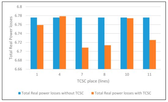
Figure 6.
Comparison of Real Power Losses at different transactions by various methods (six bus system).
3.1.2. Case 2: 30 Bus System
This case deals with the 30 bus system. A standard IEEE system is taken into consideration. The load flow is calculated while using the Newton Raphson Method and the base case values of ATC are calculated by the ACPTDF technique in the MATLAB environment. Subsequently, TCSC is optimally placed by using the SPCR technique while considering both the DC power flow sensitivity factor method and the Reactive Power loss reduction method. Further, the MEEPSO technique is used to enhance ATC after placing TCSC at an optimal location.
When considering the 30 bus system having six generators and forty-one lines, the sensitivity indices for both of the methods are calculated and sensitive lines are found. The whole calculations are done under the MATLAB R2017b environment. The reactive power losses, real power losses, and calculated line flow, after placing the TCSC at the location-based upon the two criteria listed are shown below. The TCSC is used at a 50% compensation level. The outage of line 14 is considered. Table 8 shows the calculated values of
and reactive power loss sensitivity index,
. From this table and applying the DC power flow sensitivity factor method, along with the reactive power loss reduction method, the lines having the most positive value are sensitive. Hence, the sensitive lines are lines 11 and 31 according to the DC power flow sensitivity factor method and lines 12 and 15, according to the Reactive Power loss reduction method. These are the sensitive lines having the most positive values. Table 8 shows the most positive values in bold.
Table 8.
Calculated values of
and
.
Table 9 shows the reactive power losses after placing TCSC in the sensitive lines. The bold values indicate the reduced reactive power losses (obtained by using TCSC) than the original values of losses (obtained without using TCSC) when the TCSC is placed in the sensitive lines. When TCSC is placed in line 11, reactive power losses are reduced on lines 1, 2, 4, 11, 15, 19, 20, and 31. When it is placed in line 12, except line 1, all other lines noticed a reduction in the reactive power losses. Similarly, when TCSC is placed in line 15, except lines 11 and 12, all other lines observed reduced reactive power losses. After placing TCSC in line 31, all of the lines have reduced losses, except lines 11 and 12.
Table 9.
Calculation of Reactive power losses by placing TCSC.
Table 10 shows the total reactive power losses on these lines. On all lines mentioned in Table 10, a decrease in the total reactive power losses is observed. However, when TCSC is placed in lines 11 and 12, the decrease in total reactive power losses is much more significant.
Table 10.
Comparison of Total Reactive power losses on sensitive lines.
Table 11 shows the real power losses that were calculated on sensitive lines 11, 12, 15, and 31. The real power losses are decreased on all lines when TCSC is placed in line 11. It is decreased on all lines, except line 1, when TCSC is placed in line 12. The real power losses are reduced at all lines, except lines 11 and 12, after placing TCSC at line 15 and 31.
Table 11.
Calculation of Real Power Losses at sensitive lines.
The total real power losses are reduced significantly when TCSC is placed at lines 11, 12, 15, and 31, as is clear from Table 12. The reduction in real power losses is significant in line 12, as is evident from Table 12.
Table 12.
Comparison of Total Real power losses after placing TCSC on sensitive lines.
Table 13 shows the values of real power flows, after placing TCSC at sensitive lines. The real power flows are reduced considerably when TCSC is placed at lines 11, 12, 15, and 31. When TCSC is placed at line 11, power flow becomes decreased at all lines, except line 4, as is clear from Table 13. Similarly, when it is placed in line 12, the real power flows are decreased at all lines, except in line 1. When TCSC is placed at lines 15 and 31, power flow on all lines is decreased, except lines 4, 11, and 12. The reduction of real power flows suggests that the available transfer capability is increased in the lines having less real power flows.
Table 13.
Comparison of Real Power Flows at different locations of TCSC.
The bold values shown in Table 13 depict reduced power flows. The remarkable reduction in real power flows is noticed when TCSC is placed at lines 11, 12, 15, and 31, as is clear from Table 13. Many lines observed lesser power flows. This will result in relieving in congestion of these lines and, hence, allow for these lines to be able to transfer power more than already committed usage and will also prevent overloading in the future. These results prove the efficacy of the proposed SPCR method in optimally locating the TCSC to relieve congestion.
Figure 7 represents the bar graph of comparison of real power losses for 30-bus system. It is clear in the graph that in all the cases, the total real power losses are lesser after the placement of TCSC as compared to that without placing it. Among all of the considered cases, the 12th line has witnessed the minimum total real power loss, which is about 9.048 MW.
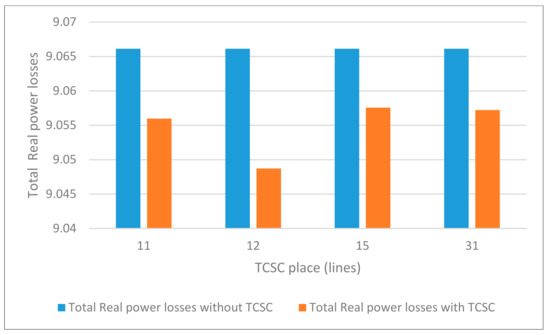
Figure 7.
Comparison of total real power loss at different lines by various methods (30 bus system)
3.2. Calculation of Enhanced ATC
The ATC was optimized and calculated with the help of the MEEPSO technique, which comprises of the following steps:
- Definition of input parameters in the MEEPSO and initialization of velocity.
- Setting the maximum limit of TCSC compensation and velocity.
- Calculation of ATC.
- Calculation of fitness function and objective function.
- Calculation of particle best position and global best position.
3.2.1. Case 1: 6 Bus System
Figure 8 shows the calculated values of Available Transfer Capability. The values are calculated first for the base case at lines 2–3, 2–5, and 2–6. Transaction T1 means that the transaction is done between buses 2 and 3, transaction T2 means the transaction is done amongst buses 2 and 5, and transaction T3 implies that the transaction is performed for buses 2 and 6. The base case values are calculated using the Newton–Raphson method (for calculating load flow) and the ACPTDF method for finding ATC at all transactions. The ATC is also calculated using the DCPTDF technique. Both of the methods are evaluated with the help of MATLAB and they are further compared with the calculated values of ATC using PWS. The six bus system is first modeled in PWS, taking the same data as in MATLAB. Subsequently, ATC is calculated, and the results are verified with that of ACPTDF and DCPTDF method.
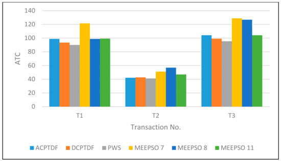
Figure 8.
Comparison of Available Transfer Capabilities (ATC) values at different transactions by various methods (6 bus system).
In order to prove the efficacy of the proposed SPCR and MEEPSO method, the TCSC is placed at lines 7, 8, and 11 (optimal location calculated using SPCR method) and ATC is then calculated using the MEEPSO technique at all transactions. The represented MEEPSO algorithm has been carried out by taking into account the count of particles as 50 for maximum iterations of 200, is 1 and is 1.2, and are both 2. The maximum amount of TCSC compensation is 50% and the minimum is 0. The base MVA taken is 100 MVA. All of the parameters are taken in per unit. Figure 6 shows the comparison of ATC values that were calculated using the MEEPSO technique with the evaluated results of ACPTDF, DCPTDF, and PWS software. Here, MEEPSO 7 means that ATC is calculated using the MEEPSO technique while placing TCSC at line 7, MEEPSO 8 means that the ATC is calculated while using the MEEPSO technique while placing TCSC at line 8 and MEEPSO 11 means that ATC is calculated using MEEPSO technique while placing TCSC at line 11. Figure 6 clearly shows the enhanced values of ATC by using the proposed SPCR and MEEPSO techniques. The validation and efficacy of proposed methods are proved by comparing the results with conventional methods of ACPTDF AND DCPTDF technique. Additionally, the results are further verified using the values that were observed through PWS software.
The comparison reveals the improvement in values of ATC (in MW) by 25.85% by using the currently developed MEEPSO method compared with that of DCPTDF in 6 bus system, whereas it showed an improvement of 9.34% as compared to ACPTDF. The efficacy of the developed method has been proved by taking various transactions between different buses. In six bus systems, ATC has improved remarkably with the currently developed MEEPSO technique when TCSC was placed at line 7 during transaction T1.
3.2.2. Case 2: 30 Bus System
Figure 9 shows the calculated values of Available Transfer Capability. The values are calculated first for the base case in lines 11–25 and 9–11. Transaction T1 means that the transaction is done between buses 11 and 25 and transaction T2 means that the transaction is done amongst buses 9 and 11. The base case values are calculated while using the Newton Raphson method (for calculating load flow) and the ACPTDF method for finding ATC at all transactions. The ATC is also calculated while using the DCPTDF technique. Both of the methods are evaluated with the help of MATLAB and are further compared with the calculated values of ATC using PWS. The six bus system is first modeled in PWS, taking the same data as in MATLAB. Subsequently, ATC is calculated and the results are verified with that of ACPTDF and DCPTDF method.
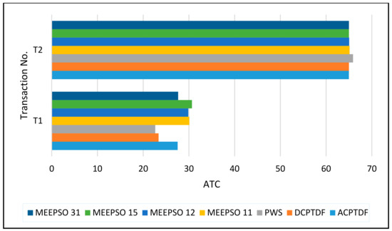
Figure 9.
Comparison of ATC values at different transactions by various methods (30 bus system).
The TCSC is placed at lines 11, 12, 15, and 31 (optimal location calculated while using SPCR method) and then ATC is calculated using the MEEPSO technique at all transactions, in order to prove the efficacy of the proposed SPCR and MEEPSO method. The represented MEEPSO algorithm has been carried out by taking into account the count of particles as 50 for maximum iterations of 200, is 1 and is 1.2, , and are both 2. The maximum amount of TCSC compensation is 50% and the minimum is 0. The base MVA taken is 100 MVA. All of the parameters are taken in per unit. Figure 6 shows the comparison of ATC values that were calculated using the MEEPSO technique with the evaluated results of ACPTDF, DCPTDF, and PWS software. Here, MEEPSO 11 means that ATC is calculated using MEEPSO technique while placing TCSC at line 11, MEEPSO 12 means that the ATC is calculated using the MEEPSO technique while placing TCSC at line 12, MEEPSO 15 means that ATC is calculated using the MEEPSO technique while placing TCSC at line 15, and MEEPSO 31 means that ATC is calculated while using the MEEPSO technique while placing TCSC at line 31. Figure 9 clearly shows the enhanced values of ATC by using the proposed SPCR and MEEPSO technique. The validation and efficacy of proposed methods are proved by comparing the results with the conventional methods of ACPTDF AND DCPTDF technique. Additionally, the results are further verified by using the values that were observed through PWS software.
Similarly, during transactions T2 and T3, the maximum value of ATC (in MW) was observed for the location of TCSC at line 8 and 7, respectively. The results so obtained that have been achieved are more standardized and error-free as compared to those done by conventional methods. In the case of the 30-bus system, a 34.8% improvement in ATC values has been observed while using the MEEPSO technique when compared with the ACPTDF, while it was 33.06% more than that of in DCPTDF.
When the values are manually retrieved from a program, there are great chances of error (Gross Error,), whereas, when the optimization is done with the help of algorithm, not only the chances of gross error get reduced, but also the precision and accuracy of results are achieved. This in turn enhances the overall speed and reliability of the devised method due to its standardization. That is why the two separate algorithms that were previously being used by the researchers are combined in the present study, such that the results can be achieved in single execution.
An attempt has been made to simplify the man machine interface that has enhanced the accessibility of the devised method.
4. Conclusions
In this study, the SPCR method of optimally locating the TCSC and MEEPSO method for calculating ATC have been devised successfully. The IEEE six bus and 30 bus cases are taken for validating the results. The factors considered for the optimization of location in this investigation included DC power flow sensitivity factor, reactive power loss sensitivity index, reactive power losses, real power losses, and real power flows were calculated in SPCR method. Whereas, the values of ATC were obtained by the MEEPSO technique and they are compared with that of ACPTDF, DCPTDF, and PWS. The comparison reveals the improvement in values of ATC by 25.85% than that of DCPTDF in the six bus system by using the currently developed MEEPSO method, whereas it showed an improvement of 9.34% when compared to ACPTDF. The efficacy of the developed method has been proved by taking various transactions between different buses. In six bus systems, ATC has improved remarkably with the currently developed MEEPSO technique when TCSC was placed at line 7 during transaction T1.
Similarly, during transactions T2 and T3, the maximum value of ATC was observed for the location of TCSC at line 8 and 7, respectively. The results so obtained have been achieved by the single execution are more standardized and error free as compared to those that were done by conventional methods. In the case of the 30-bus system, a 34.8% improvement in ATC values has been observed while using MEEPSO technique as compared with the ACPTDF, while it was 33.06% more than that of in DCPTDF. Hence, the use of the proposed technique yielded more promising results when compared with the conventional methods.
5. Future Scope
The proposed methods can be used to find out the dynamic ATC. It can be effectively calculated with the help of transient stability analysis while using PWS software. Additionally, optimal power flow can be analyzed by calculating the cost of placing TCSC at the observed optimal locations. The costs can be calculated by increasing the number of transactions between buses and then performing a comparison. Moreover, different systems can be differentiated by dividing them into separate zones and areas and then comparing their ATC values and costs.
Author Contributions
D.G. has done this work and prepared the manuscript under the supervision of S.K.J. All authors have read and agreed to the published version of the manuscript.
Funding
This research received no external funding.
Institutional Review Board Statement
Not Applicable.
Informed Consent Statement
Not Applicable.
Data Availability Statement
Not Applicable.
Conflicts of Interest
The authors declare no conflict of interest.
Nomenclature
| Abbreviation | Full Form |
| ATC | Available Transfer Capability |
| FACTS | Flexible A.C. Transmission Systems |
| SPCR | Sensitivity and Power loss-based Congestion reduction method |
| MEEPSO | Metaheuristic Evolutionary Particle Swarm Optimization |
| TCSC | Thyristor Controlled Series Compensator |
| TTC | Total Transfer Capability |
| TRM | Transmission Reliability Margin |
| CBM | Capacity Benefit Margin |
| ETC | Existing Transmission Commitment |
| ACPTDF | AC Power Transfer Distribution Factor |
| NATC | Non-recallable ATC |
| RATC | Recallable ATC |
| TCSC reactance | |
| AC Power Transfer Distribution Factor for the line between buses i and j when a transaction is taking place between buses m and n | |
| Available Transfer Capability between buses m and n | |
| DCPTDF | DC Power Transfer Distribution Factor |
| complex power flowing between bus i and j | |
Real complex power flowing between bus i and j | |
Imaginary complex power flowing between bus i and j | |
| the voltage at the bus | |
| the current flowing between buses i and j | |
| change in real power | |
| incremental change in real power concerning the change in angle | |
| change in voltage angle | |
| Mismatch vector of change in power at bus m | |
| Mismatch vector of change in power at bus n | |
| Transacted power | |
| Full Jacobian in polar coordinates | |
| The maximum thermal limit of the line ij | |
| The minimum thermal limit of the line ij | |
| Maximum transfer limit values for each line in the system | |
| PTDF | Power Transfer Distribution Factor |
References
- Kumar, A. Available Transfer Capability Determination and Congestion Management in Competitive Electricity Markets; Indian Institute of Technology: Kanpur, India, 2003. [Google Scholar]
- Mohammed, O.O.; Mustafa, M.W.; Mohammed, D.S.S.; Otuoze, A.O. Available transfer capability calculation methods: A comprehensive review. Int. Trans. Electr. Energy Syst. 2019, 29. [Google Scholar] [CrossRef]
- Rama Susmitha, K.; Rao, G.S. Determination of ATC by using DCPTDF and ACPTDF methods. Int. J. Appl. Eng. Res. 2017, 12, 339–344. [Google Scholar]
- Grijalva, S.; Sauer, P.W.; Weber, J.D. Enhancement of linear ATC calculations by the incorporation of reactive power flows. IEEE Trans. Power Syst. 2003, 18, 619–624. [Google Scholar] [CrossRef]
- Dobson, I.; Greene, S.; Rajaraman, R.; DeMarco, C.L.; Alvarado, F.L.; Zimmerman, R. Electric Power Transfer Capability: Concepts, Applications, Sensitivity, Uncertainty; PSERC: Phillips Hall Ithaca, NY, USA, 2001. [Google Scholar]
- Hojabri, M.; Hizam, H.; Mariun, N.; Abdullah, S.M. Comparative analysis of ATC probabilistic methods. J. Am. Sci. 2010, 6, 4–7. [Google Scholar]
- Albatsh, F.M.; Mekhilef, S.; Ahmad, S.; Mokhlis, H.; Hassan, M.A. Enhancing power transfer capability through flexible AC transmission system devices: A review. Front. Inf. Technol. Electron. Eng. 2015, 16, 658–678. [Google Scholar] [CrossRef]
- Magaji, N.; Mustafa, M.W.; Muda, Z.B. Determination of best location of UPFC device for damping oscillation. Eur. J. Sci. Res. 2010, 41, 203–211. [Google Scholar]
- Hassan, M.O.; Cheng, S.J.; Zakaria, Z.A. Staedy state modeling of static synchronous compensator and thyristor control series compensator for power flow analysis. Inf. Technol. J. 2009, 8, 347–353. [Google Scholar] [CrossRef]
- Ghawghawe, N.D.; Thakre, K.L. Computation of TCSC reactance and suggesting criterion of its location for ATC improvement. Electr. Power Energy Syst. 2009, 31, 86–93. [Google Scholar] [CrossRef]
- Rashidinejad, M.; Farahmand, H.; Fotuhi-firuzabad, M.; Gharaveisi, A.A. ATC enhancement using TCSC via artificial intelligent techniques. Electr. Power Syst. Res. 2008, 78, 11–20. [Google Scholar] [CrossRef]
- Gaur, D.; Mathew, L. Optimal placement of FACTS devices using optimization techniques: A review. IOP Conf. Ser. Mater. Sci. Eng. 2018, 331. [Google Scholar] [CrossRef]
- Huang, G.M.; Yan, P. TCSC and SVC as Re-dispatch tools for congestion management and TTC improvement. In Proceedings of the 2002 IEEE Power Engineering Society Winter Meeting, New York, NY, USA, 27–31 January 2002; Volume 1, pp. 660–665. [Google Scholar]
- Pankajam, T.P.; Srinivasa, R.J.; Amarnath, J. ATC enhancement with FACTS devices considering reactive power flows using PTDF. Int. J. Electr. Comput. Eng. 2013, 3, 741–750. [Google Scholar] [CrossRef]
- Ou, Y.; Singh, C. Improvement of total transfer capability using TCSC and SVC. Proc. IEEE Power Eng. Soc. Transm. Distrib. Conf. 2001, 2, 944–948. [Google Scholar] [CrossRef]
- Yadav, N.K. Implementation of FACTS device for enhancement of ATC using PTDF. Int. J. Comput. Electr. Eng. 2011, 3, 343–348. [Google Scholar] [CrossRef]
- Schnurr, N.; Wellssow, W.H. Determination and enhancement of the available transfer capability in FACTS. 2001 IEEE Porto Power Tech Proc. 2001, 4, 34–39. [Google Scholar] [CrossRef]
- Gupta, S.K.; Singh, M.; Sharma, H.D. Enhancement of ATC using UPFC under deregulated environment. J. Power Electron. Power Syst. 2016, 6, 66–72. [Google Scholar]
- Alam, A.; Abido, M.A. Parameter optimization of shunt FACTS controllers for power system transient stability improvement. In Proceedings of the 2007 IEEE Lausanne Power Tech, Lausanne, Switzerland, 1–5 July 2007; pp. 1–6. [Google Scholar]
- Nireekshana, T.; Rao, G.K.; Raju, S.S. Available transfer capability enhancement with FACTS using Cat Swarm Optimization. Ain Shams Eng. J. 2016, 7, 159–167. [Google Scholar] [CrossRef]
- Luo, X.; Patton, A.D.; Singh, C. Real power transfer capability calculations using multi-layer feed-forward neural networks. IEEE Trans. Power Syst. 2000, 15, 903–908. [Google Scholar] [CrossRef]
- Pandey, S.N.; Pandey, N.K.; Tapaswi, S.; Srivastava, L. Neural network-based approach for ATC estimation using distributed computing. IEEE Trans. Power Syst. 2010, 25, 1291–1300. [Google Scholar] [CrossRef]
- Jain, T.; Singh, S.N.; Srivastava, S.C. Fast static available transfer capability determination using radial basis function neural network. Appl. Soft Comput. J. 2011, 11, 2756–2764. [Google Scholar] [CrossRef]
- Zhang, Q.; Benveniste, A. Wavelet networks. IEEE Trans. Neural Netw. 1992, 3, 889–898. [Google Scholar] [CrossRef]
- Zhang, J.; Walter, G.G.; Miao, Y.; Ngai, W.; Lee, W. Wavelet neural networks for function learning. IEEE Trans. Signal Process. 1995, 43, 1485–1497. [Google Scholar] [CrossRef]
- Billings, S.A.; Wei, H. A new class of wavelet networks for nonlinear system identification. IEEE Trans. Neural Netw. 2005, 16, 862–874. [Google Scholar] [CrossRef]
- Ma, X.W. Overview and literature survey of fuzzy set theory in power systems. IEEE Trans. Power Syst. 1995, 10, 1676–1690. [Google Scholar]
- Jang, J.-S.R.; Sun, C.-T.; Mizutani, E. Neuro-Fuzzy and Soft Computing; a Computational Approach to Learning and Machine Intelligence, 6th ed.; Prentice-Hall: Upper Saddle River, NJ, USA, 1997. [Google Scholar]
- Zimmermann, H.J. Fuzzy programming and linear programming with several objective functions. Fuzzy Sets Syst. 1978, 1, 45–55. [Google Scholar] [CrossRef]
- Miranda, V.; Saraiva, J.T. Fuzzy modelling of power system optimal load flow. IEEE Trans. Power Syst. 1992, 7, 843–849. [Google Scholar] [CrossRef]
- Ramesh, V.C.; Li, X. A fuzzy multiobjective approach to contingency constrained OPF. IEEE Trans. Power Syst. 1997, 12, 1348–1354. [Google Scholar] [CrossRef]
- Khairuddin, A.B.; Ahmed, S.S.; Mustafa, M.W.; Zin, A.A.M.; Ahmad, H. A novel method for ATC computations in a large-scale power system. IEEE Trans. Power Syst. 2004, 19, 1150–1158. [Google Scholar] [CrossRef]
- Kim, S.; Kim, M.K.; Park, J. Consideration of multiple uncertainties for evaluation of available transfer capability using fuzzy continuation power flow. Electr. Power Energy Syst. 2008, 30, 581–593. [Google Scholar] [CrossRef]
- Hahn, T.K.; Kim, M.K.; Hur, D.; Park, J.; Yoon, Y.T. Evaluation of available transfer capability using fuzzy multi-objective contingency-constrained optimal power flow. Electr. Power Syst. Res. 2008, 78, 873–882. [Google Scholar] [CrossRef]
- Lai, L.L.; Ma, J.T.; Yokoyama, R.; Zhao, M. Improved genetic algorithms for optimal power flow under both normal and contingent operation states. Electr. Power Energy Syst. 1997, 19, 287–292. [Google Scholar] [CrossRef]
- Paranjothi, S.R.; Anburaja, K. Optimal power flow using refined genetic algorithm. Electr. Power Compon. Syst. 2002, 30, 1055–1063. [Google Scholar] [CrossRef]
- Devaraj, D.; Yegnanarayana, B. Genetic-algorithm-based optimal power flow for security enhancement. IEE Proc.-Gener. Transm. Distrib. 2005, 152, 899–905. [Google Scholar] [CrossRef]
- Bakirtzis, A.G.; Biskas, P.N.; Zoumas, C.E.; Petridis, V. Optimal power flow by enhanced genetic algorithm. IEEE Trans. Power Syst. 2002, 17, 229–236. [Google Scholar] [CrossRef]
- Yuryevich, J.; Wong, K.P. Evolutionary programming based optimal power flow algorithm. IEEE Trans. Power Syst. 1999, 14, 1245–1250. [Google Scholar] [CrossRef]
- Gan, D.; Thomas, R.J.; Zimmerman, R.D. Stability-constrained optimal power flow. IEEE Trans. Power Syst. 2000, 15, 535–540. [Google Scholar] [CrossRef]
- Chen, L.; Tada, Y.; Okamoto, H.; Tanabe, R.; Ono, A. Optimal operation solutions of power systems with transient stability constraints. IEEE Trans. Circuits Syst. I Fundam. Theory Appl. 2001, 48, 327–338. [Google Scholar] [CrossRef]
- Richter, C.W.; Sheble, G.B. Genetic algorithm evolution of utility bidding strategies for the competitive marketplace. IEEE Trans. Power Syst. 1998, 13, 256–261. [Google Scholar] [CrossRef]
- Richter, C.W.; Sheble, G.B.; Ashlock, D. Comprehensive bidding strategies with genetic programming/finite state automata. IEEE Trans. Power Syst. 1999, 14, 1207–1212. [Google Scholar] [CrossRef]
- Gountis, V.P.; Bakirtzis, A.G. Bidding strategies for electricity producers in a competitive electricity marketplace. IEEE Trans. Power Syst. 2004, 19, 356–365. [Google Scholar] [CrossRef]
- Othman, M.M.; Mohamed, A.; Hussain, A. Available transfer capability assessment using evolutionary programming based capacity benefit margin. Int. J. Electr. Power Energy Syst. 2006, 28, 166–176. [Google Scholar] [CrossRef]
- Abido, M.A. Optimal power flow using particle swarm optimization. Electr. Power Energy Syst. 2002, 24, 563–571. [Google Scholar] [CrossRef]
- Mo, N.; Zou, Z.Y.; Chan, K.W.; Pong, T.Y.G. Transient stability constrained optimal power flow using particle swarm optimisation. IET Gener. Transm. Distrib. 2007, 1, 476–483. [Google Scholar] [CrossRef]
- Yumbla, P.E.O.; Ramirez, J.M.; Coello Coello, C.A. Optimal power flow subject to security constraints solved with a particle swarm optimizer. IEEE Trans. Power Syst. 2008, 23, 33–40. [Google Scholar] [CrossRef]
- Zhao, B.; Guo, C.X.; Cao, Y.J. A multiagent-based particle swarm optimization approach for optimal reactive power dispatch. IEEE Trans. Power Syst. 2005, 20, 1070–1078. [Google Scholar] [CrossRef]
- Clerc, M.; Kennedy, J. The particle swarm—Explosion, stability, and convergence in a multidimensional complex space. IEEE Trans. Evol. Comput. 2002, 6, 58–73. [Google Scholar] [CrossRef]
- Farahmand, H.; Rashidinejad, M.; Gharaveici, A.A.; Shojaee, M. An application of hybrid heuristic approach for ATC enhancement. In Proceedings of the 2006 Large Engineering Systems Conference on Power Engineering, Halifax, NS, Canada, 26–28 July 2006; pp. 125–130. [Google Scholar]
- Karthiga, M.M.; Raja, S.C.; Venkatesh, P. Enhancement of available transfer capability using TCSC devices in deregulated power market. In Proceedings of the International Conference on Innovations in Power and Advanced Computing Technologies [i-PACT2017], Vellore, India, 21–22 April 2017; Volume 17, pp. 1–7. [Google Scholar]
- Farahmand, H.; Masoud, R.; Akbar, G.A. A combinatorial approach of real GA & Fuzzy to ATC enhancement. Turkey J. Electr. Eng. 2007, 1, 77–88. [Google Scholar]
- Esmaili, H.; Ramezani, Y.; Hemmatyar, A.M.A. ATC enhancement using SSSC, a case study of harmony search vs PSO. J. Basic Appl. Sci. Res. 2012, 2, 3416–3425. [Google Scholar]
- Sudheer, T.S.; Kakinada, J.; Ananthapur, J. Optimal location of the facts devices using the sensitivity approach for the enhancement of ATC and voltage profile in deregulated power system. Int. J. Comput. Appl. 2013, 76, 32–38. [Google Scholar]
- Mat, N.; Othman, M.M.; Musirin, I.; Mohamed, A.; Hussain, A. Determination of Available Transfer Capability (ATC) Considering Integral Square Generator Angle (ISGA). In Proceedings of the 2nd WSEAS International Conference on Circuits, Systems, Signal and Telecommunications (CISSTș08), Systems, Acapulco, Mexico, 25–27 January 2008; pp. 126–131. [Google Scholar]
- Ramezani, M.; Member, S.S.; Haghifam, M.; Member, S.S.; Singh, C.; Seifi, H.; Moghaddam, M.P. Determination of capacity benefit margin in multiarea power systems using particle swarm optimization. IEEE Trans. Power Syst. 2009, 24, 631–641. [Google Scholar] [CrossRef]
- Tsai, C.Y.; Lu, C.N. Bootstrap application in ATC estimation. IEEE Power Eng. Rev. 2001, 21, 40–42. [Google Scholar] [CrossRef]
- Shi, Y.; Eberhart, R. A modified particle swarm optimizer. In Proceedings of the IEEE International Conference on Evolutionary Computiation, Anchorage, AK, USA, 20–22 May 1998; pp. 69–73. [Google Scholar]
- Eberhart, R.; Kennedy, J. Particle swarm optimization. Proc. IEEE Int. Conf. Neural Networks 1995, 21, 1942–1948. [Google Scholar] [CrossRef]
- Kennedy, J. Particle swarm: Social adaptation of knowledge. Proc. IEEE Conf. Evol. Comput. ICEC 1997, 303–308. [Google Scholar] [CrossRef]
- Kennedy, J.; Eberhart, R.C. Swarm Intelligence, 1st ed.; Morgan Kaufmann: Burlington, MA, USA, 2001. [Google Scholar]
- Poli, R. An Analysis of Publications on Particle Swarm Optimisation Applications; Department of Computer Science, University of Essex: Colchester, UK, 2017. [Google Scholar]
- Poli, R. Analysis of the publications on the applications of particle swarm optimisation. J. Artif. Evol. Appl. 2008, 2008. [Google Scholar] [CrossRef]
- Bonyadi, R.M.; Michalewicz, Z. Particle swarm optimization for single objective continuous space problems: A review mohammad. Evol. Comput. 2017, 25. [Google Scholar] [CrossRef] [PubMed]
Publisher’s Note: MDPI stays neutral with regard to jurisdictional claims in published maps and institutional affiliations. |
© 2021 by the authors. Licensee MDPI, Basel, Switzerland. This article is an open access article distributed under the terms and conditions of the Creative Commons Attribution (CC BY) license (http://creativecommons.org/licenses/by/4.0/).