Research on the Speed Sliding Mode Observation Method of a Bearingless Induction Motor

Abstract

In order to achieve the speed sensorless control of a bearingless induction motor (BL-IM), a novel sliding mode observation (SMO) method of motor speed is researched. First of all, according to the mathematical model of a BL-IM system, the observation model of stator current and that of rotor flux-linkage are derived. In order to overcome the chattering problem of a sliding mode observer, a continuous saturation function is adopted to replace the traditional sign function. Then, the SMO model of motor speed is derived, and the stability of the proposed motor speed SMO method is validated by the Lyapunov stability theory. At the end, the observed motor speed and rotor flux-linkage are applied to a BL-IM inverse “dynamic decoupling control” (DDC) system. Simulation results show that the real-time observation or dynamic tracking of motor speed and rotor flux-linkage are achieved in a more timely manner and more accurately, and higher steady-state observation accuracy is obtained; the proposed SMO method can be used in the BL-IM’s inverse DDC system to realize reliable magnetic suspension operation control without a speed sensor.

1. Introduction

To meet the need for high-speed drive in the industrial field, the alternating current (AC) motor supported by all kinds of magnetic bearings is widely researched and developed [1,2,3,4,5], but it still has some obvious disadvantages, such as a limited critical speed and more magnetic suspension system power consumption, etc. [1,6,7,8,9]. The bearingless motor (BLM) is a new AC motor [1,10,11,12,13,14,15] proposed based on the similar structure between an ordinary AC motor stator and a magnetic bearing. Under normal circumstances, two sets of windings are embedded in the BLM stator, including a set of torque windings with pole-pair number p₁ and current frequency ω₁, and a set of suspension windings with pole-pair number p₂ and current frequency ω₂. When the pole-pair numbers and current frequencies of the two sets of stator windings meet the “p₂ = p₁ ± 1, ω₂ = ω₁” qualifications, the controllable magnetic suspension force and electromagnetic torque can be produced simultaneously [1,7,16,17,18,19,20]. The controllable magnetic suspension force’s generation principle is shown in Figure 1 [15,19], where the p₁ and p₂ equal to 2 and 1, respectively. Compared with a magnetic bearing motor, the BLM has unique advantages, such as a shorter shaft and a higher critical speed, etc., giving it bright application prospects in the high-speed-drive field [1,10,11,21,22,23,24,25]. In all kinds of BLMs, because of the robust structure and larger stiffness coefficient of magnetic suspension force, the bearingless induction motor (BL-IM) has aroused wide attention [1,6,7,8,9,12,13,26,27,28].

As for a BL-IM, during the process of magnetic suspension operation, accurate motor speed information is needed. The mechanical speed sensor will increase the system cost and the axial length of a BL-IM. In addition, its performance is easily affected by the environment. Therefore, in the future application of a BL-IM, speed sensorless technology is one of the bottlenecks. For an ordinary AC motor, speed sensorless technology has been widely studied. The adopted methods include the direct calculation method [29], model reference adaptive system (MRAS) method [30], extended Kalman filter (EKF) method [31], adaptive full order observer [32], the high frequency signal injection (HFSI) method [33], and the sliding mode observation (SMO) method [34]. Regarding the speed/position sensorless technology of a BLM system, some studies have been carried out, most of which refer to the research ideas of an ordinary AC motor.

The observation accuracy of the MRAS method is greatly affected by the accuracy of the reference model [30], but it is easy to implement, so it has aroused more attention in the BLM field [35,36]. In order to solve the problems of cumulative error and initial integral value caused by pure integrators in the traditional MRAS speed observer, reference [35] combined “improved generalized second-order integrator” with phase-locked loop to replace pure integrator, which effectively improved the speed observation accuracy of a BL-IM system. In a d-q synchronous coordinate system, reference [36] established an adjustable model of reactive power containing estimated speed, and realized the MRAS speed observation of a BL-IM. Since the EKF method has the advantages of strong anti-noise interference ability [31], it has also attracted attention in the field of BLMs. In reference [37], the terminal voltage and stator current of a BL-IM are taken as control variables and measurable variables, respectively. The observation algorithm of motor speed is obtained through the recursive formula of EKF. In reference [38], a cascaded Kalman filter is proposed for a BL-IM, the volatile motor parameters are used as a state vector in the system model; after the obtained motor parameter values are feed-backed to the identification algorithm, the speed identification is achieved, and the influence of motor parameter change is effectively reduced. In reference [39], a speed estimation method based on an iterative-center-difference Kalman filter (ICDKF) is put forward. Based on the analysis of the BL-IM mathematical model, the model error is reduced by using the Sterling interpolation formula in the filter, and the filtering accuracy is improved by iteration. Finally, the filter is used to estimate the speed online. The advantage of this method is that it can reduce the influence of load disturbance on speed estimation. But the calculation of the EKF method is complex and there are a lot of random parameters to be debugged, so it is not convenient for engineering applications. The speed observation based on the HFSI method is less affected by motor parameters, but it requires that the motor structure has certain salient-pole characteristics, which is more suitable for permanent magnet motor and switched reluctance motor, but less used in the induction motor. In reference [40], to avoid the skin effect of the rotor bar caused by a high-frequency carrier signal, based on a low-frequency signal injection method, and combined with the BL-IM fundamental wave model, a speed self-detection method is proposed. The speed observer based on the signal injection method has strong robustness, but its signal extraction algorithm is complex. In reference [41], a speed observation scheme based on an artificial-neural-network (ANN) inverse system is proposed for a BL-IM by cascading the original torque subsystem and its neural network inverse system; the speed was observed successfully. The speed identification method based on artificial intelligence can obtain strong robustness to noise interference, but its implementation algorithm is complex and its practical application is difficult. The SMO method has low requirements for the motor’s mathematical model, and it can obtain good dynamic observation characteristics in a wide speed range. Therefore, it has a bright application prospect in the BLM speed observation field. Now, aiming at BLM, there are some preliminary study results on the speed SMO method, but they mainly focus on the permanent magnet type BLM. In reference [42], a rotor position detection algorithm based on the SMO method was established for a multiphase permanent magnet BLM, and a low-pass filter varying with speed was designed, which effectively suppressed the disturbance of magnetic suspension control current on the motor speed. As for a BL-IM, a sliding mode control method is put forward in reference [25], but the speed SMO method has not been reported.

In this paper, a novel motor speed SMO method of a BL-IM is proposed. Firstly, the observation model of stator current and that of rotor flux-linkage are derived, and then the SMO model of moor speed is derived. The identified speed and rotor flux-linkage are used in the BL-IM inverse “dynamic decoupling control” (DDC) system. The stability of the proposed observation method is proved based on the stability theory of Lyapunov. Simulation results show that the proposed SMO method for BL-IM has higher observation accuracy and faster dynamic tracking speed for rotor flux-linkage and motor speed, which can be used in the BL-IM speed sensorless inverse DDC system, and can realize its reliable magnetic suspension operation control.

2. Mathematical Model of Sliding Mode Observer for a BL-IM

2.1. SMO Models of Stator Current and Rotor Flux-Linkage

Definition: α-β is a stationary two-phase coordinate system whose α-axis is located at the axis of A-phase torque winding. Then, in α-β coordinate system, the torque system dynamic model can be expressed as follows [25,28]:

$$\{\begin{array}{c}p{i}_{s1\alpha }=-\frac{R_{s1}{L}_{r1}^2+R_{r1}{L}_{m1}^2}{\sigma L_{s1}{L}_{r1}^2}{i}_{s1\alpha }+\frac{L_{m1}}{\sigma L_{s1}{L}_{r1}{T}_{r1}}{\psi }_{r1\alpha }+\frac{L_{m1}}{\sigma L_{s1}{L}_{r1}}{\omega }_r{\psi }_{r1\beta }+\frac{u_{s1\alpha }}{\sigma L_{s1}}\hfill \\ p{i}_{s1\beta }=-\frac{R_{s1}{L}_{r1}^2+R_{r1}{L}_{m1}^2}{\sigma L_{s1}{L}_{r1}^2}{i}_{s1\beta }-\frac{L_{m1}}{\sigma L_{s1}{L}_{r1}}{\omega }_r{\psi }_{r1\alpha }+\frac{L_{m1}}{\sigma L_{s1}{L}_{r1}{T}_{r1}}{\psi }_{r1\beta }+\frac{u_{s1\beta }}{\sigma L_{s1}}\hfill \\ p{\psi }_{r1\alpha }=\frac{L_{m1}}{T_{r1}}{i}_{s1\alpha }-\frac{1}{T_{r1}}{\psi }_{r1\alpha }-{\omega }_r{\psi }_{r1\beta }\hfill \\ p{\psi }_{r1\beta }=\frac{L_{m1}}{T_{r1}}{i}_{s1\beta }+{\omega }_r{\psi }_{r1\alpha }-\frac{1}{T_{r1}}{\psi }_{r1\beta }\hfill \end{array}$$

(1)

where, u_s1α and u_s1β are stator voltage components; i_s1α and i_s1β are stator current components; ψ_r1α and ψ_r1β are rotor flux-linkage components; $\sigma =1-L_{m1}^2/L_{s1}{L}_{r1}$, $T_{\mathrm{r}1}=L_{r1}/R_{r1}$, the L_s1, L_r1 and L_m1 are the parameters of stator self-inductance, rotor self-inductance and mutual inductance; ω_r is motor speed; R_r1 is rotor resistance; and p is a differential operator.

From (1), the expressions of rotor flux-linkage and stator current can be simplified as follows:

$$\left[\begin{array}{c}p{i}_{s1\alpha }\\ p{i}_{s1\beta }\end{array}\right]=k_1\left(\left[\begin{array}{cc}\delta & {\omega }_r\\ -{\omega }_r& \delta \end{array}\right]\left[\begin{array}{c}{\psi }_{r1\alpha }\\ {\psi }_{r1\beta }\end{array}\right]-\delta L_{m1}\left[\begin{array}{c}{i}_{s1\alpha }\\ i_{s1\beta }\end{array}\right]\right)-k_2\left[\begin{array}{c}{i}_{s1\alpha }\\ i_{s1\beta }\end{array}\right]+k_3\left[\begin{array}{c}{u}_{s1\alpha }\\ u_{s1\beta }\end{array}\right]$$

(2)

$$\left[\begin{array}{c}p{\psi }_{r1\alpha }\\ p{\psi }_{r1\beta }\end{array}\right]=-\left(\left[\begin{array}{cc}\delta & {\omega }_r\\ -{\omega }_r& \delta \end{array}\right]\left[\begin{array}{c}{\psi }_{r1\alpha }\\ {\psi }_{r1\beta }\end{array}\right]-\delta L_{m1}\left[\begin{array}{c}{i}_{s1\alpha }\\ i_{s1\beta }\end{array}\right]\right)$$

(3)

where $k_1=\frac{L_{m1}}{\sigma L_{s1}{L}_{r1}}$, $k_2=\frac{R_{s1}}{\sigma L_{s1}}$, $k_3=\frac{1}{\sigma L_{s1}}$, $\delta =\frac{1}{T_{r1}}=\frac{R_{r1}}{L_{r1}}$.

Defining “S” matrix as follow:

$$S=\left[\begin{array}{cc}\delta & {\omega }_r\\ -{\omega }_r& \delta \end{array}\right]\left[\begin{array}{c}{\psi }_{r1\mathsf{\alpha }}\\ {\psi }_{r1\mathsf{\beta }}\end{array}\right]-\delta L_{m1}\left[\begin{array}{c}{i}_{s1\mathsf{\alpha }}\\ i_{s1\mathsf{\beta }}\end{array}\right]$$

(4)

From (2) and (3), it can be seen that the “coupling term S” in (4) is contained in the equations of rotor flux-linkage and stator current. If the same sliding mode functions f_α and f_β are used to replace the “coupling term S”, at the same time, the stator current variable and the rotor flux-linkage variable are displaced by their observation variables, then the observation model of stator current and that of rotor flux-linkage can be obtained as follows:

$$\left[\begin{array}{c}p{\widehat{i}}_{s1\alpha }\\ p{\widehat{i}}_{s1\beta }\end{array}\right]=k_1\left[\begin{array}{c}{f}_{\alpha }\\ f_{\beta }\end{array}\right]-k_2\left[\begin{array}{c}{\widehat{i}}_{s1\alpha }\\ {\widehat{i}}_{s1\beta }\end{array}\right]+k_3\left[\begin{array}{c}{u}_{s1\alpha }\\ u_{s1\beta }\end{array}\right]$$

(5)

$$\left[\begin{array}{c}p{\widehat{\psi }}_{r1\alpha }\\ p{\widehat{\psi }}_{r1\beta }\end{array}\right]=-S=-\left[\begin{array}{c}{f}_{\alpha }\\ f_{\beta }\end{array}\right]$$

(6)

where ${\widehat{i}}_{s1\alpha }$ and ${\widehat{i}}_{s1\beta }$ are the observation variables of stator current components; ${\widehat{\psi }}_{r1\alpha }$ and ${\widehat{\psi }}_{r1\beta }$ are the observation variables of rotor flux-linkage components.

The observed value of rotor flux-linkage can be directly obtained from the sliding mode function without speed information, so the implementation of an observation system is relatively simple. But when the switch function is selected as the sliding mode function [17], the switch switching process and time delay would produce serious chattering phenomenon. In order to get rid of the effect of chattering, and improve the motor speed observation accuracy, a continuous smooth saturation function is used as the sliding mode function, and its expression is as follows:

$$sat\left(e\right)=\{\begin{array}{ll}+1\hfill & e\ge \zeta \hfill \\ \frac{e}{\zeta }\hfill & -\zeta <e<\zeta \hfill \\ -1\hfill & e\le \zeta \hfill \end{array}$$

(7)

where ζ is the boundary constant, ζ > 0.

If the value of ζ is too large, the response time of the observer will be long; if the value is too small, the chattering will be still large. By adjusting the parameter ζ according to the observation results, an appropriate value of parameter ζ can be selected. Then, the selected sliding mode functions is obtained as follows:

$$f_{\alpha }=-\gamma sat(e_{s\alpha }), f_{\beta }=-\gamma sat(e_{s\beta })$$

(8)

where γ is the sliding mode gain coefficient, $e_{s\alpha }={\overline{i}}_{s1\alpha }=$${\widehat{i}}_{s1\alpha }-i_{s1\alpha }$, $e_{s\beta }={\overline{i}}_{s1\beta }={\widehat{i}}_{s1\alpha }-i_{s1\beta }$.

2.2. SMO Model of Motor Speed

According to the rotor flux-linkage SMO model, the motor speed SMO model can be derived. The details are as follows:

Firstly, according to the equivalent relationship between Equations (3) and (6), the following relationship can be obtained:

$$\{\begin{array}{l}{f}_{\alpha }=-\delta L_{m1}{\widehat{i}}_{s1\alpha }+\delta {\widehat{\psi }}_{r1\alpha }+{\widehat{\omega }}_r{\widehat{\psi }}_{r1\beta }\\ f_{\beta }=-\delta L_{m1}{\widehat{i}}_{s1\beta }-{\widehat{\omega }}_r{\widehat{\psi }}_{r1\beta }+\delta {\widehat{\psi }}_{r1\beta }\end{array}$$

(9)

Then, by multiplying both sides of the equal sign in the upper formula of (9) with ${\widehat{\psi }}_{r1\beta }$, and multiplying both sides of the equal sign in the lower formula of (9) with ${\widehat{\psi }}_{r1\alpha }$, the following relationship can be obtained:

$$\{\begin{array}{l}{\widehat{\psi }}_{r1\beta }{f}_{\alpha }=-\delta L_{m1}{\widehat{i}}_{s1\alpha }{\widehat{\psi }}_{r1\beta }+\delta {\widehat{\psi }}_{r1\alpha }{\widehat{\psi }}_{r1\beta }+{\widehat{\omega }}_r{\widehat{\psi }}_{r1\beta }^2\\ {\widehat{\psi }}_{r1\alpha }{f}_{\beta }=-\delta L_{m1}{\widehat{i}}_{s1\beta }{\widehat{\psi }}_{r1\alpha }-{\widehat{\omega }}_r{\widehat{\psi }}_{r1\alpha }^2+\delta {\widehat{\psi }}_{r\beta }{\widehat{\psi }}_{r1\alpha }\end{array}$$

(10)

Finally, correspondingly subtracting the two sides of the upper and lower formula in (10), then by arrangement and simplification, the SMO model of motor speed can be obtained as follows:

$${\widehat{\omega }}_r=\frac{\delta L_{m1}\left({\widehat{i}}_{s1\alpha }{\widehat{\psi }}_{r1\beta }-{\widehat{i}}_{s1\beta }{\widehat{\psi }}_{r1\alpha }\right)+{\widehat{\psi }}_{r\beta }{f}_{\alpha }-{\widehat{\psi }}_{r\alpha }{f}_{\beta }}{{\widehat{\psi }}_{r1\alpha }^2+{\widehat{\psi }}_{r1\beta }^2}$$

(11)

According to (11), Figure 2 gives the principle structure diagram of speed sliding mode observer. From Figure 2, it is seen that according to the measured voltage and current, and according to the SMO models in (5) and (6), the rotor flux-linkage and stator current variables of torque system can be observed. Then through the SMO model of motor speed, the observed or estimated value of motor speed can be calculated.

2.3. Stability Analysis of Sliding Mode Observer

Defining the Lyapunov function as follows:

$$V=\frac{1}{2}{e}_n^T{e}_n>0$$

(12)

where $e_n={[\begin{array}{cc}{e}_{s\alpha }& e_{s\beta }\end{array}]}^T$; the definitions of $e_{s\alpha }$ and $e_{s\alpha }$ are the same as those in (8).

The first order differential expression of the Lyapunov function can be obtained as follows:

$$\dot{V}=e_n^T{\dot{e}}_n$$

(13)

According to Equations (2) and (5), the differential expression of e_n can be obtained as follows:

$$p{e}_n={\dot{e}}_n=\left[\begin{array}{c}p{\overline{i}}_{s1\alpha }\\ p{\overline{i}}_{s1\beta }\end{array}\right]=k_1(\left[\begin{array}{c}{f}_{\alpha }\\ f_{\beta }\end{array}\right]-\left[\begin{array}{cc}\delta & {\omega }_r\\ -{\omega }_r& \delta \end{array}\right]\left[\begin{array}{c}{\psi }_{r1\alpha }\\ {\psi }_{r1\beta }\end{array}\right]+\delta L_{m1}\left[\begin{array}{c}{i}_{s1\alpha }\\ i_{s1\beta }\end{array}\right])-k_2\left[\begin{array}{c}{\overline{i}}_{s1\alpha }\\ {\overline{i}}_{s1\beta }\end{array}\right]$$

(14)

where p is a differential operator.

Then, after substituting (14) into (13), the following equation can be obtained:

$$pV=k_1\left[\begin{array}{cc}{\overline{i}}_{s1\alpha }& {\overline{i}}_{s1\beta }\end{array}\right](\left[\begin{array}{c}{f}_{\alpha }\\ f_{\beta }\end{array}\right]-\left[\begin{array}{cc}\delta & {\omega }_r\\ -{\omega }_r& \delta \end{array}\right]\left[\begin{array}{c}{\psi }_{r1\alpha }\\ {\psi }_{r1\beta }\end{array}\right]+\delta L_{m1}\left[\begin{array}{c}{i}_{s1\alpha }\\ i_{s1\beta }\end{array}\right])-k_2\left[\begin{array}{cc}{\overline{i}}_{s1\alpha }& {\overline{i}}_{s1\beta }\end{array}\right]\left[\begin{array}{c}{\overline{i}}_{s1\alpha }\\ {\overline{i}}_{s1\beta }\end{array}\right]$$

(15)

From the Lyapunov stability theorem, if the conditions of “V > 0” and “pV ≤ 0” are satisfied, the sliding mode observer is stable. Therefore, by introducing (15) into the inequality condition of “pV ≤ 0”, following formula can be obtained:

$$k_1[{\overline{i}}_{s1\alpha }\left(f_{\alpha }-\delta {\psi }_{r1\alpha }-{\omega }_r{\psi }_{r1\beta }+\delta L_{m1}{i}_{s1\alpha }\right)+{\overline{i}}_{s1\beta }\left(f_{\beta }+{\omega }_r{\psi }_{r1\alpha }-\delta {\psi }_{r1\beta }+\delta L_{m1}{i}_{s1\beta }\right)]\le k_2\left({\overline{i}}_{s1\alpha }^2+{\overline{i}}_{s1\beta }^2\right)$$

(16)

After (16) is simplified, the following formula can be obtained:

$${\overline{i}}_{s1\alpha }{f}_{\alpha }+{\overline{i}}_{s1\beta }{f}_{\beta }\le \frac{k_2}{k_1}\left({\overline{i}}_{s1\alpha }^2+{\overline{i}}_{s1\beta }^2\right)-A{\overline{i}}_{s1\alpha }-B{\overline{i}}_{s1\beta }$$

(17)

where $A=-\delta {\psi }_{r1\alpha }-{\omega }_r{\psi }_{r1\beta }+\delta L_{m1}{i}_{s1\alpha }$; $B={\omega }_r{\psi }_{r1\alpha }-$$\delta {\psi }_{r1\beta }+\delta L_{m1}{i}_{s1\beta }$.

By substituting (8) into (17), the following inequality can be obtained:

$$\gamma \left({\overline{i}}_{s1\alpha }sat({\overline{i}}_{s1\alpha })+{\overline{i}}_{s1\beta }sat({\overline{i}}_{s1\beta })\right)\ge A{\overline{i}}_{s1\alpha }+B{\overline{i}}_{s1\beta }-\frac{k_2}{k_1}\left({\overline{i}}_{s1\alpha }^2+{\overline{i}}_{s1\beta }^2\right)$$

(18)

When $\left|{\overline{i}}_{s1\alpha }\right|\ge \zeta$, $\left|{\overline{i}}_{s1\beta }\right|\ge \zeta$, then ${\overline{i}}_{s1\alpha }sat({\overline{i}}_{s1\alpha })=\left|{\overline{i}}_{s1\alpha }\right|$, ${\overline{i}}_{s1\beta }sat({\overline{i}}_{s1\beta })=\left|{\overline{i}}_{s1\beta }\right|$; When $\left|{\overline{i}}_{s1\alpha }\right|<1$, $\left|{\overline{i}}_{s1\beta }\right|<1$, then ${\overline{i}}_{s1\alpha }sat({\overline{i}}_{s1\alpha })={\overline{i}}_{s1\alpha }^2/\zeta$, ${\overline{i}}_{s1\beta }sat({\overline{i}}_{s1\beta })={\overline{i}}_{s1\beta }^2/\zeta$. Then the expression of “${\overline{i}}_{s1\alpha }sat({\overline{i}}_{s1\alpha })$$+$${\overline{i}}_{s1\beta }sat({\overline{i}}_{s1\beta })>0$” is permanent. Thus, according to (18), the following formula can be obtained:

$$\gamma \ge \frac{{\overline{i}}_{s1\alpha }A+{\overline{i}}_{s1\beta }B-\frac{k_2}{k_1}\left({\overline{i}}_{s1\alpha }^2+{\overline{i}}_{s1\beta }^2\right)}{{\overline{i}}_{s1\alpha }sat({\overline{i}}_{s1\alpha })+{\overline{i}}_{s1\beta }sat({\overline{i}}_{s1\beta })}$$

(19)

According to the above analysis, when the sliding mode coefficient γ satisfies formula (19), the Lyapunov stability condition can be satisfied, and the proposed sliding mode observer is stable. In other words, through the observed rotor flux-linkage and stator current, the motor speed can be observed or identified based on the SMO method.

3. Speed Sensorless Inverse DDC System of a BL-IM

Definition: d-q is a two-phase synchronous coordinate system, which is oriented by the rotor flux-linkage of the torque system. Then in α-β coordinate system, the components of controllable magnetic suspension force are expressed as follow [25,26,27,28]:

$$\{\begin{array}{c}{F}_{\alpha }=K_m(i_{s2d}{\psi }_{1d}+i_{s2q}{\psi }_{1q})\\ F_{\beta }=K_m(i_{s2d}{\psi }_{1q}-i_{s2q}{\psi }_{1d})\end{array}$$

(20)

where K_m is a controllable magnetic suspension force coefficient. Its expression is as follows:

$$K_m=\frac{\pi L_{m2}}{4{\mu }_{0}lr{\mathrm{N}}_1{\mathrm{N}}_2}$$

(21)

In (20) and (21), F_α and F_β represent α- and β-axis components of controllable magnetic suspension force; i_s2d and i_s2q represent d- and q-axis components of suspension control current; ψ_1d and ψ_1q represent d- and q-axis rotor flux-linkage components of the torque system; μ₀ represents air-gap permeability, l and r represent stator core’s length and internal diameter; L_m2 represents suspension winding’s single-phase exciting inductance, N₁ and N₂ represent the turns in series of torque and suspension windings.

According to the principle of dynamics, the motion equations of the bearingless rotor along α-axis and β-axis are obtained as follow:

$$m\ddot{\alpha }=F_{\alpha }+f_{\alpha }{{\displaystyle ,}}_{}{{\displaystyle }}_{}m\ddot{\beta }=F_{\beta }+f_{\beta }$$

(22)

In (22), α and β represent the radial displacement components in α-β coordinate system; m represents rotor mass; f_α and f_β represent the α- and β-axis components of unilateral magnetic pull, and their expressions are as follows:

$$f_{\alpha }=k_s\alpha , f_{\beta }=k_s\beta$$

(23)

where k_s represent the radial displacement stiffness coefficient, it can be expressed as “k_s = πrlB²/(2μ₀δ₀)”; δ₀ represents BL-IM’s average air-gap length; and B represents the amplitude of torque system air-gap flux-density.

According to the flux-linkage relationship of the torque system, the air-gap flux-linkage components are expressed with rotor flux-linkage as follows:

$${\psi }_{1d}=\frac{L_{m1}}{L_{r1}}({\psi }_{r1}+L_{r1l}{i}_{s1d}), {\psi }_{1q}=\frac{L_{m1}}{L_{r1}}{L}_{rl}{i}_{s1q}$$

(24)

where ψ_r1 is the rotor flux-linkage amplitude of torque system; L_m1 is the mutual inductance parameter of torque system; and L_r1l is the leakage inductance parameter of the rotor.

As for a BL-IM system, defining the input variable U, state variable X and output variable Y as follows:

$$U={[u_1,u_2,u_3,u_4]}^T={[u_{s1d},u_{s1q},i_{s2d},i_{s2q}]}^T$$

(25)

$$X={[x_1,x_2,x_3,x_4,x_5,x_6,x_7,x_8]}^T={[\alpha ,\beta ,\dot{\alpha },\dot{\beta },i_{s1d},i_{s1q},{\psi }_{r1},{\omega }_r]}^T$$

(26)

$$Y={[y_1,y_2,y_3,y_4]}^T={[\alpha ,\beta ,{\psi }_{r1},{\omega }_r]}^T$$

(27)

The input variable of BL-IM inverse system is selected as follows:

$$\nu ={[{\nu }_1,{\nu }_2,{\nu }_3,{\nu }_4]}^T={[{\ddot{y}}_1,{\ddot{y}}_2,{\ddot{y}}_3,{\ddot{y}}_4]}^T$$

(28)

Based on the implicit function theorem, the reversibility of a BL-IM system can be confirmed. According to the suspension system model and dynamic model of torque system in (20)–(24) and (1), and combining the selected state variables in (25)–(27) and input variables of the BL-IM inverse system in (28), the BL-IM inverse system model is obtained as follows [25,28]:

$$\{\begin{array}{l}{u}_1=\frac{1}{\xi }[\frac{1}{\delta L_{m1}}{v}_3+\gamma x_5-\delta (\xi \eta +\frac{1}{L_{m1}})x_7-(x_8+\frac{L_{m1}\delta x_6}{x_7})x_6]\hfill \\ u_2=\frac{1}{\xi }[\frac{1}{\mu x_7}{v}_4+\gamma x_6+x_5+\xi \eta x_7{x}_8]\hfill \\ u_3=\frac{L_{r1}}{L_{m1}{K}_m[{(x_7+L_{r1l}{x}_5)}^2+{(L_{r1l}{x}_6)}^2]}\times [L_{r1l}{x}_6(m{\nu }_2+f_{\beta })+(x_7+L_{r1l}{x}_5)(m{\nu }_1+f_{\alpha })]\hfill \\ u_4=\frac{L_{r1}}{L_{m1}{K}_m[{(x_7+L_{r1l}{x}_5)}^2+{(L_{r1l}{x}_6)}^2]}\times [L_{r1l}{x}_6(m{\nu }_1+f_{\alpha })-(x_7+L_{r1l}{x}_5)(m{\nu }_2+f_{\beta })]\hfill \end{array}$$

(29)

where $\gamma =R_{s1}/(\sigma L_{s1})+R_{r1}/(\sigma L_{r1})$, $\sigma =1-L_{m1}^2/L_{s1}{L}_{r1}$, $\xi =1/\sigma L_{s1}$, $\mu =p_1^2{L}_{m1}/J{L}_{r1}$, $\eta =L_{m1}/L_{r1}$.

Figure 3 gives the schematic diagram of a BL-IM speed sensorless inverse DDC system. In Figure 3, each variable with an asterisk represents the given signal of a corresponding variable. For example, i*_s2d and i*_s2q are given signals of α- and β-axis suspension control current components. Firstly, the BL-IM inverse system model is connected in series before the original system, then the whole BL-IM system is decoupled into four (pseudo) linear-integral-subsystems, including a speed subsystem, a rotor flux-linkage subsystem, a α-displacement subsystem, and a β-displacement subsystem. Then, in order to improve the dynamic control effect of the BL-IM system, a closed-loop regulator is equipped for each subsystem; here, the PID regulator is adopted. The observed rotor flux linkage and motor speed, and the measured values of α- and β-axis displacement components are used as feedback signals, which are compared with the given values of the corresponding variables. Then by closed-loop control of each subsystem, the independent control of the relevant variable can be achieved, and the purpose of BL-IM speed sensorless vector control can be finally achieved. The specific inverse system decoupling control principle can be found in references [19,28], and will not be described in detail here.

4. Simulation Analysis of BL-IM Speed Sensorless Control System

According to the control system structure in Figure 3, the proposed motor speed SMO method of a BL-IM is verified and analyzed based on MATLAB/Simulink.

Table 1. BL-IM’s Parameter.

Parameter Name	Torque System	Suspension System
Stator resistance (Ω)	1.6	2.7
Stator leakage-inductance (mH)	4.3	3.98
Rotor resistance (Ω)	1.423	2.344
Rotor leakage-inductance (mH)	4.3	3.98
Exciting inductance (mH)	85.9	230
Stator inner diameter (mm)	62
Stator core length (mm)	82
Average air-gap length (mm)	0.6
Auxiliary bearing clearance (mm)	0.2
Moment of inertia (kg·m2)	0.024

presents the parameters of the prototype motor used for simulation.

The simulation conditions are as follows: given speed 1500 r/min, given rotor flux-linkage 0.95 wb, given displacements α* = β* = 0, initial values of displacements α₀= −0.12 mm, β₀= −0.16 mm; and load torque T_L = 0.

According to the initial conditions, Figure 4 shows the observation response waveforms of motor speed and corresponding observation error during no-load start-up. To better prove the observation effect of motor speed, the simulation response waveforms of a rotor flux oriented BL-IM system that adopts the conventional speed MRAS identification method are also given. From Figure 4, the following research results can be obtained:

(1)

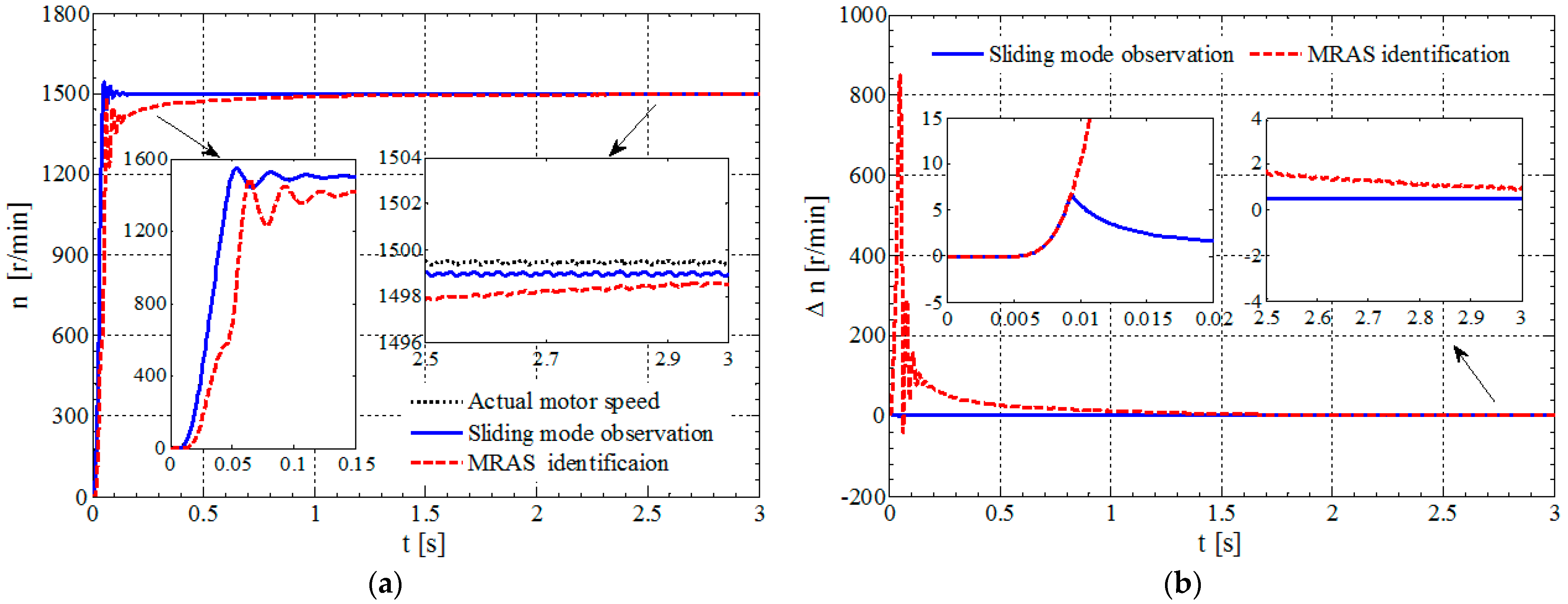
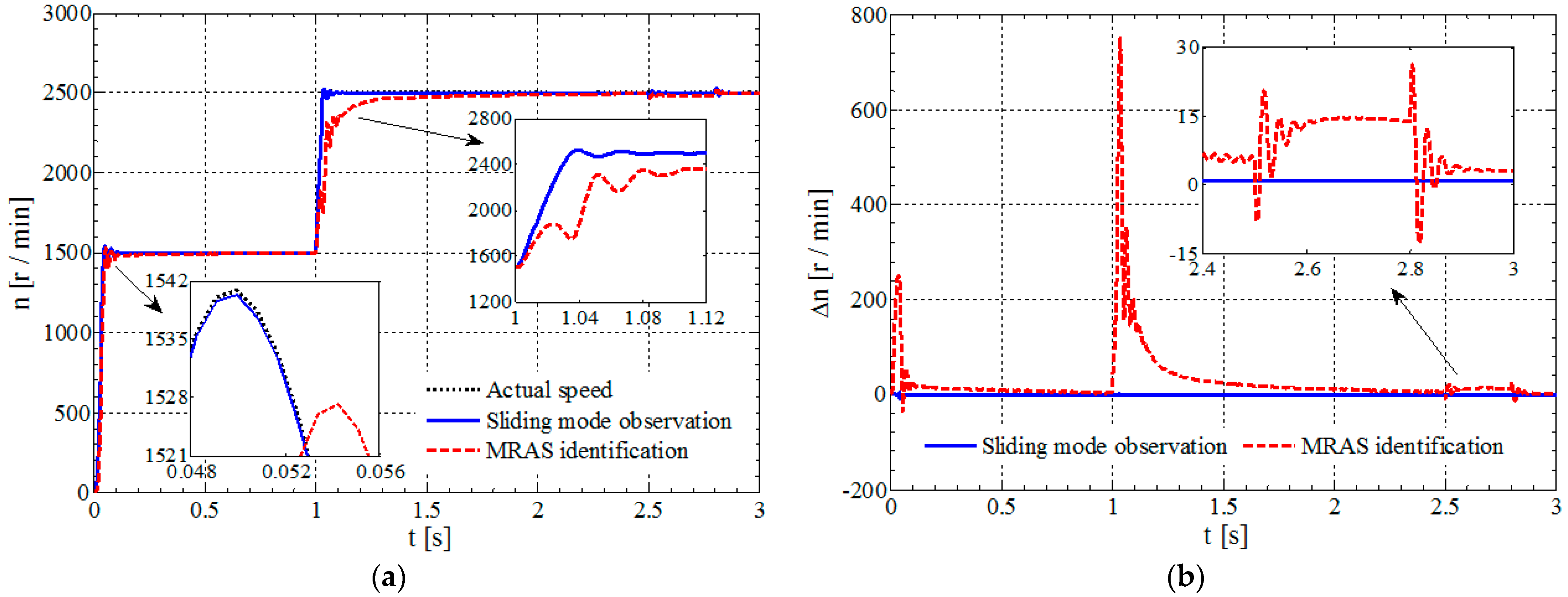
During the no-load start-up of a BL-IM, if the MRAS speed identification method is used, the observed speed reaches its peak value at 0.07 s, its rising speed is lower than the actual starting speed, the maximum dynamic tracking error is about 800 r/min; while if the proposed motor speed SMO method is used, the observed motor speed basically change synchronously with the actual motor speed, it reaches the peak value at 0.05 s, and the maximum dynamic tracking error is about 6 r/min. Therefore, compared with the MRAS speed identification method, the proposed motor speed SMO method can track the actual motor speed in a more timely manner at the moment of no-load starting, and obtain higher real-time observation performance and dynamic tracking performance.

(2)

After the BL-IM system starts with no load and enters into steady state, if the MRAS speed identification method is used, the steady-state observation error is about 1.5 r/min; while if the motor speed SMO method is used, the steady-state observation error is about 0.5 r/min. Therefore, compared with the MRAS Speed identification method, the proposed motor speed SMO method can obviously improve the steady-state observation accuracy.

The speed MRAS identification method based on rotor flux-linkage has low identification accuracy because of the pure integration link in the reference model. The observation accuracy of motor speed is inevitably affected by the cumulative error and the initial value of the pure integrator, especially at a lower speed. If the proposed motor speed SMO method is used, the shortcomings of the MRAS speed observation method can be effectively overcome and better observation performance can be obtained. In particular, the chattering phenomenon of the sliding mode observer can be overcome by replacing the traditional switching function with a smooth and continuous saturation function.

As for a BL-IM system adopting the proposed motor speed SMO method, so as to verify the speed observation performance and DDC performance under load and without speed sensor, the given signals of several controlled variables are changed at different moments. At 1.0 s, the given motor speed ω* is increased to 2500 r/min; at 2.5 s, a 8.4 n.m load torque is added, and then unloaded at 2.8 s; the given displacement α* is changed to −0.05 mm at 1.5 s, and then returned to 0.0 mm at 1.8 s; the given displacement β* is changed to 0.05 mm at 2.0 s, and then returned to 0.0 mm at 2.3 s. Figure 5, Figure 6, Figure 7, Figure 8 and Figure 9 present the observation response of motor speed, and those of rotor flux-linkage and stator current. The response of radial displacement components are given in Figure 10.

Under the conditions of loading and speed regulation, the observation response waveform and observation error waveform of motor speed are given in Figure 5. According to Figure 5, and combining Figure 4, there are the following research results:

(1) Regardless of the process of starting or speed regulation, the speed SMO method can obtain higher observation performance than the MRAS speed identification method, and can track the actual motor speed more quickly.

(2) In the process of sudden loading and unloading, when the MRAS speed identification method is adopted, obvious speed fluctuation about 25 r/min occurs; when the speed SMO method is adopted, because of its fast tracking performance and the better DDC performance of a BL-IM inverse system, the motor speed is hardly affected by the change of load.

(3) In view of the stronger real-time observation and dynamic tracking performance of the proposed speed SMO method, the BL-IM system can obtain stronger load disturbance resistance and higher steady-state speed control accuracy.

Under the conditions of loading and speed regulation, Figure 6 gives the observation response waveforms of α- and β-axis rotor flux-linkage components, Figure 7 gives the error response between the given- and observed-value of rotor flux-linkage.

According to Figure 6 and Figure 7, the following research results can be obtained:

(1)

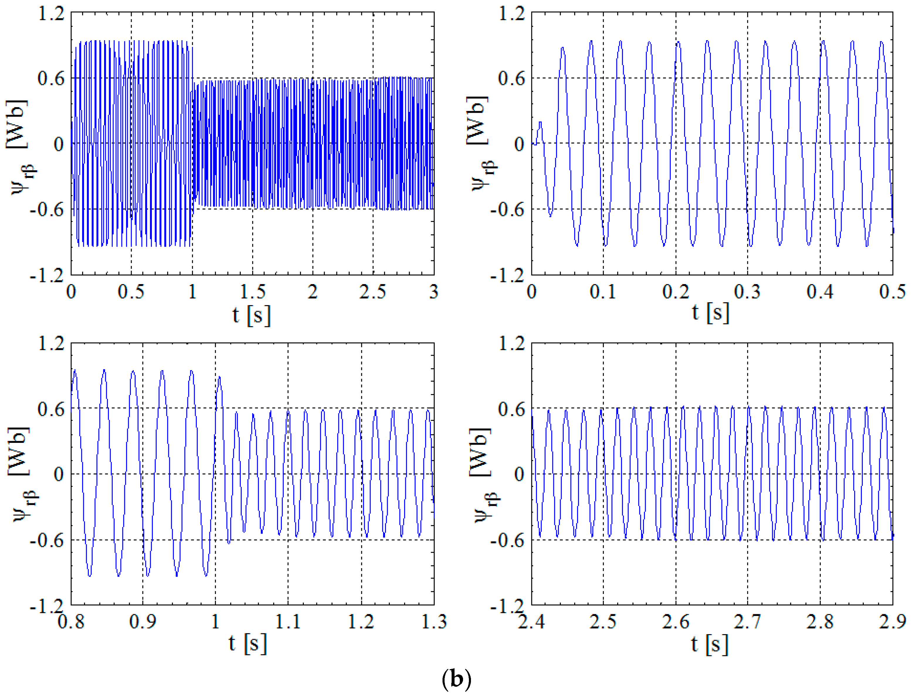
At the sudden change moment of motor speed, a transient rotor flux-linkage observation error of about 0.3 Wb appears. At the moment of load sudden change, the rotor flux-linkage fluctuation with an amplitude of 0.04 Wb appears. However, under the action of the BL-IM inverse DDC system, the transient observation error is quickly suppressed and reduced to near zero.

(2)

In steady state, the observation error of rotor flux-linkage is always kept within 0.02 Wb (i.e., within the steady-state error range of about ±2.1%). The high observation accuracy of rotor flux-linkage ensures the stable suspension operation of a BL-IM system.

In the α-β coordinate system, Figure 8 gives the observation response waveform and observation error waveform of α-axis stator current component; Figure 9 gives the observation response and observation error waveform of β-axis current component.

From Figure 8 and Figure 9, the following research results can be obtained:

(1)

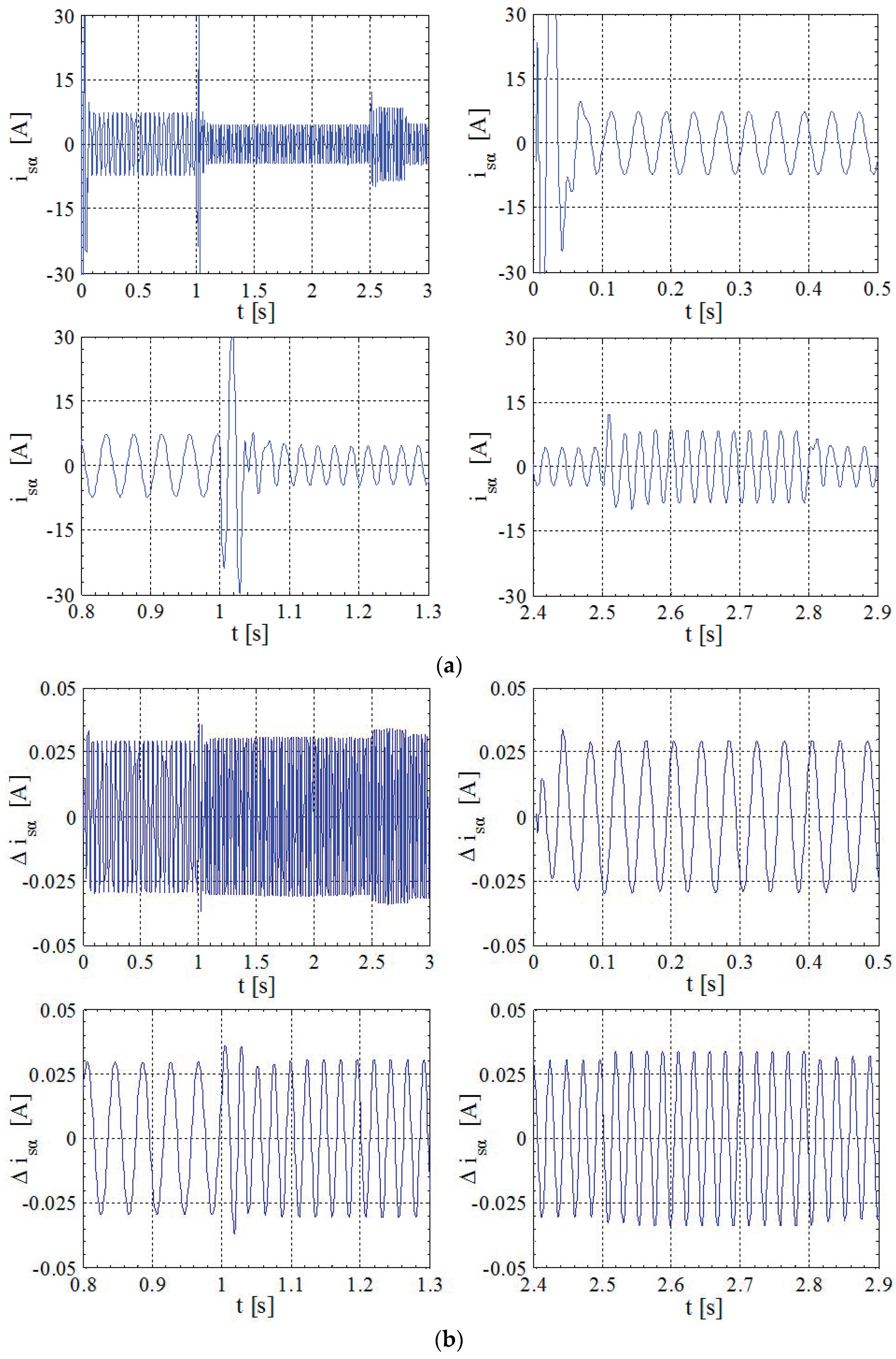
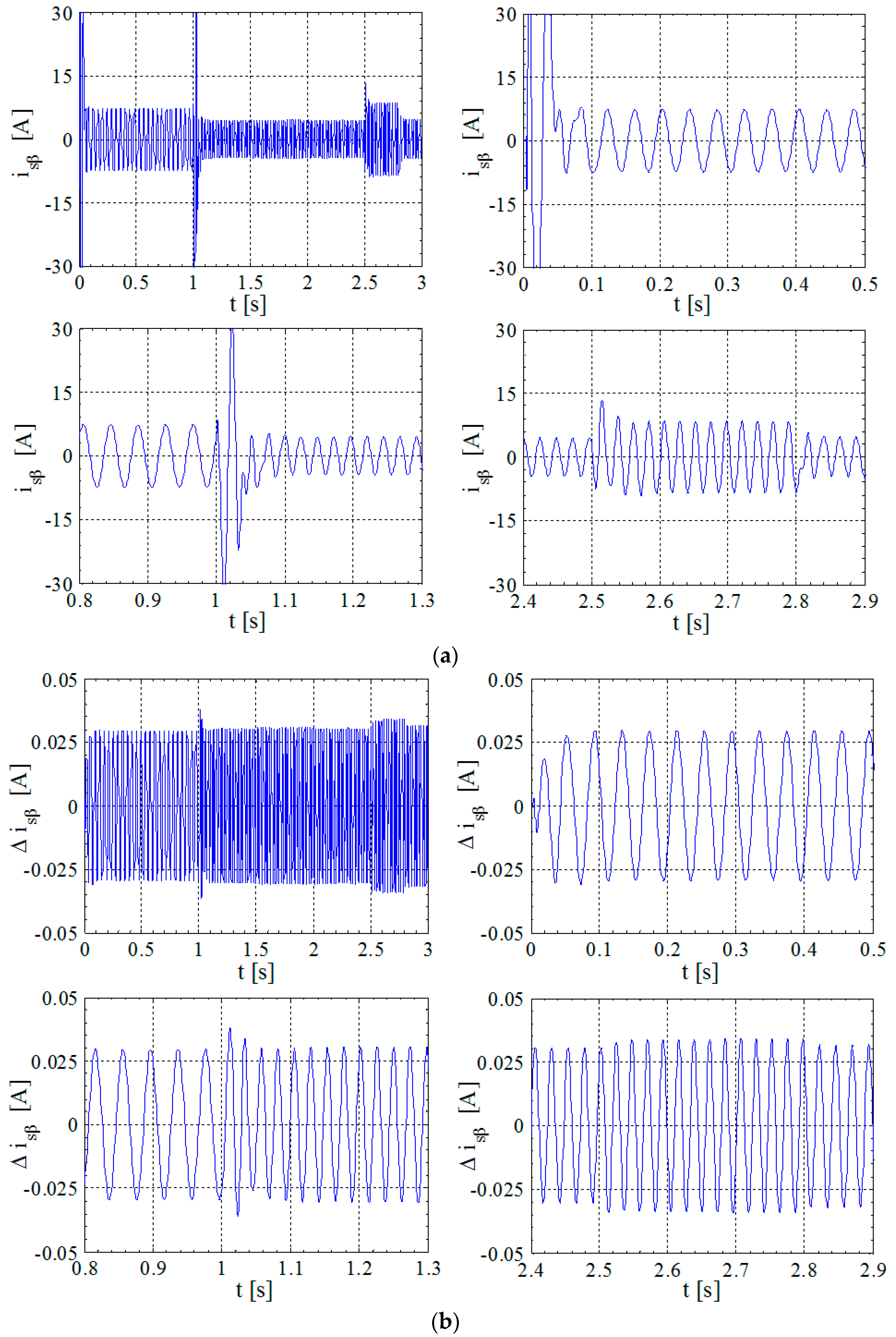
Regardless of the process of motor starting or that of speed regulation, the stator current error is always within 0.03 A.

(2)

The high-precision observation of stator current and rotor flux-linkage provides a guarantee for the high-precision sliding mode observation of motor speed, and also shows the reliability of the proposed SMO method.

The response waveforms of α- and β-axis displacements are given in Figure 10a,b; except for the artificial change process of radial displacement, the α- and β-axis displacements are always kept near zero value, and the magnetic suspension operation control of the bearingless rotor with high accuracy is obtained.

From Figure 5, Figure 6, Figure 7, Figure 8, Figure 9 and Figure 10, the following results can be obtained:

(1)

Under the speed sensorless conditions, when the motor speed suddenly changes, the stator current of the torque system can respond immediately to produce the required electromagnetic torque; the rotor flux-linkage subsystem only produces about 0.3 wb fluctuation, which is suppressed instantaneously; the displacement components are basically not affected.

(2)

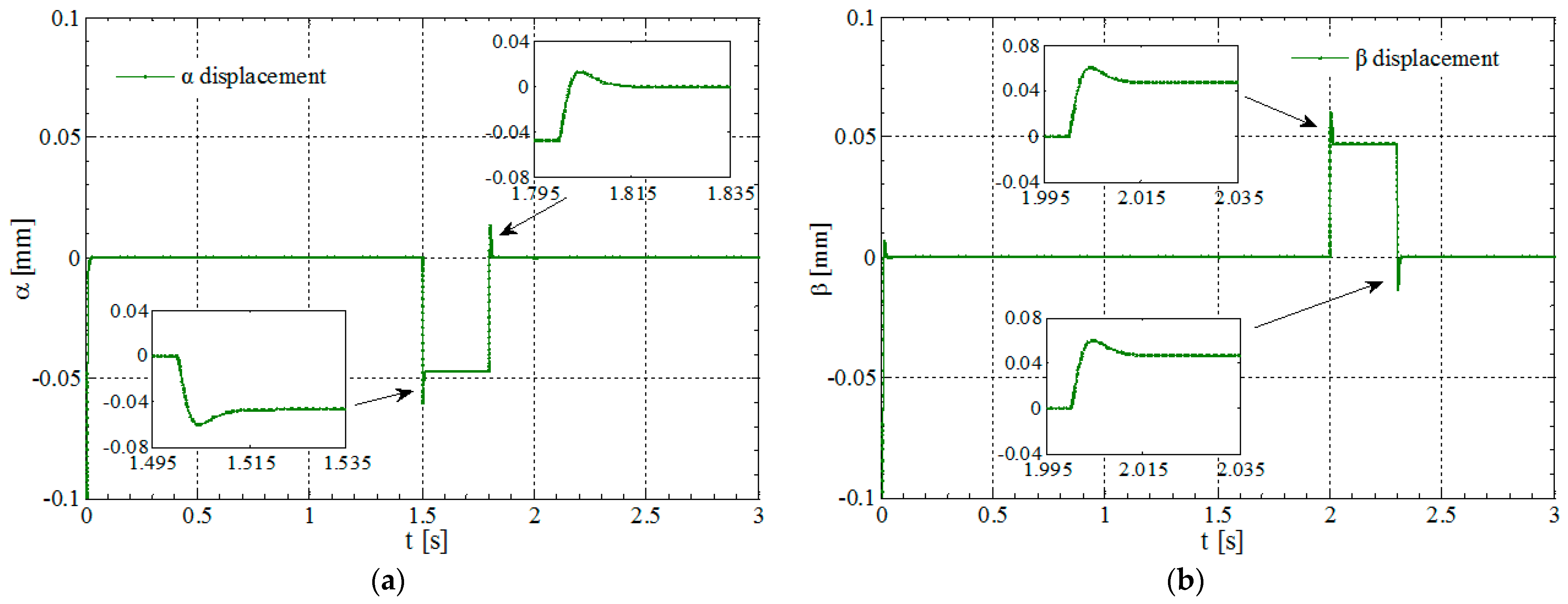
Under the speed sensorless conditions, when any one of the two radial displacement components changes suddenly, the stator current, rotor flux-linkage, and motor speed of the torque system are basically not affected. At the same time, there is no coupling phenomena between the two displacement components.

(3)

After the speed sensor is displaced by the speed sliding mode observer and the observed motor speed, rotor flux-linkage is used in the BL-IM’s inverse DDC system. The BL-IM system not only achieves stable magnetic suspension operation, but also achieves almost the same DDC performance as when the speed sensor is used [25,28]. That is to say, the speed sensorless vector control can be achieved when the proposed speed SMO method is applied to a BL-IM system.

5. Conclusions

The BL-IM is taken as a research object, and an SMO method of motor speed and rotor flux-linkage is researched. First, according to the characteristics of the BL-IM system model, the observation models of stator current and rotor flux-linkage are derived. The sign function in the observation model is displaced by a continuous saturation function, so as to eliminate or suppress the chattering problem of the sliding mode observer. Then, the SMO model of motor speed is derived, and the stability of the proposed SMO method is confirmed by Lyapunov theory. Finally, the observed motor speed and rotor flux-linkage are applied to the inverse DDC system of a BL-IM. According to the simulation results, the research conclusions are obtained as follows:

(1)

Compared with the MRAS speed identification method, whether in the process of no-load starting, or in that of load mutation and speed regulation, the proposed SMO method can realize the real-time observation or dynamic tracking of motor speed in a more timely manner and more accurately, and can effectively reduce the observation error of steady-state motor speed and improve the steady-state observation accuracy of motor speed.

(2)

On the basis of the inverse DDC system of a BL-IM and the proposed motor speed SMO method, when the observed motor speed and rotor flux-linkage are used as the feedback signals of corresponding closed loops, the stable magnetic suspension operation can be realized, and the good DDC performance between motor speed, rotor flux-linkage, and two radial displacement components can be achieved.

(3)

The proposed sliding mode observer is effective and feasible, and can be used to replace the speed sensor in a BL-IM system to achieve the stable speed sensorless magnetic suspension operation with high performance.

As for the speed SMO method of a BL-IM proposed in this paper, the speed information is not needed in the observation of rotor flux-linkage, which can effectively avoid the observation coupling problem between rotor flux-linkage and motor speed. Therefore, in the real-time implementation process, it can effectively reduce the calculation workload and improve the convergence speed of the motor speed observer. Because the algorithm of the proposed speed SMO method is not so complex, it will not affect the real-time performance in system implementation. Therefore, this technology is more suitable for the speed sensorless control system of a BL-IM, which can be applied to large-capacity electromechanical energy storage, centrifugal equipment, high-speed motorized spindle drives, and military and aerospace industries. However, in the change process of motor speed, there is still instantaneous fluctuation of rotor flux-linkage, which needs further improvement. In addition, in order to improve the DDC performance, the speed sensorless control system of a BL-IM is constructed on the basis of inverse system decoupling. Compared with the speed observation algorithm, the inverse system decoupling algorithm is relatively complex; therefore, in order to ensure the BL-IM system’s real-time properties, the adopted microprocessor should have relatively high performance as far as possible.

References

1. Chiba, A.; Fukao, T.; Ichkawa, O.; Oshima, M.; Takemoto, M.; Dorrell, D.G. Magnetic Bearings and Bearingless Drives; Newnes: Tokyo, Japan, 2005. [Google Scholar]
2. Wang, X.; Zhang, Y.; Gao, P. Design and Analysis of Second-Order Sliding Mode Controller for Active Magnetic Bearing. Energies 2020, 13, 5965. [Google Scholar] [CrossRef]
3. Cheng, X.; Cheng, B.-X.; Deng, S.; Zhou, R.-G.; Lu, M.-Q.; Wang, B. State-feedback decoupling control of 5-DOF magnetic bearings based on α-order inverse system. Mechatronics 2020, 68, 102358. [Google Scholar] [CrossRef]
4. Murakami, I.; Mori, H.; Shimizu, M.; Quan, N.M.; Ando, Y. Study on rigidity of the superconducting magnetic bearing. Int. J. Appl. Electromagn. Mech. 2019, 59, 191–200. [Google Scholar] [CrossRef]
5. Sun, X.; Su, B.; Chen, L.; Yang, Z.; Xu, X.; Shi, Z. Precise control of a four degree-of-freedom permanent magnet biased active magnetic bearing system in a magnetically suspended direct-driven spindle using neural network inverse scheme. Mech. Syst. Signal Process. 2017, 88, 36–48. [Google Scholar] [CrossRef] [Green Version]
6. Yang, Z.; Wan, L.; Sun, X.; Li, F.; Chen, L. Sliding Mode Variable Structure Control of a Bearingless Induction Motor Based on a Novel Reaching Law. Energies 2016, 9, 452. [Google Scholar] [CrossRef] [Green Version]
7. Chiba, A.; Furuichi, R.; Aikawa, Y.; Shimada, K.; Takamoto, Y.; Fukao, T. Stable Operation of Induction-Type Bearingless Motors Under Loaded Conditions. IEEE Trans. Ind. Appl. 1997, 33, 919–924. [Google Scholar] [CrossRef]
8. Bu, W.S.; Li, Z.Y. LS-SVM Inverse System Decoupling Control Strategy of Bearingless Induction Motor Considering Stator Cur-rent Dynamics. IEEE Access 2019, 7, 132130–132139. [Google Scholar] [CrossRef]
9. Hiromi, T.; Katou, T.; Chiba, A.; Rahman, M.A.; Fukao, T. A Novel Magnetic Suspension-Force Compensation in Bearingless Induction-Motor Drive with Squirrel-Cage Rotor. IEEE Trans. Ind. Appl. 2007, 43, 66–76. [Google Scholar] [CrossRef]
10. Zhu, Z.; Zhu, J.; Guo, X.; Jiang, Y.; Sun, Y. Numerical Modeling of Suspension Force for Bearingless Flywheel Machine Based on Differential Evolution Extreme Learning Machine. Energies 2019, 12, 4470. [Google Scholar] [CrossRef] [Green Version]
11. Sun, X.; Jin, Z.; Wang, S.; Yang, Z.; Li, K.; Fan, Y.; Chen, L. Performance improvement of torque and suspension force for a novel five-phase BFSPM machine for flywheel energy storage systems. IEEE Trans. Appl. Supercond. 2019, 29, 1–4. [Google Scholar] [CrossRef]
12. Bu, W.; Zhang, X.; Qiao, Y.; Li, Z.; Zhang, H. Equivalent two-phase mutual inductance model and measurement algorithm of three-phase bearingless motor. Trans. Inst. Meas. Control. 2016, 40, 630–639. [Google Scholar] [CrossRef]
13. Yang, Z.; Ji, J.; Sun, X.; Zhu, H.; Zhao, Q. Active Disturbance Rejection Control for Bearingless Induction Motor Based on hyperbolic tangent tracking differentiator. IEEE J. Emerg. Sel. Top. Power Electron. 2020, 8, 2623–2633. [Google Scholar] [CrossRef]
14. Sun, X.; Shi, Z.; Chen, L.; Yang, Z. Internal Model Control for a Bearingless Permanent Magnet Synchronous Motor Based on Inverse System Method. IEEE Trans. Energy Convers. 2016, 31, 1539–1548. [Google Scholar] [CrossRef]
15. Bu, W.; Tu, X.; Lu, C.; Pu, Y. Adaptive feedforward vibration compensation control strategy of bearingless induction motor. Int. J. Appl. Electromagn. Mech. 2020, 63, 199–215. [Google Scholar] [CrossRef]
16. Sun, X.; Su, B.; Wang, S.; Yang, Z.; Lei, G.; Zhu, J.; Guo, Y. Performance Analysis of Suspension Force and Torque in an IBPMSM with V-Shaped PMs for Flywheel Batteries. IEEE Trans. Magn. 2018, 54, 1–4. [Google Scholar] [CrossRef]
17. Yang, Z.; Wan, L.; Sun, X.; Chen, L.; Chen, Z. Sliding Mode Control for Bearingless Induction Motor Based on a Novel Load Torque Observer. J. Sens. 2016, 2016, 1–10. [Google Scholar] [CrossRef] [Green Version]
18. Wu, X.; Yang, Y.; Liu, Z. Theoretical analysis and simulation of single-winding bearingless switched reluctance generator with wider rotor teeth. Int. J. Appl. Electromagn. Mech. 2018, 56, 387–398. [Google Scholar] [CrossRef]
19. Bu, W.; He, F.; Li, Z.; Zhang, H.; Shi, J. Neural Network Inverse System Decoupling Control Strategy of BLIM Considering Stator Current dynamics. Trans. Inst. Meas. Control 2019, 41, 621–630. [Google Scholar] [CrossRef]
20. Yang, Z.; Ding, Q.; Sun, X.; Ji, J.; Zhao, Q. Design and analysis of a novel wound rotor for a bearingless induction motor. Int. J. Electron. 2019, 106, 1829–1844. [Google Scholar] [CrossRef]
21. Sun, X.; Chen, L.; Jiang, H.; Yang, Z.; Chen, J.; Zhang, W. High-Performance Control for a Bearingless Permanent-Magnet Synchronous Motor Using Neural Network Inverse Scheme Plus Internal Model Controllers. IEEE Trans. Ind. Electron. 2016, 63, 3479–3488. [Google Scholar] [CrossRef]
22. Wang, H.; Li, F. Design Consideration and Characteristic Investigation of Modular Permanent Magnet Bearingless Switched Reluctance Motor. IEEE Trans. Ind. Electron. 2019, 67, 4326–4337. [Google Scholar] [CrossRef]
23. Bu, W.; Chen, Y.; Zu, C. Stator flux orientation inverse system decoupling control strategy of bearingless induction motor considering stator current dynamics. IEEJ Trans. Electr. Electron. Eng. 2019, 14, 640–647. [Google Scholar] [CrossRef]
24. Sun, Y.; Tang, J.; Xu, P. Design of a Bearingless Outer Rotor Induction Motor. Energies 2017, 10, 705. [Google Scholar] [CrossRef] [Green Version]
25. Bu, W.; Zhang, X.; He, F. Sliding mode variable structure control strategy of bearingless induction motor based on inverse system decoupling. IEEJ Trans. Electr. Electron. Eng. 2018, 13, 1052–1059. [Google Scholar] [CrossRef]
26. Yang, Z.; Chen, X.; Sun, X.; Bao, C.; Lu, J. Rotor radial disturbance control for a bearingless induction motor based on improved active disturbance rejection control. COMPEL Int. J. Comput. Math. Electr. Electron. Eng. 2019, 38, 138–152. [Google Scholar] [CrossRef]
27. Ye, X.; Yang, Z.; Zhang, T. Modelling and performance analysis on a bearingless fixed-pole rotor induction motor. IET Electr. Power Appl. 2019, 13, 251–258. [Google Scholar] [CrossRef]
28. Bu, W.; Li, B.; He, F.; Li, J. Inverse system decoupling sliding mode control strategy of bearingless induction motor considering current dynamics. Int. J. Appl. Electromagn. Mech. 2019, 60, 63–78. [Google Scholar] [CrossRef]
29. Beck, M.; Naunin, D. A new method for the calculation of the slip frequency for a sensorless speed control of a squirrel-cage induction motor. In Proceedings of the IEEE Power Electronics Specialists Conference, Toulouse, France, 24–28 June 1985; pp. 678–683. [Google Scholar]
30. Zhong, Z.F.; Jin, M.J.; Shen, J.X. Full Speed Range Sensorless Control of Permanent Magnet Synchronous Motor with Phased PI Regulator-Based Model Reference Adaptive System. Proc. Chin. Soc. Electr. Eng. 2018, 38, 1203–1211. [Google Scholar]
31. Yildiz, R.; Barut, M.; Zerdali, E. A Comprehensive Comparison of Extended and Unscented Kalman Filters for Speed-Sensorless Control Applications of Induction Motors. IEEE Trans. Ind. Inform. 2020, 16, 6423–6432. [Google Scholar] [CrossRef]
32. Orlowska-Kowalska, T.; Korzonek, M.; Tarchala, G. Stability Improvement Methods of the Adaptive Full-Order Observer for Sensorless Induction Motor Drive—Comparative Study. IEEE Trans. Ind. Inform. 2019, 15, 6114–6126. [Google Scholar] [CrossRef]
33. Qin, F.; He, Y.-K.; Liu, Y.; Zhang, W. Comparative investigation of sensorless control with two high-frequency signal injection schemes. Proc. Chin. Soc. Electr. Eng. 2005, 25, 116–121. [Google Scholar]
34. Shi, H.-Y.; Feng, Y. High-order Terminal Sliding Mode Flux Observer for Induction Motors. Acta Autom. Sin. 2012, 38, 288–294. [Google Scholar] [CrossRef]
35. Sun, Y.X.; Tang, J.W.; Shi, K.; Zhu, H.Q. Vector control of speed sensorless bearingless induction motors using improved MRAS. Control Theory Appl. 2019, 36, 939–950. [Google Scholar]
36. Yang, Z.; Wang, M.; Sun, X. Speed-sensorless vector control system of bearingless induction motor based on reactive power MRAS of torque winding. J. Sichuan Univ. Eng. Sci. Ed. 2014, 46, 140–146. [Google Scholar]
37. Yang, Z.; Fan, R.; Sun, X.; Dong, D.; Zhu, H. Speed-sensorless control system of bearingless induction motor based on the extended Kalman filter. Chin. J. Sci. Instrum. 2015, 36, 1023–1030. [Google Scholar] [CrossRef]
38. Sun, Y.; Shen, Q.; Shi, K.; Zhu, K. Speed-Sensorless Control System of Bearingless Induction Motor Based on the Novel Extended Kalman Filter. Trans. China Electrotech. Soc. 2018, 33, 2946–2955. [Google Scholar]
39. Zhao, Q.; Yang, Z.; Sun, X.; Ding, Q. Speed-sensorless control system of a bearingless induction motor based on iterative central difference Kalman filter. Int. J. Electron. 2020, 107, 1524–1542. [Google Scholar] [CrossRef]
40. Yang, Z.; Li, F.; Chen, Z.; Sun, X. Revolving speed self-detecting control based on low-frequency signal injection for bearingless induction motor. Trans. Chin. Soc. Agric. Eng. 2017, 33, 41–47. [Google Scholar]
41. Sun, X.; Chen, L.; Yang, Z.; Zhu, H. Speed-Sensorless Vector Control of a Bearingless Induction Motor with Artificial Neural Network Inverse Speed Observer. IEEE/ASME Trans. Mechatron. 2013, 18, 1357–1366. [Google Scholar] [CrossRef]
42. Cheng, S.; Jiang, H.; Huang, J.; Kang, M. Position sensorless control based on sliding mode observer for multiphase bearingless motor with single set of windings. Trans. China Electrotech. Soc. 2012, 27, 71–77. [Google Scholar]
Figure 1. Suspension force generation schematic diagram.
Energies 14 00864 g001
Figure 2. Schematic diagram of speed sliding mode observer.
Energies 14 00864 g002
Figure 3. Schematic diagram of a bearingless induction motor (BL-IM) speed sensorless control system.
Energies 14 00864 g003
Figure 4. Speed response waveform during no-load start-up: (a) Observed motor speed; (b) Observation error of motor speed.
Energies 14 00864 g004
Figure 5. Speed response waveform with load: (a) Observed motor speed; (b) Observation error of motor speed.
Energies 14 00864 g005
Figure 6. Response of rotor flux linkage: (a) α-axis rotor flux-linkage; (b) β-axis rotor flux-linkage.
Energies 14 00864 g006aEnergies 14 00864 g006b
Figure 7. Observation error response of rotor flux-linkage.
Energies 14 00864 g007
Figure 8. Observation response of α-axis stator current: (a) Observed α-axis current; (b) Observation error of α-axis current.
Energies 14 00864 g008
Figure 9. Observation response of β-axis stator current: (a) Observed β-axis current; (b) Observation error of β-axis current.
Energies 14 00864 g009
Figure 10. Displacement response waveforms: (a) α displacement component; (b) β displacement component.
Energies 14 00864 g010