Improving PV Resilience by Dynamic Reconfiguration in Distribution Grids: Problem Complexity and Computation Requirements

Abstract

The dissemination of low-carbon technologies, such as urban photovoltaic distributed generation, imposes new challenges to the operation of distribution grids. Distributed generation may introduce significant net-load asymmetries between feeders in the course of the day, resulting in higher losses. The dynamic reconfiguration of the grid could mitigate daily losses and be used to minimize or defer the need for network reinforcement. Yet, dynamic reconfiguration has to be carried out in near real-time in order to make use of the most updated load and generation forecast, this way maximizing operational benefits. Given the need to quickly find and update reconfiguration decisions, the computational complexity of the underlying optimal scheduling problem is studied in this paper. The problem is formulated and the impact of sub-optimal solutions is illustrated using a real medium-voltage distribution grid operated under a heavy generation scenario. The complexity of the scheduling problem is discussed to conclude that its optimal solution is infeasible in practical terms if relying upon classical computing. Quantum computing is finally proposed as a way to handle this kind of problem in the future.

1. Introduction

New preventive grid control paradigms that make use of information on disaggregated net-load forecasts to estimate operational problems and anticipate potential opportunities to improve such operation have recently attracted considerable attention from the electric power industry. The new preventive capabilities of such control paradigms unleash flexibility from the grid side, adding such flexibility to the demand side flexibility available through load and generation responsive services [1]. Among such preventive control capabilities, dynamic reconfiguration appears as a new automation technology capable of both mitigating congestion and improving efficiency in networks operated under high levels of renewables [2]. Such potential is quite easy to recognize when generation resources are photovoltaic (PV) [3]. Yet, the challenges involved in optimal control for dynamic reconfiguration are not minor, and many opportunities lie ahead for those who will be able to tackle its full complexity.

In general, urban PV generation profiles do not match the load profiles of distribution grids, both in temporal and in spatial terms, resulting in time and space asymmetries on the network net load during the course of the day. As PV generation gets heavier over the long term, these asymmetries will pose a new challenge to the operation of distribution grids as they result in increased network losses and, at the limit, line current magnitude overloads may happen.

Using network optimization algorithms [4], the grid can be reconfigured such that it dynamically adapts to its real-time net load profile [5]. The goal of the optimization problem is to minimize network losses on the day-ahead period, given a starting network configuration. Ideally, the optimal network reconfiguration would not have any time constraints to undertake its switching operations (i.e., it would be immediately effective as a response to a change in the load) and it would not have any limitation on the number of switching operations when (instantly) changing from the current network configuration to the next one. Thus, the network reconfiguration on a given time would be completely independent from the previous network configuration, resulting on a simpler optimization problem. Additionally, as the problem would be independent of future network configurations, there would be no need to take into account load and PV generation forecast.

In real networks there are, however, constraints both on reconfiguration time and completeness. Several factors contribute to the reconfiguration latency: delay on real-time data collection of network load and PV generation; computation time taken to find an optimal reconfiguration for the net load data; time taken to execute the network switching operations. On the other hand, the number of switching operations is limited by the cost of each operation in terms of switching equipment wearing and by the operational risk on the network of each switching operation [6]. This limitation makes the reconfiguration problem much more demanding in computational terms, since one has to find a limited schedule of operations to be made over time that guarantees successive optimality stages for the network when loaded based on available forecast. It is important to understand how the computational complexity scales, since the computation time taken to find the reconfiguration schedule may have a significant impact on the reconfiguration latency. This is especially relevant when the obtained schedule contains switching operations that need to be carried out immediately after forecast availability.

Literature is rich in optimization approaches to the static version of the reconfiguration problem. The first report of such a problem for losses minimization dates back to 1975. Since then, hundreds of works have addressed different versions of the static problem, tackling different objectives and constraints with a variety of heuristic solution approaches, such as using genetic algorithms [7,8], particle swarm optimization [9] and bacteria foraging optimization [10]. A comprehensive survey of reconfiguration problems and solution approaches can be found in [11].

Dynamic reconfiguration is not so well studied as an optimization problem, often being addressed in the context of post-contingency system restoration only [12,13]. As a restoration problem, optimization objectives are usually related to re-energizing the isolated section of the grid as quickly as possible, limiting the scheduling to the sequencing of the switching operations in time [14]. Self-healing has also been addressed as a dynamic reconfiguration problem in the distribution system restoration context [15,16].

Since the full dynamic reconfiguration problem has been considered computationally intractable, the approaches found in the literature treat this problem approximately, not fully addressing its complexity. We believe that quantum computing offers the possibility of handling this problem with its full complexity, enabling the computation of the optimal solution. This paper is our first step in pursuing that goal. Its main contributions include:

• A new formulation of the optimal dynamic reconfiguration problem for losses minimization;
• A quantification of problem complexity and how this complexity scales with the number of switching operations and with the number of time steps (i.e., time span of reconfiguration schedule multiplied by time resolution);
• An illustration of the benefits of finding the optimal dynamic reconfiguration solution over a real network model;
• A discussion of the prospective use of quantum computing to address the complexity of the full dynamic reconfiguration problem in the future.

This paper is organized as follows. After this Introduction, the reconfiguration problem is mathematically formulated in Section 2. Afterwards, an illustrative example of a solution for this problem is given in Section 3. In Section 4, the time complexity of the problem is discussed and quantum computing is proposed as a means to tackle the problem in useful time. Finally, Section 5 concludes the paper.

2. Problem Formulation

Let N and A be, respectively, the set of nodes and the set of arcs of a graph G of a distribution network. For each node $n\in N$, its net load at a given time t is defined as

$$S_n\left(t\right)=S_n^{\mathrm{LOAD}}\left(t\right)+P_n^{\mathrm{PV}}\left(t\right)$$

(1)

where $S_n^{\mathrm{LOAD}}\left(t\right)$ is the consumers load aggregated on node n and $P_n^{\mathrm{PV}}\left(t\right)$ is the total PV generation injected on this node (a negative load value). This model assumes that no reactive power is injected by PV producers.

Assuming that the distribution grid is always required to operate radially, the subset $T\subseteq A$ contains all the network arcs belonging to the operational spanning tree in a given time. Thus, T completely represents a network configuration. Additionally, $T\in \mathrm{ST}\left(G\right)$ where $\mathrm{ST}\left(G\right)$ is the set of all possible spanning trees of G.

Given the net load $S\left(t\right)$ on all nodes and the network configuration T, a power-flow analysis computes the current magnitude $I_m(S\left(t\right),T)$ on the operating arcs $m\in T$. The total network active power losses at a given time are defined as

$$L(S\left(t\right),T)=\sum _{m\in T}{R}_m{I}_m^2(S\left(t\right),T)$$

(2)

where $R_m$ is the resistance of arc m.

In the following subsections several reconfiguration problems are formulated as optimization problems. To determine each problem computation time, it is important to understand how the time complexity of each problem scales. The search space of each of these problems may include the network configurations space $\mathrm{ST}\left(G\right)$ and multiple dimensions of time. We do not consider the scaling with the network size. To this end, we will formulate problem complexity as the number of individual and independent network configuration optimization runs (if the network configurations space is included in the search space of the problem) or power-flow runs (otherwise) needed to solve the problem, thus leaving the network size dependence to each network optimization or power-flow run.

2.1. Unrestricted Optimal Reconfiguration

As described in the Introduction, if there were no limitations on the number of switching operations on the network, finding the optimal network configuration $T^{*}$ on a given time would be independent of previous and future configurations. This optimization problem would be stated as the minimization of total network losses on a given time t, as defined by

$$T^{*}\left(t\right)=\underset{T\in \mathrm{ST}\left(G\right)}{arg\; min}L(S\left(t\right),T).$$

(3)

The time complexity of this problem is p configuration optimizations, where p is the number of time steps on which t is given. Thus, this problem grows linearly with the time resolution.

2.2. Optimal Static Configuration

If no switching operations are allowed during the day, the network must be operated in a single static configuration. The optimal static configuration is the one that minimizes the energy losses for the whole day, as defined by

$$T_{\mathrm{day}}^{*}=\underset{T\in \mathrm{ST}\left(G\right)}{arg\; min}{\int }_{t\in \mathrm{TI}}L(S\left(t\right),T)dt$$

(4)

where TI is the time interval considered for the optimization problem, i.e., the 24 h day period.

Since there is a single network optimization for the whole day, the time complexity of this problem is constant and equal to one configuration optimization.

2.3. Time-Bounded Linear Dynamic Reconfiguration

Let $T+x$ represent the application of switching operation x on network configuration $T\in \mathrm{ST}\left(G\right)$, and let $T^{\prime }-x$ denote the reversion of switching operation x on configuration $T^{\prime }\in \mathrm{ST}\left(G\right)$. The same notation will be used if x is replaced by the set or the sum of several switching operations. A reconfiguration schedule between the initial configuration $T^I$ and the final configuration $T^F$ contains the minimum set of switching operations O needed to transform configuration $T^I$ into configuration $T^F$, as given by

$$T^F=T^I+\sum _{x\in O}x\equiv T^I+O.$$

(5)

A schedule with the same switching operations reverted would bring configuration $T^F$ back to configuration $T^I$:

$$T^I=T^F-\sum _{x\in O}x\equiv T^F-O.$$

(6)

The set of switching operations O can also be defined as the difference between the two configurations: $O=T^F-T^I$. Although O can be immediately determined from both configurations, the same is not true for the optimal time for each switching operation. A simple approach to this problem could be to restrict (3) to configurations $T^I$, $T^F$ and all configurations in between, resulting from the application of any subset of O in $T^I$, as given by

$$T^{*}\left(t\right)=\underset{T\in \{T^I+Q:Q\in \mathcal{P}\left(O\right)\}}{arg\; min}L(S\left(t\right),T)$$

(7)

where $\mathcal{P}\left(O\right)$ denotes the power set of O, i.e., the set of all subsets of O, including the empty set and O itself. It is important to note that $\left|\mathcal{P}\left(O\right)\right|=2^{\left|\right(O\left)\right|}$, which means that the search space on every time point grows exponentially with the number of differences between $T^I$ and $T^F$. Although this approach restricts the schedule to a path between $T^I$ and $T^F$, it does not limit the number of switching operations since the path can be traversed backwards and forward as $S\left(t\right)$ changes over time.

To ensure that the path between $T^I$ and $T^F$ is always traversed forward, a single time point $\mathrm{inst}\left(x\right)\in \mathrm{TI}$ is assigned to each switching operation $x\in O$, where TI is the maximum time interval for the schedule. Formally, O can be represented as an arbitrarily-ordered sequence of $O_k$ elements, where $k=1,...,\left|O\right|$. The time points for all switching operations $O_k$ can also be represented as a sequence with the same ordering: ${\mathrm{inst}}_k=\mathrm{inst}\left(O_k\right)$. The sequence pair $(O,\mathrm{inst})$ completely defines a schedule. The optimal value for the switching operations time is then given by

$${\mathrm{inst}}^{*}(T^I,O)=\underset{\mathrm{inst}\in {\mathrm{TI}}^{\left|O\right|}}{arg\; min}{\int }_{t\in \mathrm{TI}}L\left[S\left(t\right),\mathrm{conf}(T^I,O,\mathrm{inst},t)\right]dt$$

(8)

where $\mathrm{conf}(T^I,O,\mathrm{inst},t)$ is the network configuration at time t with a schedule $(O,\mathrm{inst})$ starting at configuration $T^I$, as defined by

$$\mathrm{conf}(T^I,O,\mathrm{inst},t)\equiv T^I+\sum _{k=1}^{\left|O\right|}\left\{\begin{array}{cc}{O}_k\hfill & {\mathrm{inst}}_k<t\hfill \\ \varnothing \hfill & \mathrm{otherwise}\hfill \end{array}\right..$$

(9)

Note that the optimal schedule may not include all switching operations of O. The discarded operations $O_k$ will have their time points assigned to the end of TI: ${\mathrm{inst}}_k=sup\left(\mathrm{TI}\right)$.

Since the set of switching operations to perform is already known, the search space for this problem does not include the network configurations space $\mathrm{ST}\left(G\right)$. Thus, the time complexity of this problem cannot be expressed as the number of network configuration optimizations since no such optimization is made here. Instead, we express time complexity for this problem as the number of power-flow computations, i.e., the number of computations of $L\left[S\left(t\right),\mathrm{conf}\right]$. Let p be the number of time steps within the maximum time interval TI. Then, the search space ${\mathrm{TI}}^{\left|O\right|}$ is discretized into $p^{\left|O\right|}$ points and the integral on (8) becomes the summation of p computations of L. The time complexity for this problem is then $p^{\left|O\right|}p=p^{\left|O\right|+1}$ power-flow computations.

The goal of a daily reconfiguration schedule is to always return, at a given time of the day, to the same configuration (say, configuration $T^I$) everyday. Thus, the daily schedule path is cyclic but not necessarily the same every day since $S\left(t\right)$ changes from one day to the other. On a cyclic schedule between configurations $T^I$ and $T^F$, if we also impose that configuration $T^F$ occurs at another given time of the day, then this schedule can be converted into two linear time-bounded schedules from $T^I$ to $T^F$ and from $T^F$ to $T^I$ (reverting the switching operations on O) and solved by (8) as two independent problems.

2.4. Time-Unbounded Cyclic Dynamic Reconfiguration

The restriction of having configuration $T^I$ everyday at the same given time is necessary to have a cyclic schedule, as we are interested in finding a daily schedule. Adding the same restriction for configuration $T^F$ could severely constrain the problem, degrading the optimality from the obtained schedule. Thus, we are interested in finding an optimal schedule which does not impose any time constraint on configuration $T^F$.

This problem can be formulated as the linear time-bounded problem of (8) but with two important differences: the time interval for the schedule (TI) is now defined as a complete 24 h period between the given configuration $T^I$ time from two consecutive days, thus giving the time-unbounded nature; and each switching operation $O_k$ now has two time points—one to apply the operation (${\mathrm{inst}}_k^{+}$) and the other to revert it (${\mathrm{inst}}_k^{-}$), giving the cyclic nature.

A constraint must be added to ensure that any reverted operation always occurs after the original one: ${\mathrm{inst}}_k^{+}<{\mathrm{inst}}_k^{-}$, ${\forall }_{k=1,...,\left|O\right|}$. The special case ${\mathrm{inst}}_k^{+}={\mathrm{inst}}_k^{-}=0$ is allowed to indicate that the operation $O_k$ was discarded from the optimal schedule (and thus configuration $T^F$ is never reached in the schedule). Note that, even if all switching operations in O are included in the schedule, configuration $T^F$ is only reached if all these operations are active at some time of the schedule.

The sequence triplet $(O,{\mathrm{inst}}^{+},{\mathrm{inst}}^{-})$ now defines the schedule. The optimal schedule time points are given by -4.6cm 0cm

$${({\mathrm{inst}}^{+},{\mathrm{inst}}^{-})}^{*}(T^I,O)=\underset{\begin{array}{c}{\mathrm{inst}}^{+}\in {\mathrm{TI}}^{\left|O\right|}\\ {\mathrm{inst}}^{-}\in {\mathrm{TI}}^{\left|O\right|}\\ {\mathrm{inst}}_k^{+}<{\mathrm{inst}}_k^{-}\bigvee {\mathrm{inst}}_k^{+}={\mathrm{inst}}_k^{-}=0,{\forall }_k\end{array}}{arg\; min}{\int }_{t\in \mathrm{TI}}L\left[S\left(t\right),\mathrm{conf}(T^I,O,{\mathrm{inst}}^{+},{\mathrm{inst}}^{-},t)\right]dt$$

(10)

where $\mathrm{conf}(T^I,O,{\mathrm{inst}}^{+},{\mathrm{inst}}^{-},t)$ is now defined as

$$\mathrm{conf}(T^I,O,{\mathrm{inst}}^{+},{\mathrm{inst}}^{-},t)\equiv T^I+\sum _{k=1}^{\left|O\right|}\left\{\begin{array}{cc}{O}_k\hfill & {\mathrm{inst}}_k^{+}<t<{\mathrm{inst}}_k^{-}\hfill \\ \varnothing \hfill & \mathrm{otherwise}\hfill \end{array}\right..$$

(11)

As on the previous problem, the search space does not include the network configurations space given that the set of switching operations is already known, so the problem time complexity is given as the number of power-flow computations. Let p be the number of time steps within the maximum time interval TI. Then, the time complexity for this problem is $p{\left(1+\frac{p(p-1)}{2}\right)}^{\left|O\right|}$ power-flow computations.

2.5. Open Cyclic Dynamic Reconfiguration

In the previous dynamic reconfiguration problems, both configurations $T^I$ and $T^F=T^I+O$ had to be provided. As pointed out on previous section, configuration $T^I$ and its time must be given in order to obtain a cyclic schedule. This configuration can be obtained as the optimal configuration on its given time. The purpose of configuration $T^F$ was to impose a limit in the number of switching operations on a cyclic schedule, starting from configuration $T^I$. As with configuration $T^I$, configuration $T^F$ can be obtained as the optimal configuration on some given time. In general, the number of differences between both configurations is larger than the number of allowed switching operations per day. Then, to limit the number of differences, only the most beneficial operations of $T^F$ in terms of losses reduction on its fixed time are considered. Both actions of fixing a time to optimize configuration $T^F$ and truncating the configuration may degrade the optimality of the schedule.

It is possible to obtain an optimal schedule ${(O,{\mathrm{inst}}^{+},{\mathrm{inst}}^{-})}^{*}$ without providing a configuration $T^F$. Instead, it is enough to give the maximum number of daily switching operations, m, along with configuration $T^I$, as given by -4.6cm 0cm

$${(O,{\mathrm{inst}}^{+},{\mathrm{inst}}^{-})}^{*}(T^I,m)=\underset{\begin{array}{c}O\in \{T^F-T^I:T^F\in \mathrm{ST}\left(G\right)\}\\ {\mathrm{inst}}^{+}\in {\mathrm{TI}}^m\\ {\mathrm{inst}}^{-}\in {\mathrm{TI}}^m\\ \left|O\right|=m\\ {\mathrm{inst}}_k^{+}<{\mathrm{inst}}_k^{-}\bigvee {\mathrm{inst}}_k^{+}={\mathrm{inst}}_k^{-}=0,{\forall }_k\end{array}}{arg\; min}{\int }_{t\in \mathrm{TI}}L\left[S\left(t\right),\mathrm{conf}(T^I,O,{\mathrm{inst}}^{+},{\mathrm{inst}}^{-},t)\right]dt.$$

(12)

This problem can be formulated as a nested optimization problem, as follows: -4.6cm 0cm

$${(O,{\mathrm{inst}}^{+},{\mathrm{inst}}^{-})}^{*}(T^I,m)=\underset{\begin{array}{c}{\mathrm{inst}}^{+}\in {\mathrm{TI}}^m\\ {\mathrm{inst}}^{-}\in {\mathrm{TI}}^m\\ {\mathrm{inst}}_k^{+}<{\mathrm{inst}}_k^{-}\bigvee {\mathrm{inst}}_k^{+}={\mathrm{inst}}_k^{-}=0,{\forall }_k\end{array}}{arg\; min}\left(\underset{\begin{array}{c}O\in \{T^F-T^I:T^F\in \mathrm{ST}\left(G\right)\}\\ \left|O\right|=m\end{array}}{arg\; min}{\int }_{t\in \mathrm{TI}}L\left[S\left(t\right),\mathrm{conf}(T^I,O,{\mathrm{inst}}^{+},{\mathrm{inst}}^{-},t)\right]dt\right).$$

(13)

The inner optimization problem represents a network configuration optimization parameterized for the ${\mathrm{inst}}^{+}$ and ${\mathrm{inst}}^{-}$ time points which are found by the outer optimization problem. The discretization of TI within the integral of the inner problem is now part of the configuration optimization, so it is not considered in the time complexity. Again, let p be the number of time steps within the maximum time interval TI. The time complexity for this problem is ${\left(1+\frac{p(p-1)}{2}\right)}^m$ configuration optimizations.

3. Solution Illustration

To illustrate the solution of a dynamic network reconfiguration problem, we use a 15 kV distribution grid from a medium-sized city in Portugal (Figure 1). This grid has a relatively dense urban center and a sparse rural area outside the city and it has been chosen by the Portuguese distribution operator as a showcase for new smart grid technologies. Most reconfiguration possibilities are at the center, since many alternative links and switching devices are located there. Additionally, reconfiguration is mostly useful at the center since most of the network load is concentrated there.

3.1. PV Generation Profile

A realistic scenario of heavy urban PV generation at the city center was built from the information on the rooftop area of the city’s larger buildings, including universities, museums, hospitals, schools, hotels, factories, warehouses, shopping malls, firefighters and military barracks, for a total of about 180 thousand square meters. Building areas were computed with QGIS software [17] using vector map data from OpenStreetMap [18].

A single normalized PV generation profile $M\left(t\right)$ was applied to all PV injection points on the grid. The injected power on each of these nodes n was given by

$$P_n^{\mathrm{PV}}\left(t\right)=\alpha {\mathrm{RA}}_{n}M\left(t\right)$$

(14)

where $\alpha$ represents the peak PV generation power per unit of roof area (we used 200 $\mathrm{W}$p/$\mathrm{m}$${}^2$) and ${\mathrm{RA}}_n$ is the roof area of the buildings selected for PV generation connected to node n.

The $M\left(t\right)$ profile was modeled as a second-order polynomial fit over an average of a representative set of real PV generation profiles on the city region region on the 31st of August, 2013. Before being averaged, these profiles where normalized and time-shifted in order to have their peaks time-aligned.

All real PV generation profiles used for this modeling had a time resolution of 15 min. The peak of the $M\left(t\right)$ profile is at 13:45.

3.2. Impact of PV Generation on Net Load Profile

The profiles used to represent load in the illustration are real data obtained from the advanced metering infrastructure with a time resolution of 15 min. Net load profiles are obtained by subtracting PV output to the real load profiles used.

Table 1. Active power peak value and peak time for all feeder circuits with PV generation. The PV generation peak is at 13:45. For residential feeder circuits, PV generation is, in general, not enough to change the peak from the load alone case. For industrial feeder circuits, PV generation is, in general, large enough to invert active power flow and even to create negative peaks with an absolute value higher than load alone peaks. Data obtained from DPlan—Distribution Planning.

Feeder Circuit	PV Alone Peak	Load Alone Peak		Net Load + PV Peak
	kW	kW	Time	kW	Time
1	−1014	2952	20:30	same as load alone
2	−2310	3071	19:15	same as load alone
3	−4460	3693	21:00	same as load alone
4	−986	2457	20:45	same as load alone
5	−5065	2089	12:00	−3099	13:45
6	−1134	1875	20:15	same as load alone
7	−9997	3406	01:00	−6682	13:45
8	−4660	2530	20:30	−2676	13:30
9	−803	2410	19:45	same as load alone
10	−928	1920	09:15	1804	20:00
11	−4908	1889	19:30	−3217	13:45

lists the active power peak value and peak time for all feeder circuits with PV generation. These feeder circuits fall into two main categories: industrial areas, having a relatively flat load profile and a large PV generation due to the large roof areas of industrial buildings; residential areas, having a pronounced load peak at night and with lower PV generation associated with smaller buildings (duck curves). In industrial circuits, the peak PV generation is usually larger than its load, resulting in an active power flow inversion during the daytime. In the other circuits, PV generation alleviate daytime load, but usually not in a magnitude sufficient to invert active power. The overall result of the PV penetration in the city center introduces severe asymmetries between feeder circuit loading.

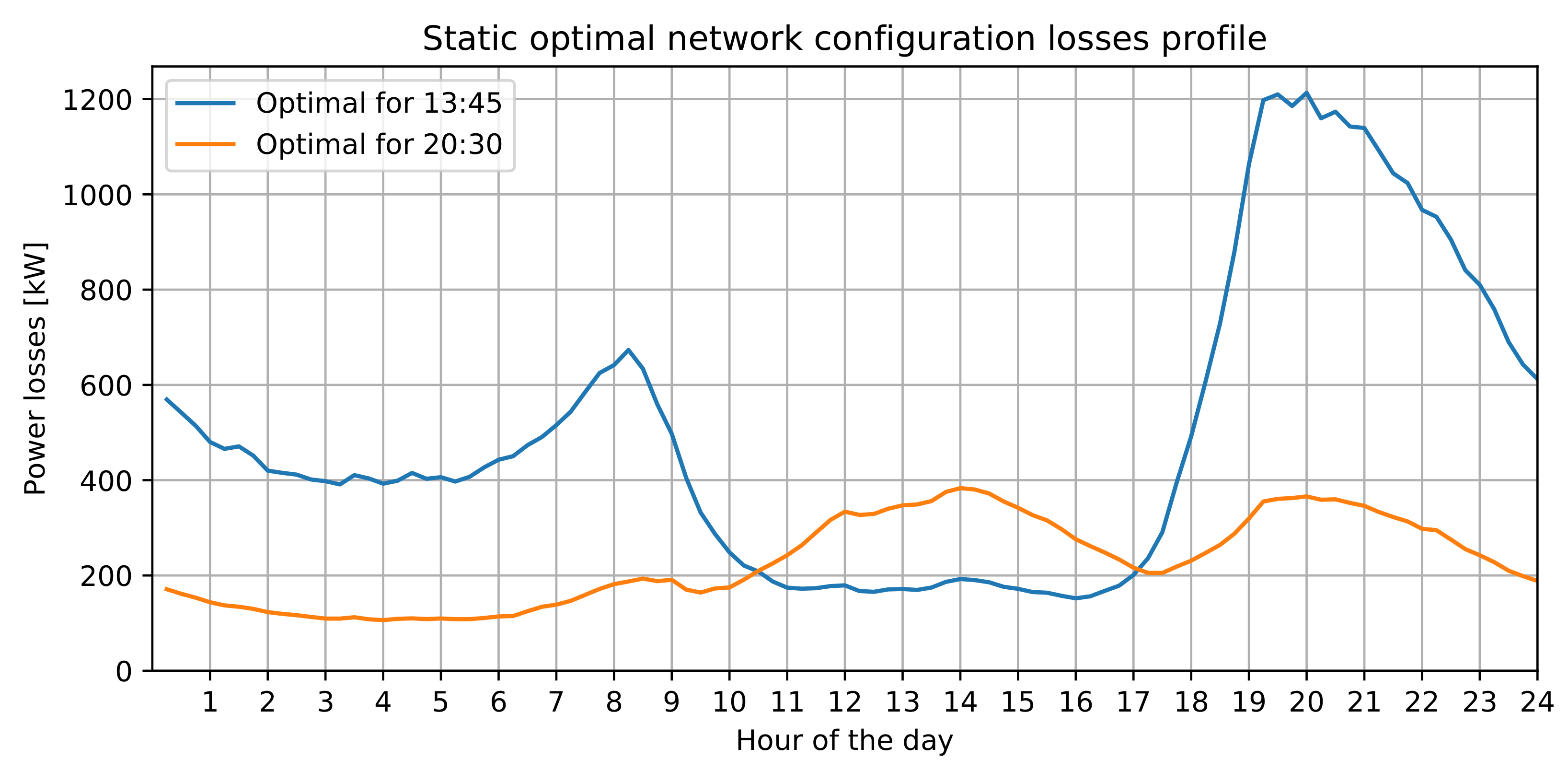
3.3. Static Optimal Network Configuration

The optimized network configuration for the net load profile at a particular time is given by (3). Given the asynchronism between net load profiles introduced by PV generation, the optimal configurations for the PV peak time and for the night load peak time are very distinct. Figure 2 shows the losses profile obtained for two different optimal configurations: one optimized at 13:45 and another optimized at 20:30. As expected, each configuration performs better than the other in the vicinity of the period for which it was optimized. This shows that none of these configurations alone would be optimal for the whole day as a static configuration, and that a dynamic configuration that would swap between the two configurations could bring significant benefits throughout the day.

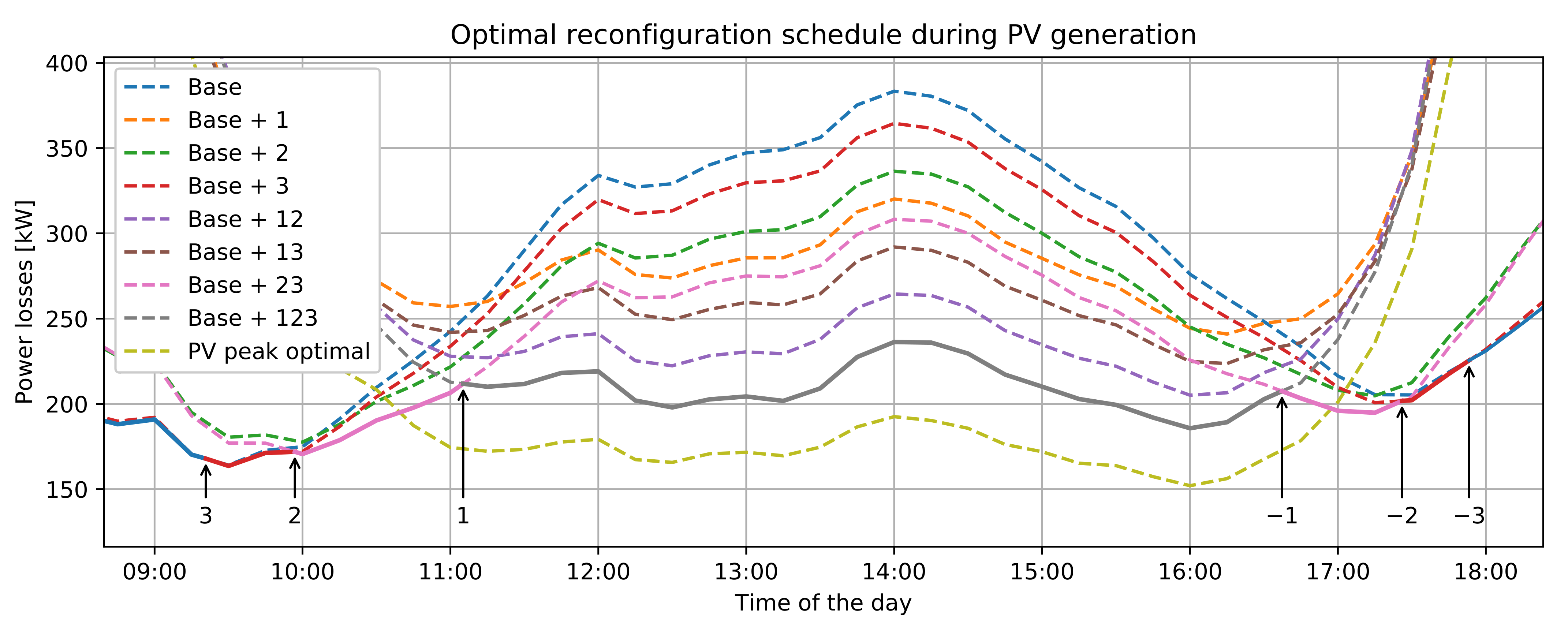
3.4. Dynamic Reconfiguration

As pointed out in Section 2, if there was no limitation on the number of switching operations, the network could be optimized in each time of the day and reconfigured successively from optimal to optimal in time. Since this limitation exists and the general optimization problem is too hard to be addressed as such, our approach is to use the optimal configurations for the PV peak time and for the night load peak time as the end-point configurations of a partial reconfiguration path to be carried out during the day. The length of this path is the number of switching operations we are allowed to make while transitioning from a daytime configuration to a night-time one, and the other way around to close the daily cycle. Since these two configurations are very different, a complete path between them may not be possible to undertake for being longer than the partial path we are allowed to do. Thus, this partial path cannot reach both end-point configurations, but it can reach one of them—the base configuration.

The best choice for the base configuration is the end-point configuration performing better for the whole day. Figure 2 clearly shows that the night-time optimal configuration is the best in terms of losses for the complete day. Additionally, the daytime optimal configuration performs much worse at night-time (with losses 800 kW higher than the other configuration) than the night-time optimal configuration does at PV peak time (with losses 200 kW higher than the other configuration). As such, we chose the night-time optimal configuration as the base configuration from which a reconfiguration path will be found towards the daytime optimal configuration, but not reaching it, given the limitation on the number of switching operations to perform.

The reconfiguration path from the base configuration (night-time) to a daytime configuration is an ordered sequence of switching operations to be performed over the base configuration. This path becomes a reconfiguration schedule when each switching operation is assigned to a particular point in time. For this illustrative example, we considered only the three most beneficial switching operations at the PV peak time from all the differences between the base configuration and the daytime optimal configuration. Thus, the reconfiguration schedule to be found has, at most, three switching operations, labeled 1, 2 and 3.

We then evaluated the losses profile for all eight possible subsets of these three operations (∅, {1}, {2}, {3}, {1,2}, {1,3}, {2,3}, {1,2,3}) when performed over the base configuration. Figure 3 shows these profiles on daytime period including both night-time to daytime and daytime to night-time transition periods. The optimal network configuration at a given time is the one with the lowest losses (excluding the PV peak optimal configuration which is plotted on Figure 3 just as a reference). As the optimal configuration is changing throughout the day, the reconfiguration schedule contains the switching operations, which perform the change. The path of this daily schedule is:

Base $\stackrel{3}{\to }$ Base + 3 $\stackrel{2}{\to }$ Base + 23 $\stackrel{1}{\to }$ Base + 123 $\stackrel{-1}{\to }$ Base + 23 $\stackrel{-2}{\to }$ Base + 3 $\stackrel{-3}{\to }$ Base

where the transition arrows indicate the switching operation done (positive values) or reverted (negative values) on that transition.

3.5. Energy Losses Dependence on Reconfiguration Schedule

It is clear from Figure 3 that, among the possible configurations obtained with three switching operations, the Base + 123 configuration remains the optimal configuration during most of the PV generation period. That schedule could be simplified. The reconfiguration could be modified to change the Base configuration onto the Base + 123 configuration with fewer time steps (but with the same total number of switching operations—three). As an example, with a single time step, all three switching operations could be undertaken at the same time—the time where the Base losses profile intercepts the Base + 123 profile in Figure 3. The search for simplified schedules would allow the problem to be formulated in an easier way but the resulting schedules would increase energy losses—note that the area under the corresponding profiles would be higher than the one obtained for the optimal schedule.

Figure 3. Losses profile for the considered network configurations. The optimal reconfiguration schedule encompasses several of these configurations—the profile resulting from the optimal schedule of such configurations is plotted as a solid line. The annotated points indicate the timing of each switching operation (1, 2 and 3). Negatively valued labels ($-1$, $-2$ and $-3$) indicate the timing chosen to revert the operations annotated beforehand. Data obtained from DPlan—Distribution Planning.

Figure 3. Losses profile for the considered network configurations. The optimal reconfiguration schedule encompasses several of these configurations—the profile resulting from the optimal schedule of such configurations is plotted as a solid line. The annotated points indicate the timing of each switching operation (1, 2 and 3). Negatively valued labels ($-1$, $-2$ and $-3$) indicate the timing chosen to revert the operations annotated beforehand. Data obtained from DPlan—Distribution Planning.

It is also clear from Figure 3 that, if we allow the inclusion of the PV peak optimal configuration in a schedule instead of the Base + 123 configuration (removing the limit of three switching operations), a reduction in energy losses would be expected. That would, however, make the optimization problem more complex, rather than simplifying it.

Thus, the problem simplifications, either those that reduce the time-resolution of switching, or those that reduce the number of switching decisions, contribute to deteriorate energy losses.

Table 2. Energy losses reduction for each schedule compared with the static Base optimal configuration.

Reconfiguration Schedule	Energy Losses Reduction [%]
Base $\stackrel{\mathrm{all}}{\to }$ PV peak optimal $\stackrel{-\mathrm{all}}{\to }$ Base	16.33
Optimal schedule with switching operations 1,2,3	12.54
Base $\stackrel{2,3}{\to }$ Base + 23 $\stackrel{1}{\to }$ Base + 123 $\stackrel{-1}{\to }$ Base + 23 $\stackrel{-2,-3}{\to }$ Base	12.52
Base $\stackrel{3}{\to }$ Base + 3 $\stackrel{1,2}{\to }$ Base + 123 $\stackrel{-1,-2}{\to }$ Base + 3 $\stackrel{-3}{\to }$ Base	12.18
Base $\stackrel{1,2,3}{\to }$ Base + 123 $\stackrel{-1,-2,-3}{\to }$ Base	12.02

shows the energy losses reduction found for the optimal schedule presented in the previous section and for the alternative schedules mentioned in the above discussion. The results are presented as a percentage of the energy losses obtained for the static Base configuration.

4. Problem Complexity and New Computation Paradigms

Table 3. Time complexity for the formulated problems, where p is the number of time steps, $\left|O\right|$ is the number of given switching operations (i.e., differences between two given network configurations) and m is the maximum number of switching operations to be found.

Problem	Time Complexity
	Number of Operations	Operation
Unrestricted optimal reconfiguration	p	optimization
Optimal static configuration	1	optimization
Time-bounded linear dynamic reconfiguration	$p^{\left|O\right|+1}$	power-flow
Time-unbounded cyclic dynamic reconfiguration	$p{\left(1+\frac{p(p-1)}{2}\right)}^{\left|O\right|}$	power-flow
Open cyclic dynamic reconfiguration	${\left(1+\frac{p(p-1)}{2}\right)}^m$	optimization

summarizes the time complexity for the problems formulated in Section 2. This complexity is stated as the number of network configuration optimizations or the number of power-flow runs depending, respectively, on the search space of each problem, including the network configurations space, or not. As expected, the problem with the least restricted optimal reconfiguration, the open cyclic dynamic reconfiguration, is also the most demanding in computational terms with $O\left(p^{2m}\right)$ network optimization runs. Thus, the complexity of this problem scales polynomially with the number of time steps p and exponentially with the maximum number of switching operations m.

As an example, a time resolution on 15 min (as in the real data of the example illustrated in Section 3) results in $p=96$ time steps for the 24 h period. Considering at most a single switching operation ($m=1$), this problem already needs 4561 optimization runs to be solved. Assuming a computation time for each network optimization of 10 s (a typical value for a medium-sized network optimized on DPlan—Distribution Planning, running on a 3 GHz desktop computer), the single-operation reconfiguration problem needs 13 h to be completed. This means that the computation of the problem needs to start 13 h ahead of the optimal time for the single switching operation using load and PV forecast data. Although this is possible to achieve in practice, adding 13 h to the forecast time span degrades the reliability of this forecast. Nevertheless, the single-operation reconfiguration problem brings only a marginal energy losses reduction as Figure 3 shows when comparing Base + 1 (the best single-operation configuration) and Base + 123 (the best three operations configuration).

With a maximum of two switching operations, the problem would explode to 20.8 million optimization runs, or more than 6 years of computation time, which is obviously infeasible. In order to try to reduce time complexity, the number of time steps p may be decreased.

Table 4. Time complexity for the open cyclic dynamic reconfiguration problem for some combinations of m and p.

Switching Operations	Time Steps	Time Complexity
m	p	Optimizations	Computation Time
1	96	4561	13 h
1	48	1129	3 h
1	24	277	46 min
1	12	67	11 min
2	96	20.8 M	6 years
2	48	1.3 M	5 months
2	24	76,729	9 days
2	12	4489	12 h
3	12	300,763	35 days
3	6	4096	11 h

shows the time complexity for some combinations of m and p. For three switching operations, the computation time would be feasible with, at most, 6 time steps. If evenly distributed over the 24 h, the time resolution with six time steps is 4 h. One could optimize the locations of the six time steps by concentrating three on them on the night-time to daytime transition period and the remaining three on the other transition period, but this would still result in a poor time resolution, which would severely degrade the optimality of the found schedule.

New Perspectives to Handle Problem Complexity

As illustrated previously, the exponential scaling of the problem complexity with the number of switching operations renders the problem impossible to handle with more than a single operation without degrading time resolution. Making the computation parallel with multiple cores would not remove the exponential scaling of the problem since the computation time speed-up would be, at most, linear with the number of cores, as stated by Amdahl’s law. Thus, a new computation paradigm is needed to find an optimal multiple-operation schedule.

We propose the use of quantum computing to address this kind of problem [19,20]. Quantum computing has the potential to provide an exponential speed-up when compared to classical computing [21]. This speed-up lies on the unique phenomena of quantum superposition and quantum entanglement which enables the computation parallelization with an exponential scaling with the quantum hardware size (i.e., the number of qubits—quantum bits) as opposed to the linear scaling with the number of cores of classical computing.

Quantum computing is still in its infancy as we are in what is known as the NISQ era (Noisy Intermediate-Scale Quantum) [22]. Being noisy, the nowadays quantum computers are not as reliable as their classical counterparts, and being intermediate-scaled means that there is a limit on the size of the problems that quantum computers are currently able to handle. Nevertheless, quantum computers are getting larger and more reliable, and thus more powerful. Due to this evolution, it is expected that quantum supremacy will be reached in the future, when quantum computers will be able to solve problems which are still unsolvable in classical computing [22].

Quantum computers can already deal with reduced versions of real reconfiguration problems. These demonstration-sized projects can prove whether the original problem is amenable to quantum computing and they may also provide an estimate for the scaling of the limit of the problem size as a function of quantum hardware size and characteristics.

Quantum computing is divided in two main paradigms: quantum circuit (or gate) model and quantum annealing. While the quantum circuit model is able to handle more general quantum computation algorithms, quantum annealing has much more potential for solving discrete optimization problems, such as the studied reconfiguration problem. Thus, we will employ quantum annealing to handle this problem in our future work. As part of that work, we will adapt the problem formulation we introduced in this paper into a form that the quantum annealer can accept.

Quantum annealing is probabilistic in nature. A quantum annealer returns samples from the problem search space following, approximately, a Boltzmann distribution. Thus, the lower energy samples (i.e., lower cost solutions for the problem) are more likely than the higher energy ones. Since we are dealing with probabilistic samples, there is no guarantee of obtaining the global optimal solution on a given number of trials, but good enough solutions can be obtained. The characterization of how good is the best returned solution as a function of the number of trials (i.e., as a function of time) is crucial to make a fair comparison with the existing classical methods. This characterization will also be part of our future work.

The state of the art in quantum annealing is the D-Wave Advantage machine with 5000 qubits [23]. This machine is able to solve problems with up to 5000 binary variables (with limitations in how the variables interact with each other). It also possible to use a D-Wave hybrid solver service to handle larger problems or problems with a denser graph of variables interaction. This solver uses classical computation to assist quantum annealing in order to overcome some current limitations of the latter.

5. Conclusions

In this paper, the problem of optimal dynamic reconfiguration of distribution grids was formulated. The solution of the reconfiguration problem was illustrated on a real network with real load data and a heavy PV generation scenario. The illustration showed the potential benefits of optimal reconfiguration for losses reduction. It has also shown how the complexity of the optimal reconfiguration problem scales with the number of candidate switching operations, rendering the problem infeasible in practical terms with just three operations. To overcome practical infeasibility, new approaches based on quantum annealing are discussed and proposed as realistic candidates to the effective solution of the problem in the future. Our future work includes the reformulation of the problem for quantum annealing and the characterization of the quantum annealer performance when compared to existing classical methods.

References

1. Ilic, M.; Joo, J.; Carvalho, P.M.S.; Ferreira, L.A.F.M.; Almeida, B. Dynamic monitoring and decision systems (DYMONDS) framework for reliable and efficient congestion management in smart distribution grids. In Proceedings of the 2013 IREP Symposium Bulk Power System Dynamics and Control—IX Optimization, Security and Control of the Emerging Power Grid, Rethymno, Greece, 25–30 August 2013; pp. 1–9. [Google Scholar] [CrossRef]
2. Lueken, C.; Carvalho, P.M.; Apt, J. Distribution grid reconfiguration reduces power losses and helps integrate renewables. Energy Policy 2012, 48, 260–273, Special Section: Frontiers of Sustainability. [Google Scholar] [CrossRef]
3. Nižetić, S.; Papadopoulos, A.; Tina, G.; Rosa-Clot, M. Hybrid energy scenarios for residential applications based on the heat pump split air-conditioning units for operation in the Mediterranean climate conditions. Energy Build. 2017, 140, 110–120. [Google Scholar] [CrossRef]
4. Carvalho, P.M.S.; Ferreira, L.A.F.M. Large-Scale Network Optimization with Evolutionary Hybrid Algorithms: Ten Years’ Experience with the Electric Power Distribution Industry. In Computational Intelligence in Expensive Optimization Problems; Springer: Berlin/Heidelberg, Germany, 2010; pp. 325–343. [Google Scholar] [CrossRef]
5. Meng, X.; Zhang, L.; Cong, P.; Tang, W.; Zhang, X.; Yang, D. Dynamic reconfiguration of distribution network considering scheduling of DG active power outputs. In Proceedings of the 2014 International Conference on Power System Technology, Chengdu, China, 20–22 October 2014; pp. 1433–1439. [Google Scholar] [CrossRef]
6. Capitanescu, F.; Ochoa, L.F.; Margossian, H.; Hatziargyriou, N.D. Assessing the Potential of Network Reconfiguration to Improve Distributed Generation Hosting Capacity in Active Distribution Systems. IEEE Trans. Power Syst. 2015, 30, 346–356. [Google Scholar] [CrossRef]
7. Jakus, D.; Čađenović, R.; Vasilj, J.; Sarajčev, P. Optimal Reconfiguration of Distribution Networks Using Hybrid Heuristic-Genetic Algorithm. Energies 2020, 13, 1544. [Google Scholar] [CrossRef] [Green Version]
8. Čađenović, R.; Jakus, D.; Sarajčev, P.; Vasilj, J. Optimal Distribution Network Reconfiguration through Integration of Cycle-Break and Genetic Algorithms. Energies 2018, 11, 1278. [Google Scholar] [CrossRef] [Green Version]
9. Huang, W.T.; Chen, T.H.; Chen, H.T.; Yang, J.S.; Lian, K.L.; Chang, Y.R.; Lee, Y.D.; Ho, Y.H. A Two-stage Optimal Network Reconfiguration Approach for Minimizing Energy Loss of Distribution Networks Using Particle Swarm Optimization Algorithm. Energies 2015, 8, 13894–13910. [Google Scholar] [CrossRef] [Green Version]
10. Kaur, M.; Ghosh, S. Effective Loss Minimization and Allocation of Unbalanced Distribution Network. Energies 2017, 10, 1931. [Google Scholar] [CrossRef] [Green Version]
11. Mishra, S.; Das, D.; Paul, S. A comprehensive review on power distribution network reconfiguration. Energy Syst. 2017, 8, 227–284. [Google Scholar] [CrossRef]
12. Carvalho, P.; Ferreira, L.; Barruncho, L. Optimization approach to dynamic restoration of distribution systems. Int. J. Electr. Power Energy Syst. 2007, 29, 222–229. [Google Scholar] [CrossRef]
13. Xu, L.; Cheng, R.; He, Z.; Xiao, J.; Luo, H. Dynamic Reconfiguration of Distribution Network Containing Distributed Generation. In Proceedings of the 2016 9th International Symposium on Computational Intelligence and Design (ISCID), Hangzhou, China, 10–11 December 2016; Volume 1, pp. 3–7. [Google Scholar] [CrossRef]
14. Guimarães, I.G.; Bernardon, D.P.; Garcia, V.J.; Schmitz, M.; Pfitscher, L.L. A decomposition heuristic algorithm for dynamic reconfiguration after contingency situations in distribution systems considering island operations. Electr. Power Syst. Res. 2020, 2020, 106969. [Google Scholar] [CrossRef]
15. Košt’álová, A.; Carvalho, P.M. Towards self-healing in distribution networks operation: Bipartite graph modelling for automated switching. Electr. Power Syst. Res. 2011, 81, 51–56. [Google Scholar] [CrossRef]
16. Łukaszewski, A.; Nogal, Ł.; Robak, S. Weight Calculation Alternative Methods in Prime’s Algorithm Dedicated for Power System Restoration Strategies. Energies 2020, 13, 6063. [Google Scholar] [CrossRef]
17. QGIS Project. Available online: https://qgis.org (accessed on 30 December 2020).
18. OpenStreetMap. Available online: https://www.openstreetmap.org (accessed on 30 December 2020).
19. Nielsen, M.A.; Chuang, I.L. Quantum Computation and Quantum Information: 10th Anniversary Edition; Cambridge University Press: Cambridge, UK, 2010. [Google Scholar] [CrossRef] [Green Version]
20. Biswas, R.; Jiang, Z.; Kechezhi, K.; Knysh, S.; Mandrà, S.; O’Gorman, B.; Perdomo-Ortiz, A.; Petukhov, A.; Realpe-Gómez, J.; Rieffel, E.; et al. A NASA perspective on quantum computing: Opportunities and challenges. Parallel Comput. 2017, 64, 81–98, High-End Computing for Next-Generation Scientific Discovery. [Google Scholar] [CrossRef] [Green Version]
21. Zhou, L.; Wang, S.T.; Choi, S.; Pichler, H.; Lukin, M.D. Quantum Approximate Optimization Algorithm: Performance, Mechanism, and Implementation on Near-Term Devices. Phys. Rev. X 2020, 10, 021067. [Google Scholar] [CrossRef]
22. Preskill, J. Quantum Computing in the NISQ era and beyond. Quantum 2018, 2, 79. [Google Scholar] [CrossRef]
23. D-Wave Advantage™ Quantum Annealer. Available online: https://www.dwavesys.com/d-wave-two%E2%84%A2-system (accessed on 26 January 2021).
Figure 1. The studied 15 kV distribution grid. The network arcs are colored by feeder circuit. (a) Complete network; the city center is highlighted with the black rectangle. Note the scale on the lower right corner. (b) Detail of the highlighted city center with the selected buildings for PV generation (green outline) and PV injection points on the grid (red dots). Images obtained from DPlan—Distribution Planning and QGIS.
Energies 14 00830 g001
Figure 2. Losses profile for static network configurations. Data obtained from DPlan—Distribution Planning.
Energies 14 00830 g002