Abstract
This paper introduces a sliding-mode-based extremum-seeking algorithm aimed at generating optimal set-points of wind turbines in wind farms. A distributed extremum-seeking control is directed to fully utilize the captured wind energy by taking into consideration the wake and aerodynamic properties between wind turbines. The proposed approach is a model-free algorithm. Namely, it is independent of the model selection of the wake interaction between the wind turbines. The proposed distributed scheme consists of two parts. A dynamic consensus algorithm and an extremum-seeking controller based on sliding-mode theory. The distributed consensus algorithm is exploited to estimate the value of the total power produced by a wind farm. Subsequently, sliding-mode extremum-seeking controllers are intended to cooperatively produce optimal set-points for wind turbines within the farm. Scheme performance is tested via extensive simulations under both steady and varying wind speed and directions. The presented distributed scheme is compared with a centralized approach, in which the problem can be seen as a multivariable optimization. The results show that the employed scheme is able to successfully maximize power production in wind farms.
1. Introduction
Grouping wind turbines into wind plants (or farms) is one of the most effective ways to produce energy from wind. It helps to reduce the operational and maintenance cost, usage of land and consequently produce affordable green and renewable energy. However, in a wind farm, the kinetic energy is extracted from the wind flow by wind turbines; therefore, the turbine on the upwind side reduces the wind speed before reaching the wind turbines in the downwind side of the farm. Thus, conventional control and optimization methods that optimized a stand-alone wind turbine system and neglect the aerodynamic wake interaction among wind turbines when maximizing the energy captured by wind farms provide a sub-optimal solution. On the other hand, modeling such an interaction remains a difficult task. This introduces the necessity to employ a model-free optimization method to search for optimal set-points of wind turbines in the wind farm.
Extremum-seeking (ES), also known as self-optimization, control can be categorized as a class of optimal control that concerns the situation when the performance function to be optimized is available for measurement but not exactly known. From another perspective, ES control is an adaptive control method in which the control aim is to drive the system output to track undetermined optimal operating points or settings. The first sliding-mode gradient-free optimization method was proposed by Korovin and Utkin in [1]. The key concept is to design a variable structure control (VSC) so that the system output, i.e., the cost function to be optimized, tracks a monotonic function in time in the direction of the optimal point. Later, the method was generalized as ES control with sliding modes for general nonlinear systems by Özgüner and his coworkers. At first, a periodic search (sinusoidal) function was introduced in [2] and analyzed further in [3]. Then, stability analysis considering different scenarios was studied in [4]. Gradient estimation and a discrete sliding mode ES method were proposed in [5]. In terms of applicability of the method, the sliding-mode-based ES has a wide scope of applications in many areas, for example, automotive [6], robotics [7], and renewable energy systems for both, solar [8] and wind [9]. Recently, different multivariable sliding-mode-based ES control schemes were proposed and analyzed. The first scheme was proposed in [10] where the author proposed a multivariable sliding mode ES with application in Raman optical amplifiers. Another scheme was proposed in [11] for an alternator maximum power point tracking (MPPT). A sequential approach was proposed and analyzed in [12] with application in wind farm power maximization. A common limitation of these schemes is the fact that these multivariable schemes are centralized in nature and the weak coupling assumption. Other than the sliding-mode-based ES control, the literature currently features many design approaches for ES control. A well-known approach is the sinusoidal perturbation method, which was proposed in [13], a nonlinear programming based method [14], Newton-based ES [15], and a Shahshahani gradient ES [16], to name a few.
The literature on the model-free distributed optimization methods for maximizing power extracted from the wind farms shows a multitude of methods. The key idea is to design an algorithm that coordinates and generates the control set-point for an individual wind turbine by considering the wake and aerodynamic properties between the farm’s turbines. Particularly, the goal is to reduce the extracted power from the upwind turbines, allowing the downwind tribunes to extract more energy. To achieve this, the axial induction factor (AIF) is considered the control input for an individual wind turbine. Using recent results in game theory, two learning algorithms were employed for wind farm optimization in [17]. The difference between the two algorithms is with regard to the communication structure and the available information to each decision maker, i.e., controller or agent. In the same context, a cooperative game approach was proposed in [18]. The author used both the yaw offset angles as well as the axial induction factor to optimize the power production. A new data-driven approach was proposed in [19]. The author developed two gradient-based maximum power point tracking (MPPT) schemes that were based on the measurement of the wind speed at the upwind side and the estimation of the average wind speed in the farm [20]. As far as the ES algorithms are concerned, sinusoidal-perturbation-based ES control schemes were proposed in [21,22,23,24] where the authors proposed to introduce a consensus mechanism to exchange information, in real-time, about the value of total performance function among the wind turbines.
In this work, a distributed ES control based on sliding-mode theory is employed to generate the wind turbine axial induction factor and influence the overall performance of the wind farm. The key concept behind this approach is the introduction of a consensus dynamic in order to estimate the average value of the total generated power. Then, the dynamic is suitably interfaced with sliding-mode-based extremum-seeking controllers to obtain the optimal settings. One of the main contributions of this paper is the development of a model-free optimization method via distributed sliding-mode-based ES for wind farm optimization. This paper extends, from the application point of view, the results presented in [25]. Compared with the existing works, the proposed solution is distinguishable in several aspects: First, it is an extension to the centralized multivariable ES control schemes proposed in [12] for wind farm optimization problems. Although the centralized ES approach has proven to be effective in many areas, distributed optimization approaches and decentralized schemes improve the scalability of systems. Second, we compared with the results proposed in [26] to find Nash solution in a non-cooperative game and considering that the Nash solution is not the socially optimal solution, this paper seeks to extend the result using the newly developed cooperative ES control [25] to solve the optimization problem in a cooperative fashion. Third, in contrast to existing works in distributed ES [27,28,29] and wind farm optimization [21,22,24,30] that build on the sinusoidal-perturbation approach, this work employs a sliding-mode-based ES control. The sliding-mode approach has the potential to simplify the implementation and improve the convergence rate. Forth, compared with the work proposed by [9] to optimize a stand-alone wind turbine using a single variable-sliding-mode ES, this work investigates the problem optimizing a wind farm using a multivariable ES. Finally, the implementation section features different simulation scenarios. The proposed scheme was tested under both fixed and varying wind speeds. Then, the proposed distributed scheme is compared with both the Nash-based ES control scheme and the centralized ES approach.
2. Wind Farm Model and Optimization
In this section, we explicate the nature of the problem concerning optimizing a wind farm. In wind farms, the kinetic energy of moving air is extracted by the wind turbines and, consequently, wind is slower after passing through the blades. In other words, the wind speed is reduced in the wake downstream of the wind turbine routers by the wind turbine. This phenomenon is called the wake effect. It reduces the power production of the overall farm due to the decrease in wind speed. By taking into consideration the wake and aerodynamic properties among wind turbines in a farm, a recent result [31] shows that an energy gain of more than ten percent can be achieved, in comparison to the existing National Renewable Energy Laboratory (NREL) controller. This section overviews the wind turbine modeling and control. Then, it previews the wind farm optimization problem.
In this work, a farm consists of an array of n connected wind turbines with the full wake effect considered. As can be seen in Figure 1, the considered configuration is not restrictive, since many wind farms can be grouped to form series-connected turbines.
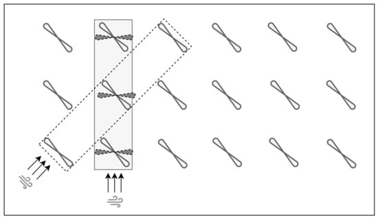
Figure 1.
Grouping wind turbines into a set of series-connected turbines with full wake effect for different orientation, depending on the wind direction.
2.1. Wind Turbine Control
Concerning the power control in wind turbines, three types of control can be found in the literature. Yaw-, pitch-, and torque-based control methods. Yaw-based control, i.e., changing the rotor direction, is a slow method when compared to other control actions and, therefore, it does not influence power production in a wind farm as fast as other actions. On the other hand, pitch and torque control can be related if the problem is formulated in terms of the axial induction factor.
The wind turbine’s axial induction factor is a non-dimensional ratio that expresses the decrease in the wind velocity between the free stream and the rotor plane. It is used as a high-level control input (set-point) to influence the generated power in wind farms (see, for example, ref. [32]). It is a function of two quantities that can be controlled by low-level controllers: The turbine’s blade pitch angle and tip-speed ratio . The tip-speed ratio is a function of the undisturbed wind speed V, rotor’s angular velocity , and rotor radius R:
The control strategy of a wind turbine depends on the wind speed. The tip-speed ratio can be adjusted by means of torque control when the wind speed is below the rated value, known as Region-2. On the other hand, blade pitch angle is one of the control inputs when the wind speed is above the rated speed. Details about the wind turbine’s region of operation can be found in [33]. This gives a general idea on how the axial induction factor is manipulated.
Remark 1.
The focus in this work is on the design of a high-level controller that generates set-points that can be tracked by low-level controllers, depending on the turbine specifications.
2.2. Wake Interaction Model
The most challenging part of optimizing a wind farm is modeling the wind velocity profile with the consideration of wake created by multiple wind turbines. A well-studied wake model in the area of wind energy, known as Park model [17,34], is considered in the paper. For each wind turbine i, the effective wind velocity is given by the following:
where is the free stream wind speed, is the axial induction factor (to be described later), and represents the velocity defects seen by turbine i, which is given by
where is a matrix that depends on the layout of the wind farm, (i.e., distance between turbines and the interacting wakes) and given by
where is the diameter of the surface area (disk) produced by the blades of turbine j. is the surface area of disk produced by the blades of the wind turbine i and is the region of overlap between the wake produced by the wind turbine j and the surface area produced by the blades of turbine i.
Remark 2.
The proposed ES control scheme is a model-free method, meaning that it is independent of the model selection of the wake interaction. The selected model is used for simulation and results verification.
2.3. Model of Produced Power
For each turbine i, let the axial induction factor, denoted by , be the control parameter, which takes values in . is given by
where is the wind speed at the rotor. The power produced by each turbine can be written in terms of the axial induction factor as
where:
- is the air’s density.
- is the area swept by blades of turbine i.
- is the power efficiency coefficient, which given by
2.4. Optimization Problem
The problem concerning optimization of the power generated by a wind turbine can be categorized into two main paths. First, optimizing a stand-alone wind turbine system in which the goal is to maintain the power efficiency coefficient as close to Betz’s coefficient at , also known as Maximum Power Point Tracking (MPPT) problem (see, for example, ref. [9]). The other path, which is the subject of this work, is concerning the coordination (cooperation) between individual turbines in order to optimize the total power generated by the Farm and generate a new optimal set values of axial induction factors. Figure 2 presents this fact for the case of two turbines. It is evident that the total power generated by the two turbines is maximized in the event that the upwind turbine operates below its maximum operation point, i.e., is less than .
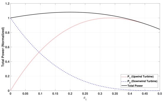
Figure 2.
The effect of the wake and aerodynamic properties between two turbines. Setting will maximize the power of the first turbine (solid red); however, it will reduce the total generated power (solid black).
In this paper, an array of n wind turbines standing in the wake of each other is considered. Each turbine is associated with a controller, and will be refereed to as agents. Each agent i for is able to measure its local cost function for the turbine i. In addition, agents have the capability to exchange information over a fixed, time-invariant, undirected, and strongly connected graph . is the vertex set representing the number of agents. is the edge set. Considering that it is crucial to accurately model the interaction among the wind turbines in a farm, agent i is assumed to be able to measure the power produced by turbine i rather than estimate the power. The optimizing problem is to maximize the power produced by the farm which is given by
3. Proposed Optimization Strategy
To maximize the energy captured in a wind farm, each agent is required to act in a cooperative manner. In order to achieve cooperation between agents, a consensus protocol is introduced such that all agents can have a good estimate of the total power produced by the farm (8). After that, the goal of each agent is to optimize, in real-time, a multivariable cost function. In the designed coordination scheme, the consensus protocol ensures that each agent receives an estimate of the average of the total cost function via a distributed algorithm. Then, a sliding-mode-based extremum-seeking controller utilizes the received estimate to update the consensus with a new value as a new decision has been taken by the local sliding-mode extremum-seeking controller.
Assumption 1.
Each agent is able to communicate with its neighbors and estimate the average of the total cost function .
This assumption is reasonable due to the fact that modern wind turbines are equipped with communication equipment to transmit and receive all operational signals. In case of communication loss, the proposed scheme will produce a non-cooperative solution. Under Assumption 1, agent i measures the average of the total cost function, , by running a distributed dynamic consensus algorithm. In particular, the dynamic average consensus protocol proposed by Freeman et al. [35] is utilized in this work. A dynamic average consensus algorithm is used to make sure that the consensus algorithm is, continually, driven by the inputs in real-time such that the average of the changing inputs is tracked. The consensus protocol is given by the following:
where is the estimated cost function for agent i, is an auxiliary state, is the dynamic input, and is a global parameter. The dynamic can be rewritten in compact form as follows:
where , and is the integral Laplacian, constructed form the weights , and is the proportional Laplacian, constructed form the weights . For this approach, is chosen to be the input to the dynamic .
A basic sliding-mode-based extremum-seeking scheme for general nonlinear system is shown in Figure 3. The key concept behind the sliding mode ES is to design a variable structure control input such that the measured performance (cost) function tracks a monotonic function in time towards the optimal points. In the case of maximization problem, the controller follows an increasing function. To design an extremum-seeking controller with sliding mode, a switching function for the agent is defined as follows:
where is a reference signal that satisfies:
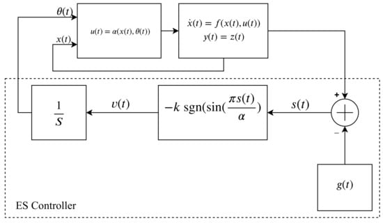
Figure 3.
Block diagram for sliding-mode-based extremum-seeking control for a general nonlinear system.
That is, is a monotonic increasing function of time. Next, let the axial induction factor, be defined as
where is a variable structure law selected as
where and are positive design parameters. The controller design section is concluded with the following assumption about the controller.
Assumption 2.
The consensus dynamic (11) is much faster than the one of the ’s dynamics, that is,
This assumption ensures a time-scale separation between the consensus dynamic and the ES controller. This assumption is reasonable and can be done by choosing a small k for each ES controller. In other words, the ES controller gain k shall be chosen to be much smaller than the consensus parameters.
4. Controller Analysis
The aim of this section is to show that the output of the proposed scheme converges to a vicinity of points that maximizes the value of . This will be shown in two main steps. First, the convergence of the consensus algorithm is highlighted. Second, the sliding-mode existence condition need to be studied.
Lemma 1.
Consider the consensus system (11) and let the graph G be a fixed, undirected and strongly connected graph. Then, for any initial conditions, the system states remain bounded and each state converges exponentially to as .
Proof of Lemma 1.
The proof can be found in [35]. It is worthwhile to mention that this result holds for slowly varying input only. □
Using this lemma and under Assumption 2, we have
Therefore, throughout this section of analyzing the slow dynamics, is considered as the measured cost function for each agent i. The condition for the sliding mode to take place is that the deviation from the switching surface and its derivative should have the opposite sign in the vicinity of the switching surface . In other words, if there exists a constant number such that:
then, the sliding mode will exist at (see, for details, [4]). To this end, the following lemma summarizes the sliding-mode existence conditions.
Lemma 2.
For each agent i, with the switching function (12) and ES control input (15). Let the local cost functions be concave functions and the solution to the problem (8) exist, being unique and finite. Then, the sliding mode-existence condition is ensured and kept on manifold given by if the following conditions hold:
- For the given cost function (6), the sum of the absolute values of the partial derivative with respect to is greater than , i.e.,
- The ES controller parameter is chosen such that:
Proof of Lemma 2.
The proof can be found in [25]. □
Different from the classical sliding mode, the ES controllers are sliding on a number of sliding surfaces while searching for the optimal settings. As long as the sliding mode is active, the switching surface will be constant; accordingly, the cost function will follow the monotonic increasing function towards a vicinity of the optimal solution. After entering the vicinity, which is defined by the region (19), it is possible that either the system output stays inside that vicinity or goes through it. In the latter case, another sliding mode will take place and the system will re-enter the vicinity again on the sliding mode.
5. Implementation and Simulation
The implementation of the proposed scheme is presented for different scenarios of the problem of maximizing power extraction from the wind in a farm. First, the case with fixed wind speed is considered. Then, the case where the wind speed changes over time is implemented. Finally, the decentralized approach is compared with the centralized approach presented in [12]. It is assumed that all turbines are alike and each turbine is equipped with necessary tools for communication and sensing.
More specifically, three wind turbines are considered for simulation, shown in Figure 4. The turbines are assumed to have identical diameter m. Wind turbines are spaced apart by a distance equal to five-times the diameters. That is, the turbines are placed at . The air density is fixed to be equal to 1.225 kg/m3. In addition, each turbine can exchange information with its close neighboring turbines. For this setup, a Laplacian matrix L is given by the following:
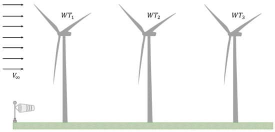
Figure 4.
Visualization of layout of the simulated wind farm. The farm comprises of three turbines connected in series.
Scheme gains and parameters are set as , , , and . In order to satisfy Assumption 2, the ES controller gain k is chosen to be much smaller than the consensus parameters. This will ensure that a consensus is reached in a short time. The implementation scheme is shown in Figure 5. As noted before, the optimal setting of an individual turbine can be determined from (6) and (7). Namely, Since this is an optimal solution for a stand-alone turbine, setting all is considered a non-cooperative solution (greedy control strategy). However, if the optimal settings for the total produced power by the farm’s turbines are taken into account, then optimizing the following multivariable function shall be considered:
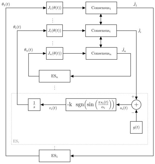
Figure 5.
Implementation of the proposed distributed ES Control.
Using a numerical optimizer to maximize the above equation yields an optimal setting given by , and . Optimizing the wind farm under a fixed free stream wind speed of is considered first. Sliding-mode existence is observed in Figure 6. Different from the convergence behavior of a classical first-order sliding mode controller, the ES controllers slide on several sliding surfaces while searching for the optimal settings, i.e., the optimization process, until reaching the proximity of the optimal settings. Once the maximum output is reached, the function gradient will be small enough such that the sliding-mode existence condition (19) will be no longer valid, and hence will be decreasing. The idea of sliding on several surfaces can also be observed in the convergence behavior of shown in Figure 7a. The initial values were chosen such that individual turbines are optimal, i.e., . converges to , as demonstrated in Figure 7b, since the farm is not affected by the last turbine. In selecting the controller parameters, different frequencies are utilized, by selecting different , in accordance to Lemma 2. Figure 8 shows the power generated by each wind turbine (WT) along with the corresponding axial induction factor. One can observe that the ES controller set the upwind turbine (WT1) to operate at lower capacity, allowing for high wind speed to pass to the downwind turbines. Two control strategies are compared in Figure 9. Namely, the proposed decentralized control is compared with the centralized scheme proposed in [12]. Starting from an optimal setting for individual turbines, the proposed controllers are able to improve the total captured energy by the farm. The power output significantly increased and reached the proximity of the maximum value. Since this is a derivative-free algorithm, the ES controllers can only identify a vicinity of the optimal solution and, therefore, the outputs have noticeable oscillation around the maximum value.
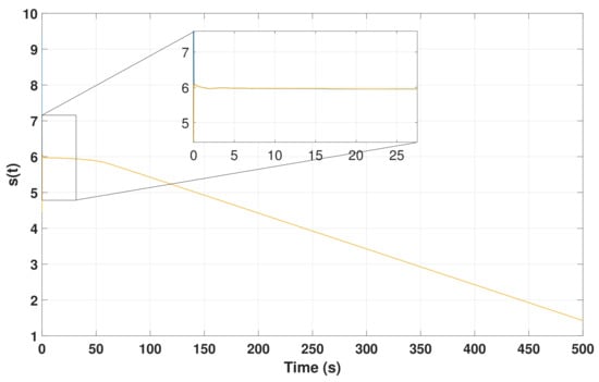
Figure 6.
Switching functions for each agent with the distributed sliding-mode extremum-seeking control. The sliding-mode existed during the search phase (zoomed figure).
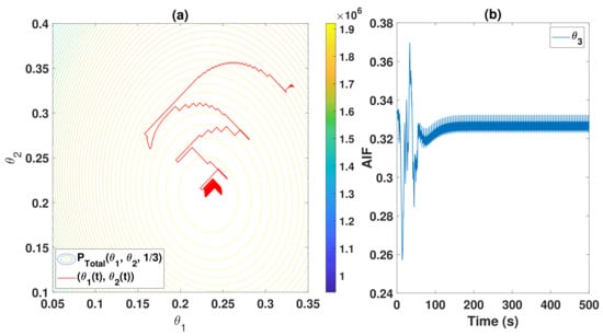
Figure 7.
Convergence of the axial induction factors using the proposed distributed scheme. (a) For the first two turbines with, . (b) Convergence of .
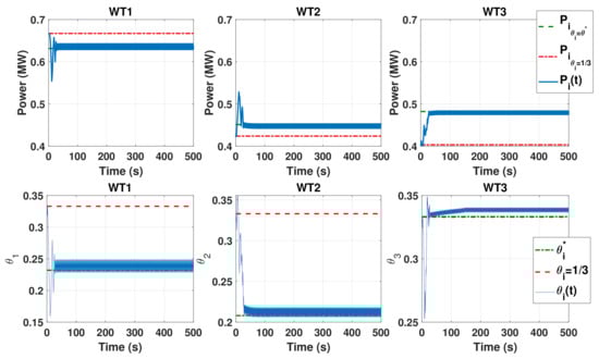
Figure 8.
Power output of the three wind turbines along with the corresponding axial induction factor generated by the proposed scheme.
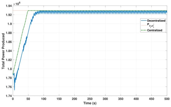
Figure 9.
Maximizing the total produced power the proposed method (solid) versus the centralized approach (dotted).
Remark 3.
The observed oscillation is natural, yet it can be lowered by reducing both parameters, and k. However, it will result in a slow convergence, see [4] for details.
It should be noted that there is also a trade-off between the scheme’s speed of convergence and the speed of the consensus dynamics. Moreover, it can be observed that the centralized approach provides a more accurate control input as well as a faster convergence, especially for small-scale problems. However, besides the reliability issues associated with the centralized schemes, recall that the decentralized method shows two major advantages in comparison with the centralized architecture. It is computationally less expensive, and in practice, easier to implement. Maximizing the total generated power using the proposed control scheme is compared with the total power generated by applying a non-cooperative control [26] in Figure 10 for a different wind direction. Assuming a fixed yaw angle, the wind direction affects the overlap area between the wake produced by the upwind wind turbine and the (surface area) disk produced by the blades of the downwind wind turbine. A 100 percent overlapping corresponds to the setup in Figure 4, where a zero percent overlapping means that the air direction is perpendicular to the turbines. What is interesting in this comparison is that control strategies only coincide under zero overlapping. Finally, the performance of the designed controller under a time-varying cost function is investigated. In this setup, the wind speed is varied periodically over time to test the robustness of the scheme. Figure 11 shows that the controller is able to track the optimal performance and maintain a maximum power production in the farm.
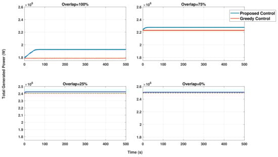
Figure 10.
Comparison between the proposed control scheme and the non-cooperative (Greedy control) scheme proposed in [26] for total power maximization under different wind directions.
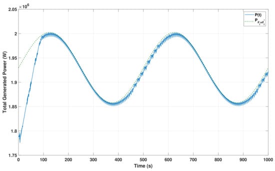
Figure 11.
Successful tracking of optimal production under varying free stream wind speeds.
6. Conclusions
The proposed optimization scheme attempted to develop a model-free approach towards maximizing power captured by a wind turbine farm, namely, through the adoption of a distributed sliding-mode extremum-seeking control scheme. In contrast to conventional control methods that typically optimize individual turbine performance, the proposed scheme maximizes overall captured power in a cooperative fashion, thereby accounting for turbine-to-turbine interactions and ambient conditions in order to reach an optimal set-point for each of the turbines available within the farm. The strategy of introducing a consensus algorithm as a dynamic mechanism to exchange information about the power produced by the farm has been considered. The problem is then reduced to a multivariable extremum-seeking control problem, which is solved by a sliding-mode extremum-seeking controller for each turbine. The stability and convergence of the proposed scheme have been discussed. Performance verification is conducted through a series of experiments and is compared versus several control architecture including centralized as well as non-cooperative schemes under a variety of wind conditions. While this real-time optimization using sliding-mode control highlights the potential of increasing captured power under steady-state conditions, future investigations should aim to further its extension into more adverse conditions in which performance might be disrupted by the presence of measurement noise, time-delay, and poor communication networks.
Author Contributions
Conceptualization, Y.B.S.; methodology, Y.B.S. and U.O.; software, Y.B.S.; validation, Y.B.S.; formal analysis, Y.B.S.; investigation, Y.B.S.; resources, Y.B.S. and U.O.; data curation, Y.B.S.; writing—original draft preparation, Y.B.S.; writing—review and editing, Y.B.S.; visualization, Y.B.S.; supervision, U.O.; project administration, Y.B.S. and U.O.; funding acquisition, Y.B.S. All authors have read and agreed to the published version of the manuscript.
Funding
This paper is supported by Reserechers Supporting Project number (RSP-2020/270), King Saud University, Riyadh, Saudi Arabia.
Institutional Review Board Statement
Not applicable.
Informed Consent Statement
Not applicable.
Data Availability Statement
Not applicable.
Conflicts of Interest
The authors declare no conflict of interest.
References
- Korovin, S.; Utkin, V. Using sliding modes in static optimization and nonlinear programming. Automatica 1974, 10, 525–532. [Google Scholar] [CrossRef]
- Drakunov, S.; Özgüner, Ü. Optimization of nonlinear system output via sliding mode approach. In Proceedings of the IEEE International Workshop on Variable Structure and Lyapunov Control of Uncertain Dynamical Systems, Sheffield, UK, 7–9 September 1992; pp. 61–62. [Google Scholar]
- Yu, H.; Ozguner, U. Extremum-seeking control via sliding mode with periodic search signals. In Proceedings of the 41st IEEE Conference on Decision and Control, Las Vegas, NV, USA, 10–13 December 2002; Volume 1, pp. 323–328. [Google Scholar]
- Pan, Y.; Özgüner, Ü.; Acarman, T. Stability and performance improvement of extremum seeking control with sliding mode. Int. J. Control 2003, 76, 968–985. [Google Scholar] [CrossRef]
- Fu, L.; Özgüner, Ü. Extremum seeking with sliding mode gradient estimation and asymptotic regulation for a class of nonlinear systems. Automatica 2011, 47, 2595–2603. [Google Scholar] [CrossRef]
- Yu, H.; Ozguner, U. Extremum-seeking control strategy for ABS system with time delay. In Proceedings of the American Control Conference, Anchorage, AK, USA, USA, 8–10 May 2002; Volume 5, pp. 3753–3758. [Google Scholar]
- Fu, L.; Ozguner, U. Extremum-seeking control in constrained source tracing with nonholonomic vehicles. IEEE Trans. Ind. Electron. 2009, 56, 3602–3608. [Google Scholar] [CrossRef]
- Alqahtani, A.H.; Utkin, V.I. Self-optimization of photovoltaic system power generation based on sliding mode control. In Proceedings of the IECON 2012-38th Annual Conference on IEEE Industrial Electronics Society, Montreal, QC, Canada, 25–28 October 2012; pp. 3468–3474. [Google Scholar]
- Shen, D.; Khayyer, P.; Izadian, A. Sliding mode extremum seeking control for maximum power point tracking in wind system. In Proceedings of the 2016 IEEE Power and Energy Conference at Illinois (PECI), Urbana, IL, USA, 19–20 February 2016; pp. 1–6. [Google Scholar]
- Peixoto, A.J.; Oliveira, T.R. Extremum seeking control via sliding mode and periodic switching function applied to Raman optical amplifiers. In Proceedings of the 2012 American Control Conference (ACC), Montreal, QC, Canada, 27–29 June 2012; pp. 5377–5382. [Google Scholar] [CrossRef]
- Toloue, S.F.; Moallem, M. Multivariable Sliding-mode Extremum Seeking Control with Application to MPPT of an Alternator-based Energy Conversion System. IEEE Trans. Ind. Electron. 2017, 64, 6383–6391. [Google Scholar] [CrossRef]
- Bin Salamah, Y.; Ozguner, U. Sliding Mode Multivariable Extremum Seeking Control with Application to Wind Farm Power Optimization. In Proceedings of the American Control Conference (ACC), Milwaukee, WI, USA, 27–29 June 2018; pp. 5321–5326. [Google Scholar]
- Ariyur, K.B.; Krstic, M. Real-Time Optimization by Extremum-Seeking Control; John Wiley & Sons: Hoboken, NJ, USA, 2003. [Google Scholar]
- Teel, A.R.; Popovic, D. Solving smooth and nonsmooth multivariable extremum seeking problems by the methods of nonlinear programming. In Proceedings of the 2001 American Control Conference, Arlington, VA, USA, 25–27 June 2001; Volume 3, pp. 2394–2399. [Google Scholar]
- Moase, W.H.; Manzie, C.; Brear, M.J. Newton-like extremum-seeking part I: Theory. In Proceedings of the 48h IEEE Conference on Decision and Control (CDC) Held Jointly with 2009 28th Chinese Control Conference, Shanghai, China, 15–18 December 2009; pp. 3839–3844. [Google Scholar]
- Poveda, J.; Quijano, N. A shahshahani gradient based extremum seeking scheme. In Proceedings of the 2012 IEEE 51st IEEE Conference on Decision and Control, Maui, HI, USA, 10–13 December 2012; pp. 5104–5109. [Google Scholar]
- Marden, J.R.; Ruben, S.D.; Pao, L.Y. A model-free approach to wind farm control using game theoretic methods. IEEE Trans. Control. Syst. Technol. 2013, 21, 1207–1214. [Google Scholar] [CrossRef]
- Park, J.; Kwon, S.; Law, K.H. Wind farm power maximization based on a cooperative static game approach. In Active and Passive Smart Structures and Integrated Systems; International Society for Optics and Photonics: San Diego, CA, USA, 2013; Volume 8688, p. 86880R. [Google Scholar]
- Gebraad, P.; Van Wingerden, J. Maximum power-point tracking control for wind farms. Wind Energy 2015, 18, 429–447. [Google Scholar] [CrossRef]
- Ahmad, M.A.; Hao, M.R.; Ismail, R.M.T.R.; Nasir, A.N.K. Model-free wind farm control based on random search. In Proceedings of the International Conference on Automatic Control and Intelligent Systems (I2CACIS), Selangor, Malaysia, 22 October 2016; pp. 131–134. [Google Scholar]
- Xu, J.M.; Soh, Y.C. Distributed extremum seeking control of networked large-scale systems under constraints. In Proceedings of the 52nd Annual Conference on Decision and Control, Florence, Italy, 10–13 December 2013; pp. 2187–2192. [Google Scholar]
- Menon, A.; Baras, J.S. Collaborative extremum seeking for welfare optimization. In Proceedings of the 2014 IEEE 53rd Annual Conference on Decision and Control (CDC), Los Angeles, CA, USA, 15–17 December 2014; pp. 346–351. [Google Scholar]
- Xu, J.M.; Soh, Y.C. A distributed simultaneous perturbation approach for large-scale dynamic optimization problems. Automatica 2016, 72, 194–204. [Google Scholar] [CrossRef]
- Ebegbulem, J.; Guay, M. Distributed Extremum Seeking Control for Wind Farm Power Maximization. IFAC-PapersOnLine 2017, 50, 147–152. [Google Scholar] [CrossRef]
- Bin Salamah, Y.; Fiorentini, L.; Ozguner, U. Cooperative Sliding Mode Extremum Seeking Control for Distributed Optimization. In Proceedings of the 2018 IEEE 57th Annual Conference on Decision and Control (CDC), Miami Beach, FL, USA, 17–19 December 2018; pp. 1281–1286. [Google Scholar]
- Pan, Y.; Acarman, T.; Ozguner, U. Nash solution by extremum seeking control approach. In Proceedings of the 41st IEEE Conference on Decision and Control, Las Vegas, NV, USA, 10–13 December 2002; Volume 1, pp. 329–334. [Google Scholar]
- Poveda, J.; Quijano, N. Distributed extremum seeking for real-time resource allocation. In Proceedings of the American Control Conference (ACC), Washington, DC, USA, 17–19 June 2013; pp. 2772–2777. [Google Scholar]
- Dougherty, S.; Guay, M. Extremum-seeking control of distributed systems using consensus estimation. In Proceedings of the 2014 IEEE 53rd Annual Conference on Decision and Control (CDC), Los Angeles, CA, USA, 15–17 December 2014; pp. 3450–3455. [Google Scholar]
- Guay, M.; Vandermeulen, I.; Dougherty, S.; Mclellan, P. Distributed extremum-seeking control over networks of dynamic agents. In Proceedings of the American Control Conference (ACC), Chicago, IL, USA, 1–3 July 2015; pp. 159–164. [Google Scholar]
- Ye, M.; Hu, G. Distributed extremum seeking for constrained networked optimization and its application to energy consumption control in smart grid. IEEE Trans. Control Syst. Technol. 2016, 24, 2048–2058. [Google Scholar] [CrossRef]
- Xiao, Y.; Li, Y.; Rotea, M.A. CART3 field tests for wind turbine region-2 operation with extremum seeking controllers. IEEE Trans. Control Syst. Technol. 2018, 27, 1744–1752. [Google Scholar] [CrossRef]
- Vali, M.; Petrović, V.; Boersma, S.; van Wingerden, J.W.; Pao, L.Y.; Kühn, M. Adjoint-based model predictive control for optimal energy extraction in waked wind farms. Control Eng. Pract. 2019, 84, 48–62. [Google Scholar] [CrossRef]
- Johnson, K.E.; Pao, L.Y.; Balas, M.J.; Fingersh, L.J. Control of variable-speed wind turbines: Standard and adaptive techniques for maximizing energy capture. IEEE Control Syst. Mag. 2006, 26, 70–81. [Google Scholar]
- Katic, I.; Højstrup, J.; Jensen, N.O. A simple model for cluster efficiency. In European Wind Energy Association Conference and Exhibition; A. Raguzzi: Roma, Italy, 1987. [Google Scholar]
- Freeman, R.A.; Yang, P.; Lynch, K.M. Stability and convergence properties of dynamic average consensus estimators. In Proceedings of the 2006 45th IEEE Conference on Decision and Control, San Diego, CA, USA, 13–15 December 2006; pp. 338–343. [Google Scholar]
Publisher’s Note: MDPI stays neutral with regard to jurisdictional claims in published maps and institutional affiliations. |
© 2021 by the authors. Licensee MDPI, Basel, Switzerland. This article is an open access article distributed under the terms and conditions of the Creative Commons Attribution (CC BY) license (http://creativecommons.org/licenses/by/4.0/).