1. Introduction
The world-wide demand for electricity is expected to double by 2050 [
1] and the electricity demand in the building sector is projected to increase by 70% [
2]. Demand response (DR) management of buildings has a significant role in the interaction between the supply side and demand side. Demand response involves modifying the client’s electricity consumption through incentive-based dynamic pricing techniques [
3,
4,
5,
6]. Due to recent global efforts on reducing greenhouse gas emissions, world-wide adoption and integration of renewable energy sources (RES) has been increasing at an accelerated pace. For example, the total installed capacity for PV at the end of 2019 reached 627 GW with 115 GW of PV installed in 2019 only [
7] and the total global installed capacity for wind reached 651 GW with 60.4 GW installed in 2019 [
8]. The trend is anticipated to go on, since several countries have ambitious targets and are thriving to increase the RES share in energy system. The Renewable Energy Directive requires the European Union to satisfy minimum 32% of its total energy demands with renewables by 2030 (
https://eur-lex.europa.eu/eli/dir/2018/2001/oj (accessed on 20 January 2021)), while Germany aiming to fulfil minimum 80% of its overall electricity demand via renewable energies by 2050 [
9]. Some countries like Denmark, plan to cover 100% of their energy demand with renewables [
10]. In Quebec, commercial and institutional buildings represent approximately 18% of the total energy consumption, of which 37% is from natural gas and 57% from hydro-electricity [
11]. In order to reduce GHG emissions and thanks to being surrounded by about 500,000 lakes and 4500 rivers (
https://www.hydroquebec.com/about/our-energy.html (accessed on 20 January 2021)), a shift from natural gas to hydroelectricity as the major source of energy has been observed in recent years. Consequently, the electricity demand has been increasing significantly, notably during the heating period in winter and diurnal demand peaks are spotted in the morning and evening which are putting much pressure on the electrical grid to satisfy the peak power demand due to space heating on extreme cold days. Thus, more and more RES including solar panels and wind turbines are being considered for integration into the grid.
However, incorporating the highly variable RES into existing grids is a significant challenge. A consequence of electricity production by renewables on electricity prices is that in areas with a relatively high expected output from renewables, there is a much higher tendency to have more fluctuating prices than areas with lower renewables penetration [
12]. In addition to the centralized plants, RES are also expanding in a distributed manner, as well as distributed storage systems (such as thermal storage systems, battery storage, etc.). The flexibility to cope with the discrepancy between consumption and generation can come from either the supply side (through the use of conventional power plants or storage) [
13,
14,
15,
16] or from the demand side [
17,
18,
19,
20]. The energy flexible buildings (EFB) concept was introduced by IEA EBC Annex 67 [
18]. The building energy flexibility as defined by annex 67 is “the ability to manage building demand and generation according to local climate conditions, user needs, and energy network requirements” [
21]. Characterizing buildings energy flexibility is challenging since it involves various aspects, and it is strongly dependent on the boundary conditions and assessment methods [
19]. Hence, energy flexibility quantification in buildings is one of the high-interest topics in current research [
22,
23,
24,
25,
26].
Model predictive control is one of the key approaches in activating the energy flexibility that can be offered by the building especially when considering the storage in building elements and thermal lag to meet smart grid needs. MPC utilizes a mathematical model of the building to predict its future behavior. Considering these predictions, MPC determines the optimal control actions based on a defined objective while considering thermal comfort and other considered constraints, and weather forecasts in a systematic and flexible way. Although there is an abundance of research work and pilot projects for MPC [
27,
28,
29,
30], the transfer of this technology to the building market is still in its early stages. One challenge in the building sector is that MPC is still relatively new and the sector generally considers satisfactory comfort conditions in buildings a priority [
31]. Moreover, models are backbone of MPC and uniqueness of every building that requires customized modeling which is another major challenge that increases the engineering time and cost when applying model-based control strategies [
32]. Therefore, there is a preference towards simple and low-order models when developing models for MPC. Low-order control-oriented models have several advantages compared to detailed models [
33]. They are faster to create with limited available information about the building [
34]. They are easier to calibrate and model parameters can be adjusted in real-time. The model resolution can be chosen depending on the objectives, control variables, etc. A methodology to develop a low-order control-oriented model for zones with radiant floor heating system is presented in the following sections.
Radiant floor heating systems have been receiving considerable attention due to the multiple advantages they offer such as improved thermal comfort in buildings and suitability for other related applications in cold climates. Hydronic radiant heating can utilize low temperature renewable energy heat sources including geothermal or solar-source heat pumps (water temperature as low as 35 °C) and provide significant flexibility to smart grids by storing energy and shifting heating demand [
26]. In both cases heat pumps operate with electricity. The operation of these systems can be optimized by applying predictive control and further the energy costs can be reduced by optimizing their interaction with smart grids by utilizing the flexibility in their demand profiles. Due to the large thermal mass of the concrete floor, there is time lag between the heat supply of the radiant floor and the indoor temperature response, which could be up to several hours, depending on the pipe depth and thermal capacitance of the concrete floor. This inherent delay makes radiant floor heating system a suitable candidate for MPC. The focus of this paper is on zones equipped with high mass radiant systems (pipes buried deep in concrete) and such case study is used which is introduced in the following sections.
Research Gap and Contribution
There have been several recent studies on different flexibility services that buildings can provide such as reducing peak loads and shifting peak demand through utilization of thermal mass [
35,
36,
37,
38], storage in batteries [
39], charging of electric vehicles [
40], and scheduling of the HVAC system utilization [
21]. However, the current building energy flexibility literature is limited to few studies on control strategies that considers the electricity price prediction of the following days [
41,
42] and specifically, there is a limited number of such studies for buildings equipped with radiant floor heating systems. Additionally, no previous study was found on the short-notice changes in price signal and the strategies to deal with such situations in buildings. This is an important scenario that occurs when power grid faces unexpected load balances and buildings as the largest electricity consumers play a significant role in those situations. Hence, utilities such as Hydro-Quebec are looking for solutions and strategies to deal with such critical situations. This article is contributing towards increasing knowledge and presenting energy flexibility strategies for buildings with radiant floor heating systems.
2. Building Energy Flexibility Index (BEFI)
A quantitative assessment of the energy flexibility provided by structural thermal energy storage is essential to large scale deployment of thermal mass as in an active demand response (ADR) context. The available storage capacity expresses the amount of energy that can be added to the structure’s thermal energy storage (STES) during a specific event. Therefore, the heat that can be stored within a dwelling not only depends upon the thermal properties of the building fabric, but also on the properties and actual use of the heating and ventilation systems [
43]. Four performance indicators or characteristics for ADR are defined and quantification methods for the ADR potential of structural thermal storage are presented by Reynders et al. [
22] that are mainly focused on the energy that is reduced/increased over a certain period. Here, an index is applied which is explicitly based on power (Watts) reduction/increase.
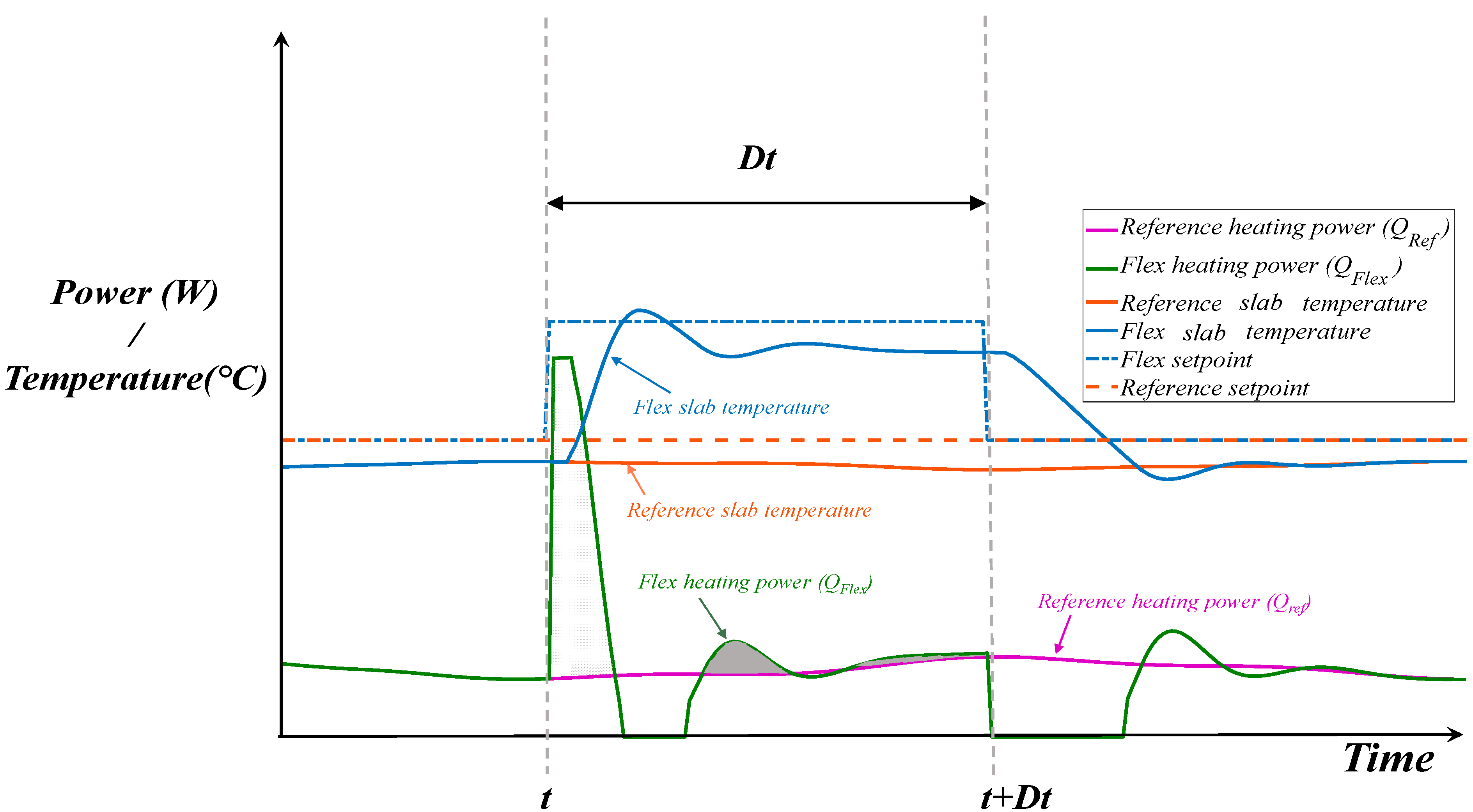
A building energy flexibility index (BEFI) is defined by Athienitis et al. [
44] as the average amount of power (kW) that can be increased or decreased relative to a reference power profile (
Qref, the “as-usual operation”) by the building during a certain period of time (
Dt):
The schematic below in
Figure 1 illustrates the BEFI concept. The grey area during the period
Dt is the numerator of Equation (1) and shows the difference between the flexible and the reference heating loads.
The BEFI could be predicted continuously with a certain accuracy/uncertainty depending on the configuration and duration length. Generally, the shorter the duration, the less the uncertainty is expected. Another factor to consider is the time of activation. For some grid needs, activation time must be within seconds and must be totally autonomous. For others, it can be different and may rely on communication protocols, but once the signal is received by the building, BAS response must be automated. Then, for some others, the need may be planned half a day in advance and the building can be designed and operated to maximize its flexibility during the period of need with potential significant financial benefits in terms of reduced operational costs. In this paper, the BEFI is calculated with dynamic tariffs and a floor heating system.
3. Modeling of Thermal Zones with Radiant Floor Systems
The modeling approach used for this study is based on the low-order lumped-parameter thermal network models which have been shown to be practical for control studies and especially model predictive control [
33,
45]. This approach is generally valid when Biot number is less than 0.1. In this approach the thermal mass under consideration (radiant floor concrete slab) is discretized into a number of control volumes. Each of the discretized control volumes is represented by a node and considered to be isothermal. Each of the nodes, has a lumped thermal capacitance connected to it and thermal conductances connecting it to adjacent nodes. Considering the time interval p and time step Δ
t, the general form of the explicit finite-difference model for the nodes with a lumped thermal capacitance can be stated as
where
Ti,p represents the temperature of node “i” at time step “p”,
Tj,p represents temperature of node “j” at time step “p”,
Ci is the thermal capacitance of node “i”,
Ri,j is the thermal resistance between nodes i and j and
Qi is the heat source at node i.
A model with fewer parameters facilitates setting up the initial conditions which is a key parameter for control studies [
33]. When the details of the construction are not known, a low order grey box modelling approach is practical and can be developed and calibrated by means of real time data from the building. The models must be accurate enough to provide reliable information but also flexible enough for quick and computationally efficient decision-making [
46,
47], especially in reaction to electric grid’s short notices on the change of the price signals.
An important part of a model for zones with radiant floor heating system is the radiative and convective heat transfer which are naturally nonlinear processes. However, the respective heat transfer coefficients are typically linearized so that the system energy balance equations can be solved with linear algebra techniques and represented with a linear thermal network. In the case of radiant floor heating, this linearization generally introduces less error for the for long-wave radiation heat transfer (
hr) than the convection heat exchange between the radiant floor surface and room air (
hcf) [
48]. For example, in the case of radiant floor heating where usually the floor is hotter than the air and the heat flow is upward
hcf is in the order of 3 W/(m
2K) while for a cold floor and warmer air it is in the order of 1 W/(m
2K). For heat flow upwards,
hcf can be calculated as [
49]:
where
Tfloor is the floor surface temperature and
Tair is the zone air temperature.
Therefore, usually certain amount of calibration for the convection heat exchange between the radiant floor and room air is required for a model especially when considering the low order models.
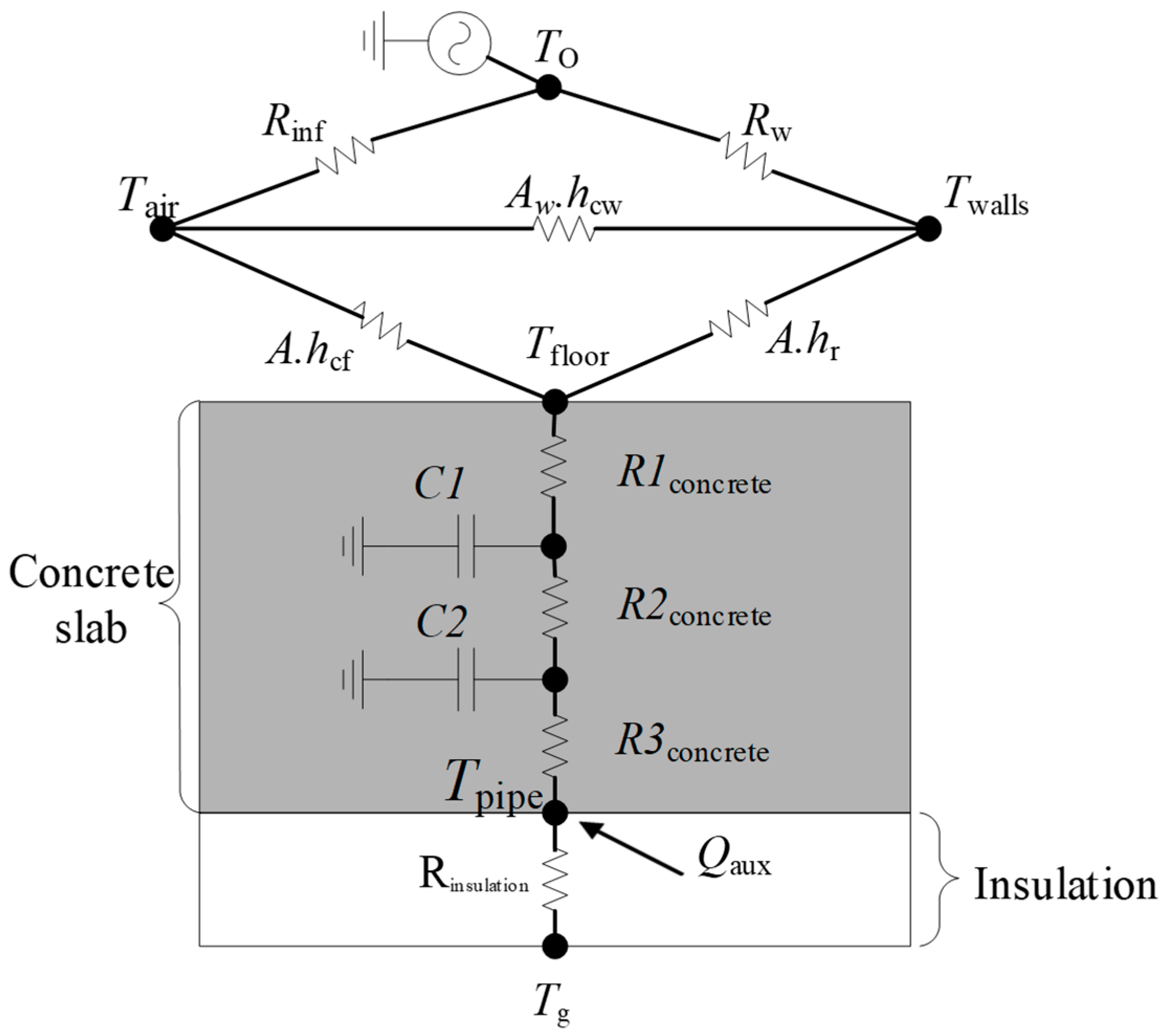
It is demonstrated in the following section, that a well calibrated second-order model, for which the thermal network is shown in
Figure 2, can accurately capture the most important thermal dynamics of a zone with a radiant floor heating system.
Figure 2 also shows the boundary conditions for the model.
Tg is the ground temperature,
hc and
hr are the convective and radiative heat transfer coefficients, respectively, and
Rinf is the infiltration thermal resistance.
In the above thermal network for the case study (Perimeter Zone Test Cell (PZTC)), the hydronic pipes are located at the bottom of the slab and there is a large thermal mass above the pipes that causes significant thermal lag. There can be cases where pipes are placed in the middle of the slab in which case the thermal dynamics will be different. There can also be a case where the location of the pipes is not exactly known, and data from the building automation system can be utilized to calibrate the model.
4. Case Study: Perimeter Zone Test Cell (PZTC)
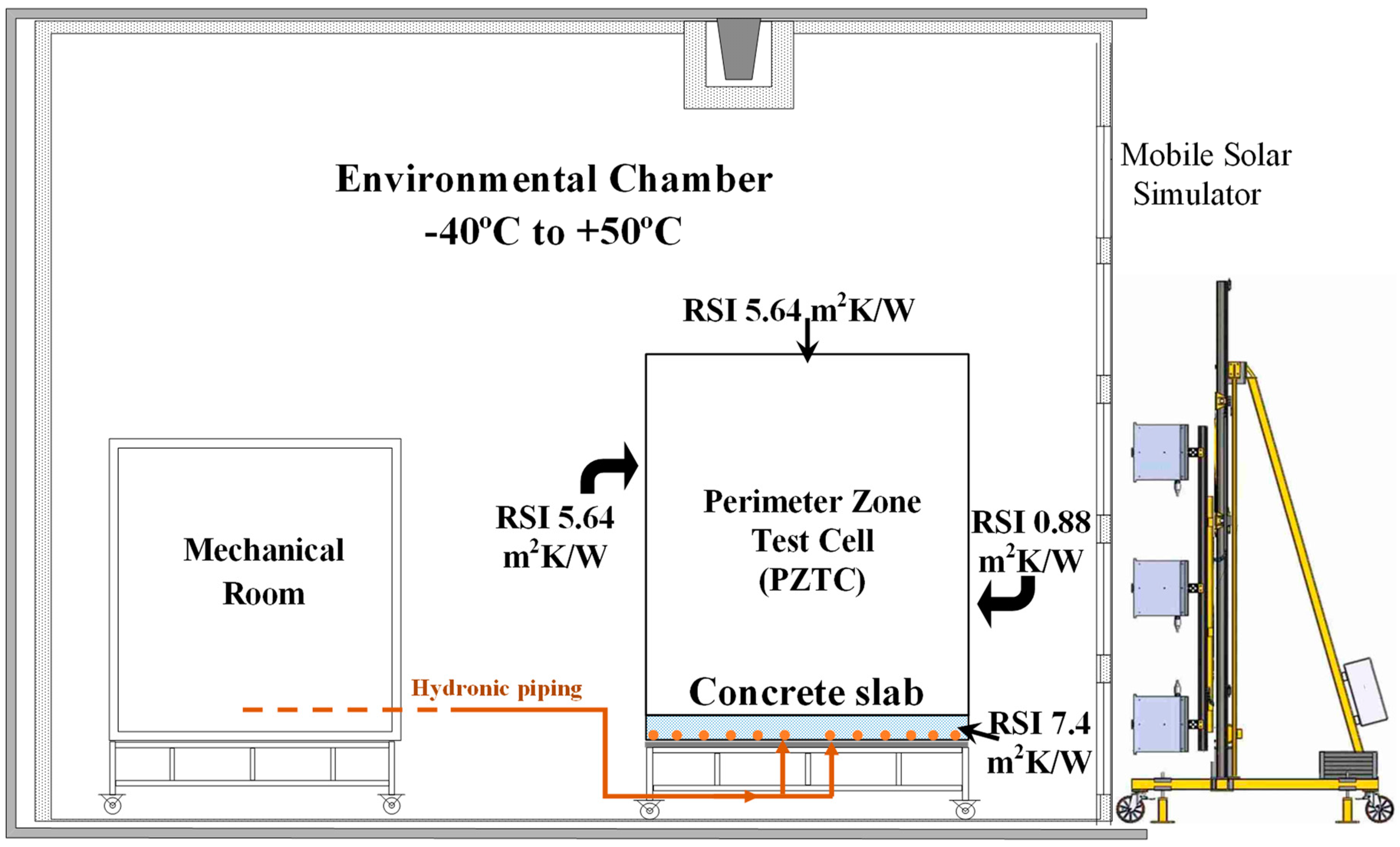
The Solar Simulator-Environmental Chamber (SSEC) laboratory is an experimental facility located at Concordia University in downtown Montreal, Canada. This facility allows accurate and repeatable testing of solar systems and advanced building envelopes under standard test conditions with simulated solar radiation and indoor plus outdoor conditions. The temperature test range of the environmental chamber is −40 °C to +50 °C. Two solar simulators (large-scale and mobile) are designed to emulate solar radiation to test solar systems such as PV and PV/T modules, solar air collectors, solar water collectors and building-integrated solar systems.
The perimeter zone test cell (PZTC) (case study) is a 3 m × 3 m × 3 m room placed inside the solar simulator/environmental chamber laboratory and it contains a radiant floor heating/cooling system. The side and back walls and ceiling consists of 10 cm of insulation with thermal resistance of 5.64 m
2K/W. The front wall is a photovoltaic/thermal solar test façade with 0.88 m
2K/W thermal resistance which was not in operation during the experiment. The floor is made of an approximately 8 cm thick concrete slab, with the piping at the bottom of the concrete and insulation of 7.4 m
2K/W under the slab. Thermal properties of the concrete are shown in
Table 1.
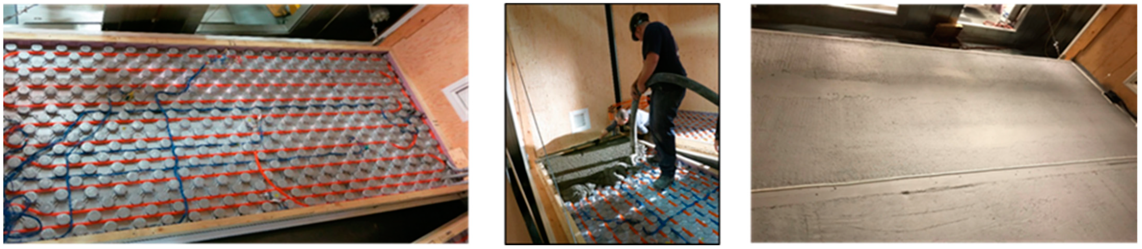
The pipes of the radiant floor system are made of conventional cross-linked polyethylene (PEX) and have an external diameter of 1.75 cm. The pipes are installed in a foam matrix of insulating material that also facilitates keeping them in place. The pipes are spaced at 15 cm.
Figure 3 shows the piping configuration of the radiant floor before the concrete was poured (left), during pouring of concrete and final look of the radiant floor slab (right).
A mechanical room provides controlled flow rate of the fluid (propylene-glycol and water mixture) for the radiant floor. The schematic of the environmental chamber and PZTC is shown in
Figure 4.
A second-order model, for which the thermal network was shown in
Figure 2, was developed for the PZTC (Bi ≈ 0.065 < 0.1). The floor convective heat transfer can vary significantly depending on the temperature difference between the floor surface temperature and the air in the zone. Therefore, an objective function is defined to find the effective values of
hcf so that the floor surface temperature calculated from the simulations (
Tfloor, simulated) matches with experiment (
Tfloor, measured) as accurately as possible. Therefore, the objective function is defined as
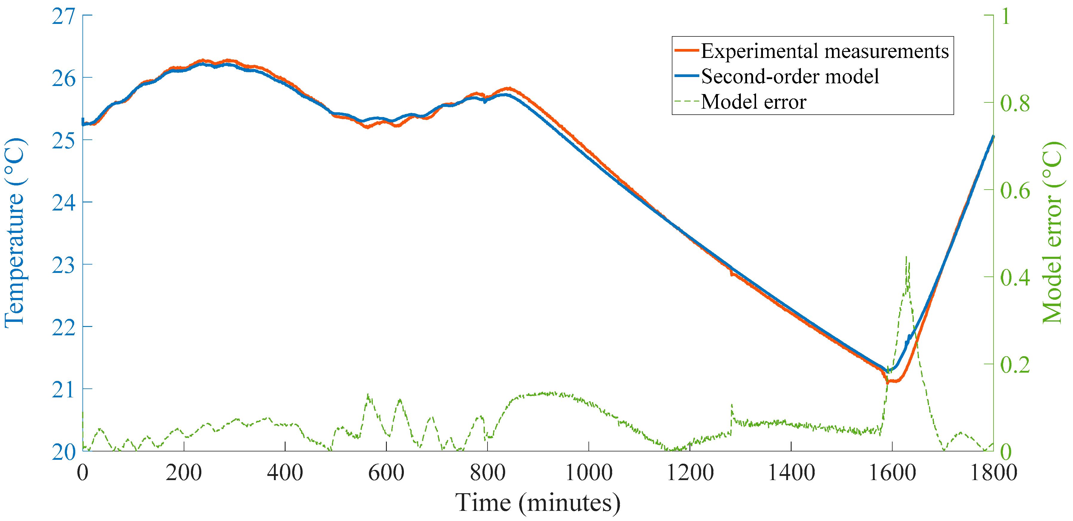
Optimization was done in MATLAB using fmincon function which uses the simplex algorithm. The optimization result is shown in
Figure 5. As observed, a well calibrated second-order model, for which the thermal network shown in
Figure 2, can capture thermal dynamics of a zone that contains radiant floor heating system with a good accuracy and the maximum error between the model and the measurements is about 0.45 °C. However, for the majority of the time the model error is less than 0.1 °C.
This validated model is used in the following sections to study optimal control strategies while dealing with different price signals from the grid. The strategies to deal with the various penalty signals presented in the following sections of this paper are divided into two main categories which are: 1. Predictive strategies with short notice in the order of 10 to 15 mins; 2. Predictive strategies with a prediction horizon of about 1–2 days.
It should be noted that in Quebec two peak demand periods are observed in a day during the heating season which are typically in the morning from 6 to 9 a.m. and in the evening from 4 to 8 p.m. Therefore, the price of the electricity can be different and higher during these periods compared to other times of the day as part of a potential dynamic tariff structure intended to motivate reduced demand for electricity during these periods. The price signals that are assumed and utilized in the following sections are created based on those typical peak demand periods in Quebec.
5. Control Strategies with a Short Notice
In this section thermal response of the radiant floor in reaction to a sudden change in the grid price signal is presented. The control of the radiant floor heating is based on the floor surface temperature since it provides a much smoother heating load profile due to the thermal mass of the floor compared to controlling the zone air temperature which has a very low thermal capacity and hence it causes lots of fluctuations in the heating load. The heating is controlled through proportional control as
where
Tsp = floor surface temperature setpoint,
Tfloor = floor surface temperature, and
Kp is the proportional constant equal to 900 W/°C. The maximum heating output is limited to the size of the system which is 2.7 kW.
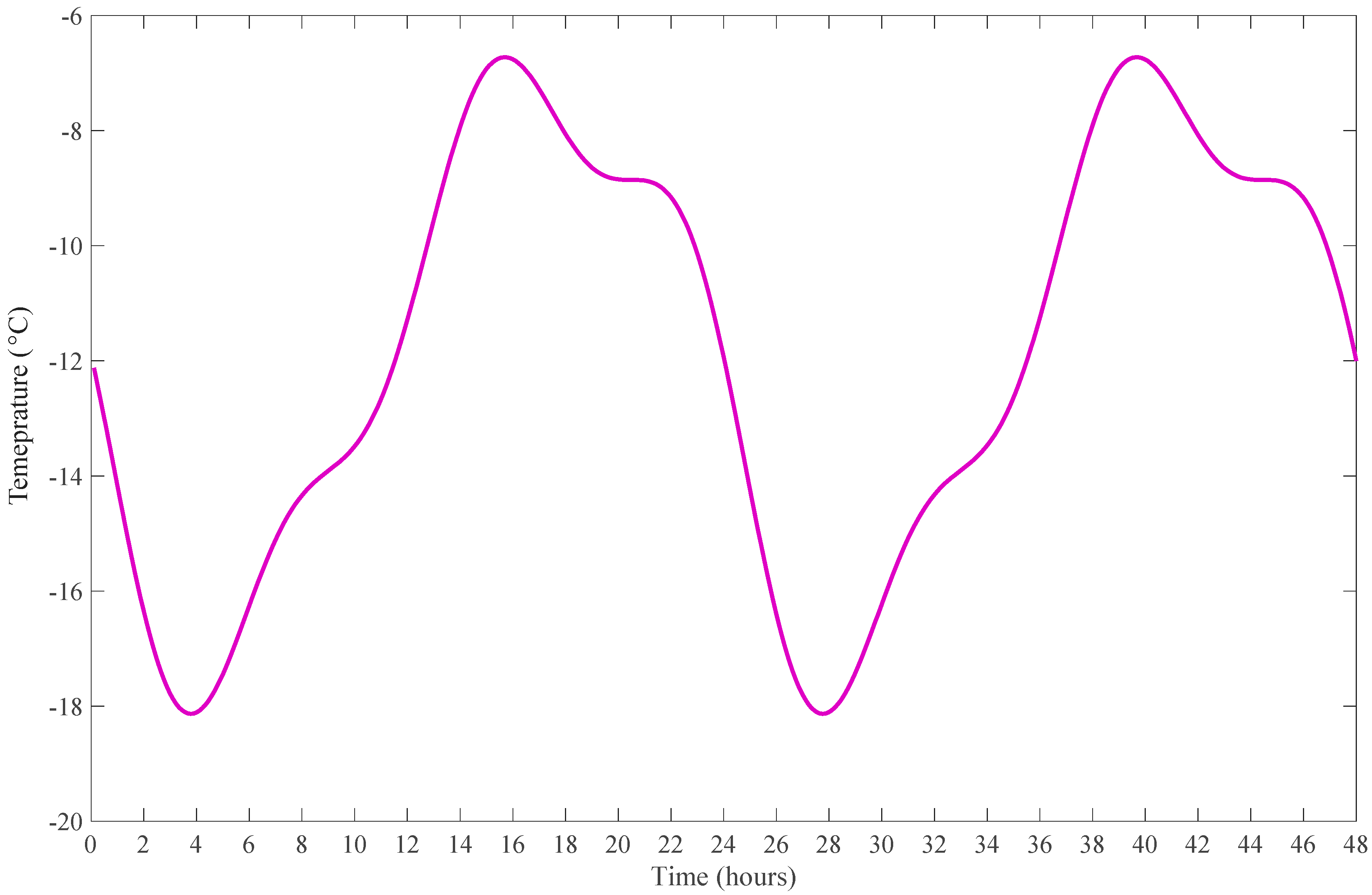
The ambient temperature profile considered is shown in
Figure 6. The ambient temperature changes between −7 °C and −18 °C with the mean value of about −12 °C—a relatively cold day in Quebec when high demand for electric space heating is expected.
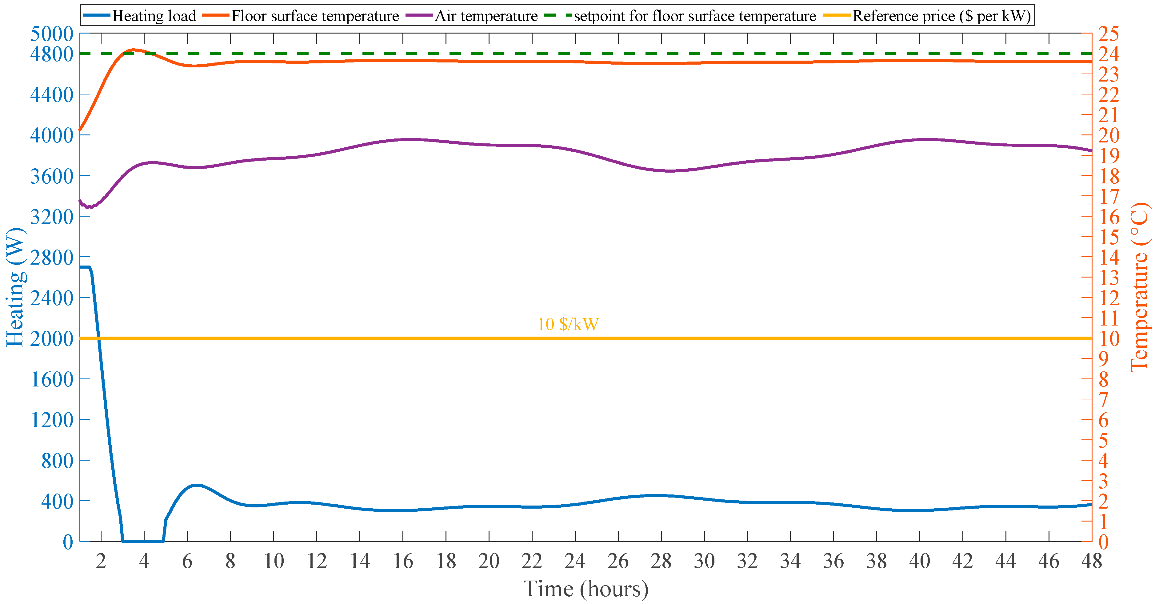
Figure 7 shows the heating load, floor surface temperature and zone air temperature for maintaining a constant floor surface temperature of 24 °C which is considered the reference surface temperature here. The results shown in
Figure 5 is for a day when the electricity price remains constant for the whole day at the reference value which is assumed to be
$10 per kW for power.
As can be observed from
Figure 7, when the floor surface temperature is kept around 24 °C, the zone air temperature stays between 18 °C and 20 °C which is within the typical indoor air temperature comfort range (18–24 °C) for occupants [
50] and the operative temperature also stays within the same range.
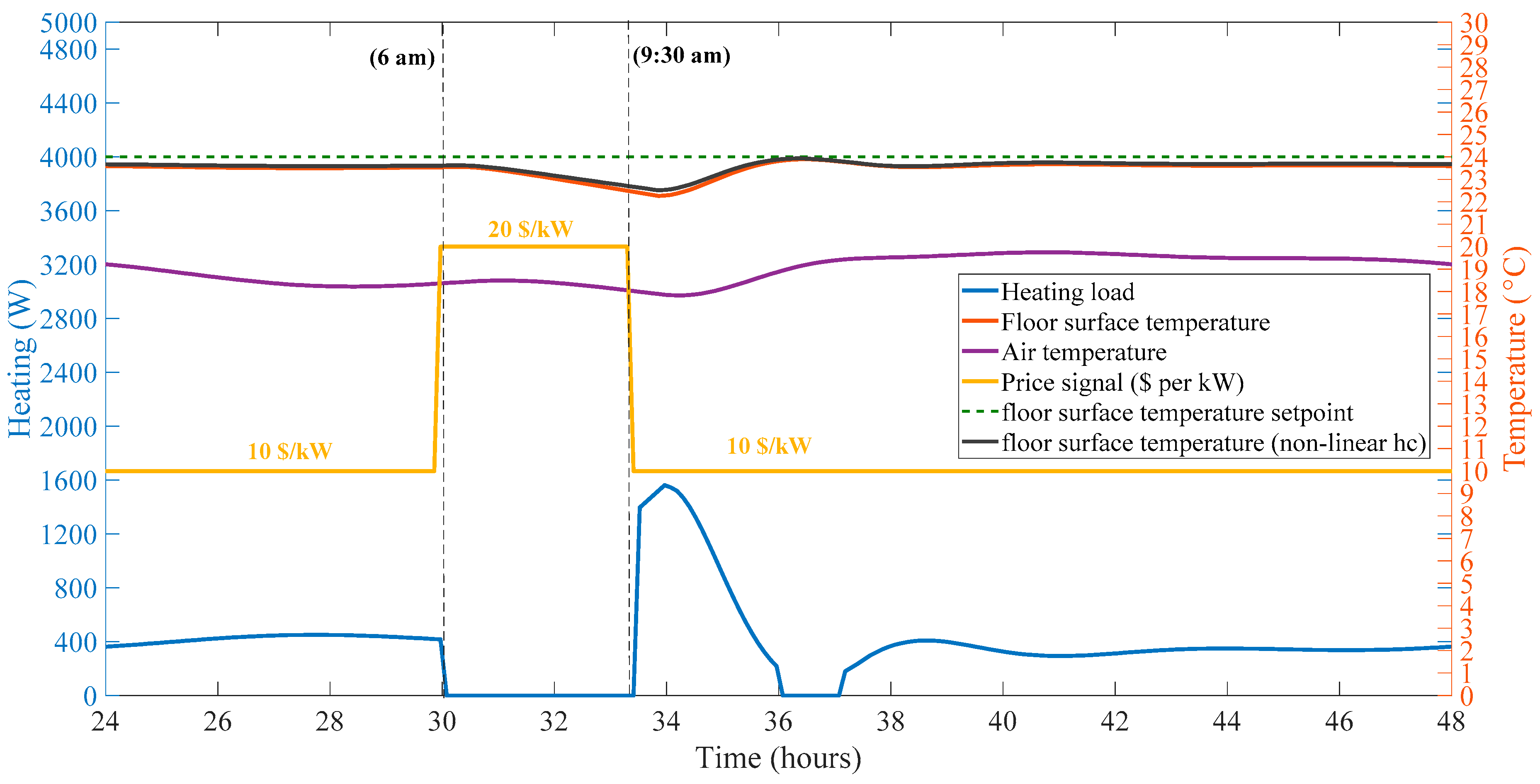
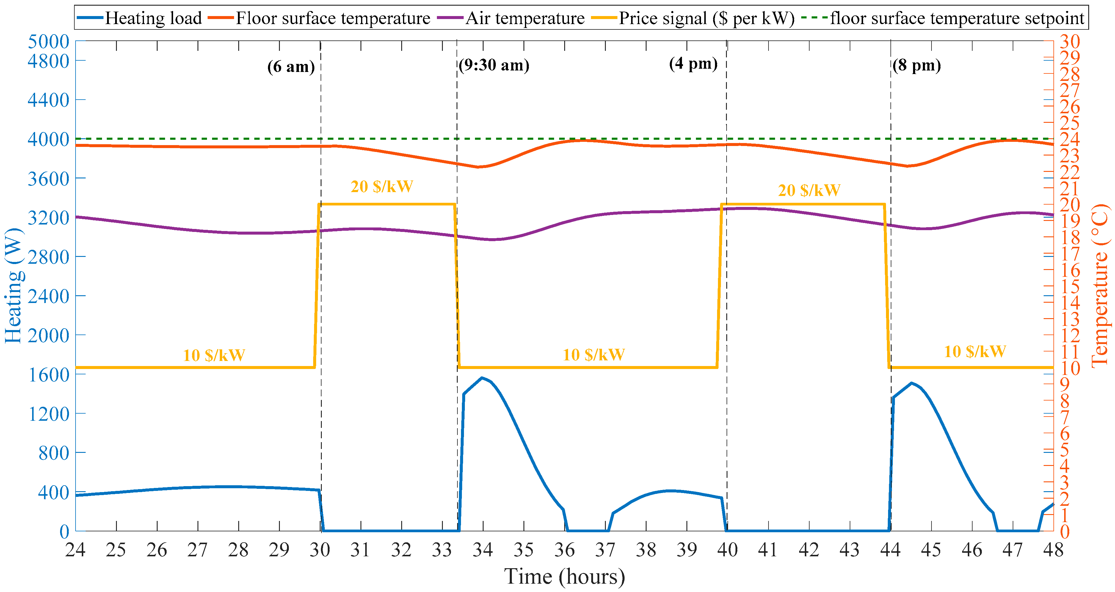
Figure 8 shows the short-notice predictive (almost reactive) behavior to sudden increase, from 10
$/kW to 20
$/kW, in the price signal for a period of 3.5 h (hours between 30 and 33.5) which is the typical morning peak demand period in Quebec (6–9 a.m.). It is assumed that the price of energy (kWh) is constant and only the power (kW) price is changing. The simplest strategy to deal with this sudden increase in the price signal is to turn off the heating system. It can be observed that due to shutdown of the heating system during that the period, the floor surface temperature (red line) falls to 22.2 °C and air temperature (purple line) to 18 °C. Considering the typical comfort boundaries of 18–24 °C for the zone air temperature, the air temperature is at the lower threshold of the comfort boundary. It can be calculated that the BEFI would be roughly about 400 W for 3.5 h. The floor surface temperature is also shown for the case with non-linear convective heat transfer coefficient between floor surface and air temperature (
hcf). As observed, there is no significant difference between the two curves, thus confirming that assuming a linear convective coefficient is an acceptable approximation.
Figure 9 shows another increase in the price signal during the evening on the same day. This second increase is during the evening peak demand hours (4–8 p.m.) in Quebec during winter. As observed, since the second increase event happens when the zone air temperature was higher compared to the first event and generally the system was at a higher state of charge, the air temperature drops to 18.5 °C at lowest and the building can offer the average BEFI of 400 W for 4 h during this period. The operative temperature stays between 19.5 °C and 21 °C.
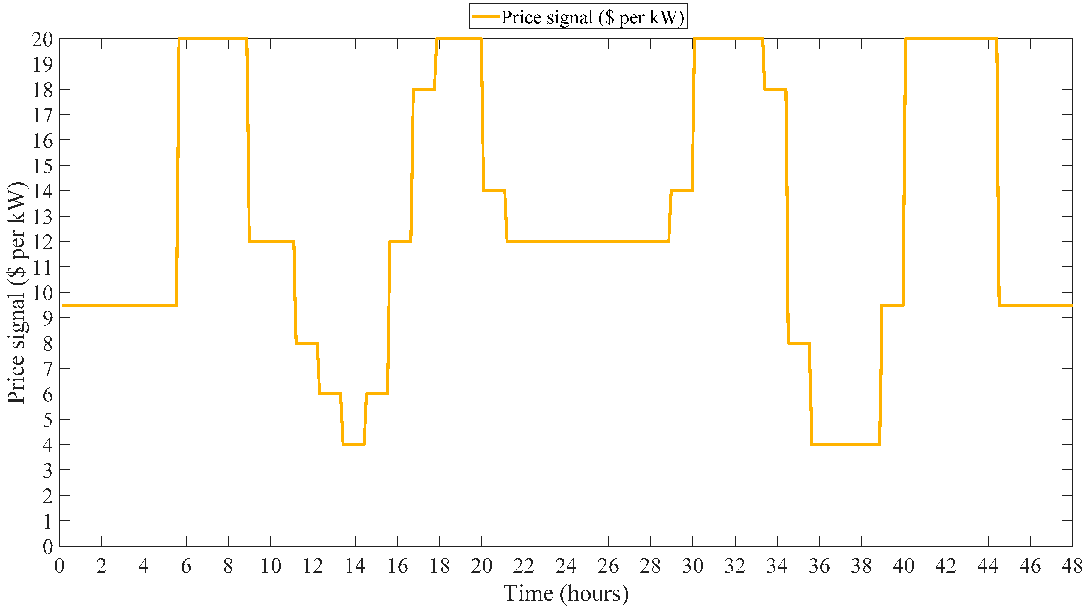
The intermittent nature of renewable energy sources increases the necessity for backup power to deal with the unexpected swings in power production. Therefore, change in the price signal can be more frequent and the price signal from the grid can vary every hour during the day depending on the availability of electricity from renewable energy sources, weather conditions, emergency events, etc. For example, the dynamic price signal for the following 48 h may look like the profile shown in
Figure 10. As can be observed from
Figure 10, the price signal is changing frequently during the day and if we consider the
$10 per kW as the normal, reference operating price signal, there are some periods with price signals higher, as well as lower than the reference.
It should be noted that a short notice (10–15 min or shorter) of a price change from the grid can also be received. The following control strategy is presented for these situations. First let us categorize the upcoming hour price signal into two categories:
- 1.
Price signal lower than the normal reference operating price signal that is: P(t) < Preference
In this case since the price signal is lower than reference then we can just keep the heating control as usual and operating in the reference case (
Qaux,ref) for which the details were explained in equation (5). Therefore, the heating during the low-price period,
Qaux,low-price, is inserted as
- 2.
Price signals higher than the normal reference operating price signal: P(t) > Preference
In this case the strategy will be to keep the floor surface temperature at 24 °C; however, the heating load will be a fraction of the reference heating and this fraction gets smaller as the price increases. Therefore, the strategy is defined as
where
Preference is the reference price and
P(
t) is the price at time t.
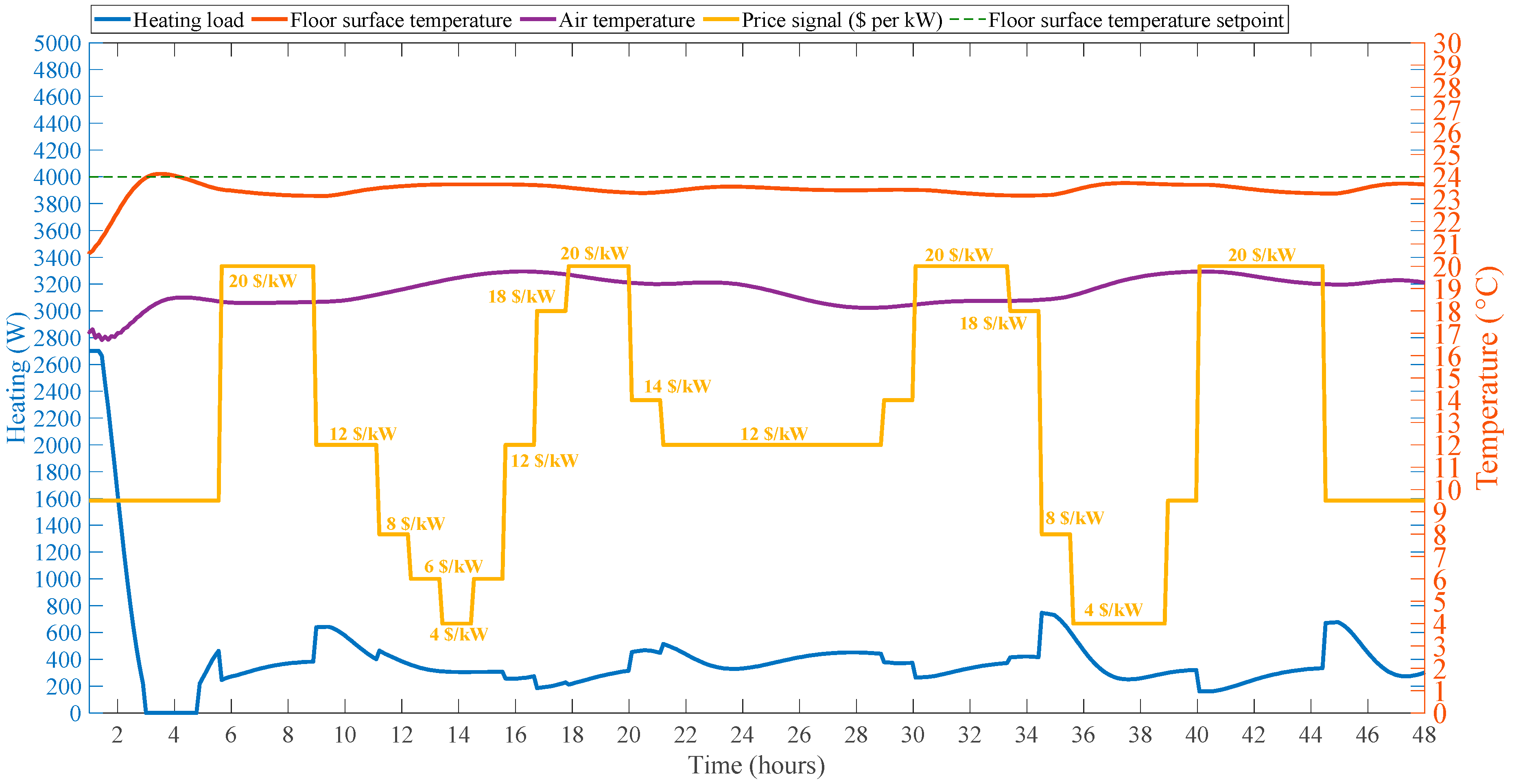
Figure 11 shows the application of this strategy to the thermal zone:
As can be observed, during the high price signal periods, whenever necessary, the heating load was turned on as a fraction of the reference heating load to keep the floor surface temperature near the setpoint hence reducing the amount of heating power and reducing the cost.
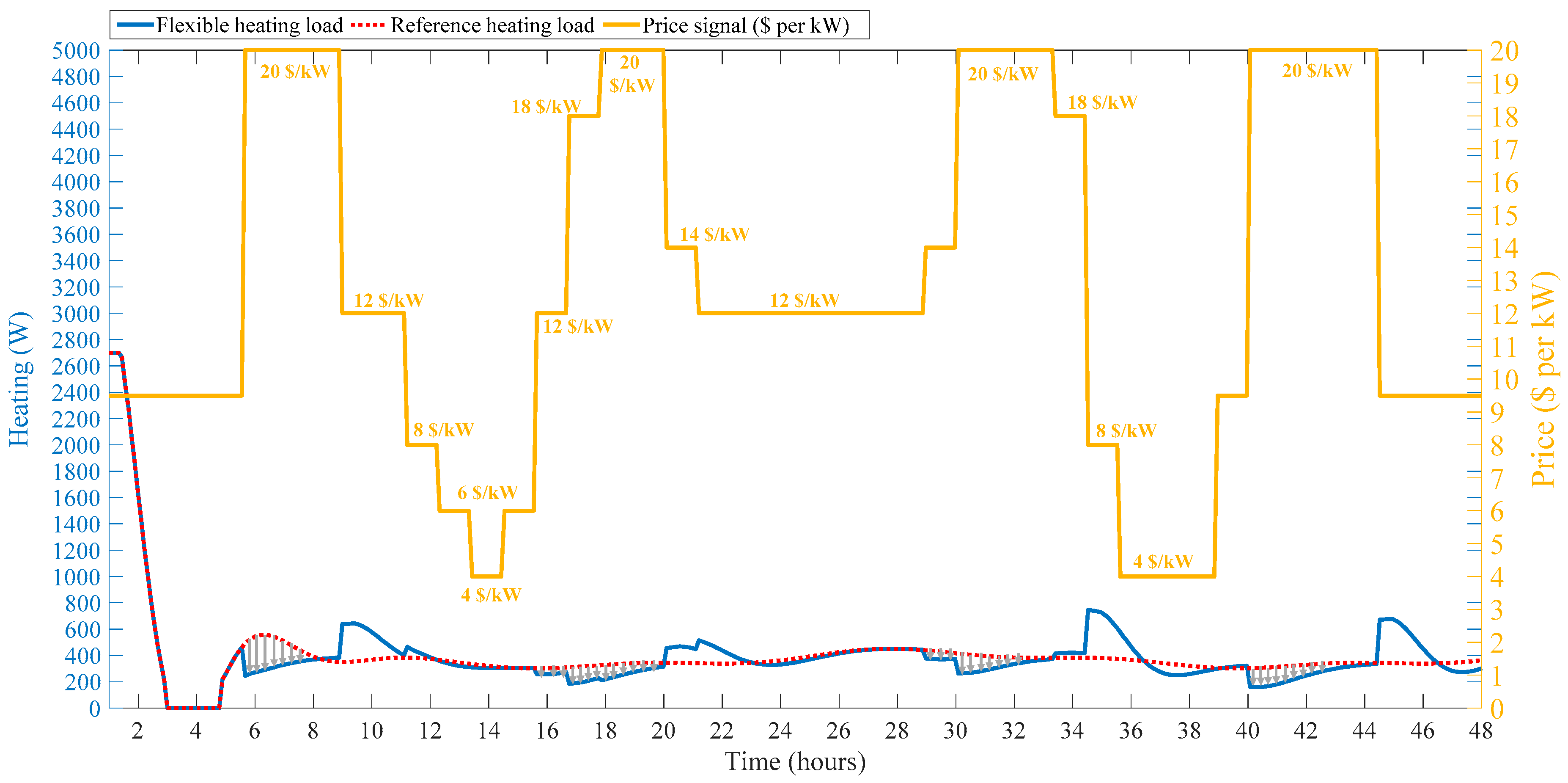
Figure 12 shows the comparison between the reference heating load and the flexible heating load from the strategy above. It can be observed how the above strategy decreases the heating load during the high price periods. As mentioned earlier, BEFI is the amount of power (W) that the building can reduce (or increase) during certain periods of time. Therefore, BEFI during high price signal is the difference between the two curves which is shown by the area covered with the grey arrows.
6. Predictive control strategies with longer prediction horizons
When the prediction of the upcoming days for weather as well the grid price signals are available, the system can be operated in order to minimize the power and/or energy consumption during the high price signal period. In this section the predictive strategies for the price signals given in the previous sections are presented.
Here, the aim is to find a setpoint for the floor surface temperature proportional controller so that the surface temperature stays within the comfort range with 29 °C as maximum based on the ASHRAE standard [
50]. The objective function is defined as
where
Psig is the value of the price signal at every time step. Considering the above range for the floor surface temperature, the operative temperature (T
op) stays between 19 °C and 25 °C. Optimization was done in MATLAB using fmincon function which uses the simplex algorithm.
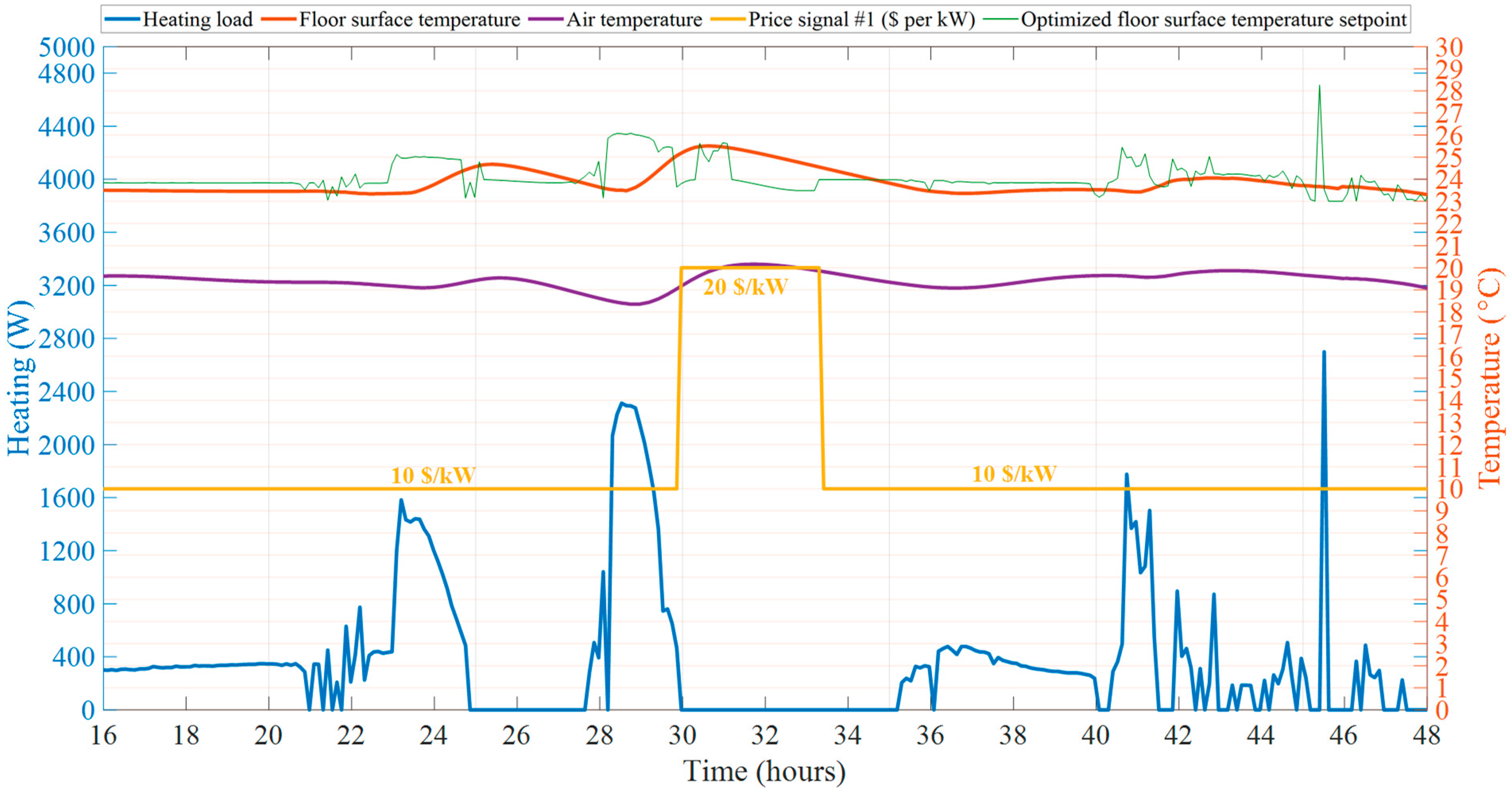
Figure 13 shows the results for the first price signal. As observed, the optimized floor surface temperature setpoint modulates the heating load of the floor in a way to keep the floor surface temperature very close to the minimum of 23 °C during the periods with reference price signal but as we get closer to the high price signal period, it starts preheating the floor slab by increasing the setpoint as high as 26 °C. Therefore, as observed, the heating load is zero during the high price period. The cost for whole period is
$18.60. Now if no optimization was performed and the reference strategy (
Figure 7) was used without considering the change in the price, then the total cost would be
$20.70. Therefore, a decrease of more than 10% in the cost is observed.
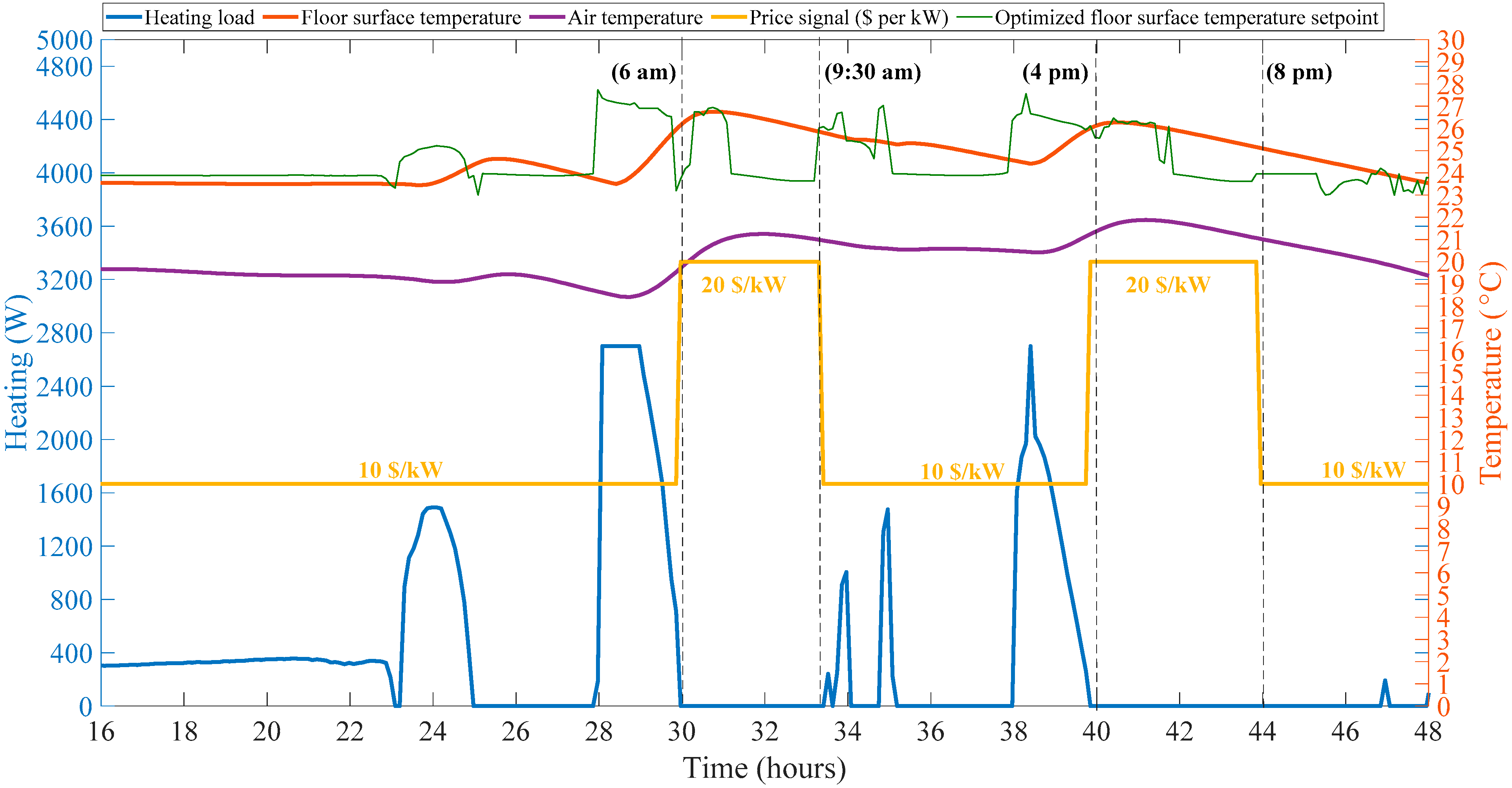
Next, if another price signal was in the forecast in which two periods of high price are expected during the next 48 h, then a new setpoint found from the optimization is applied as shown in
Figure 14.
As can be observed from both
Figure 13 and
Figure 14, the setpoint performs in such a way that the zone is heated up until just before the high price periods and then the setpoint is relatively low during that period so that due the thermal mass of the radiant floor concrete slab, the surface temperature does not drop below that setpoint and therefore, no heating is needed. The cost for the whole period is about
$19, and compared to using reference strategy (cost =
$22), a decrease of 13.63% in the cost is observed.
There can be more complicated price signals in the forecast as well.
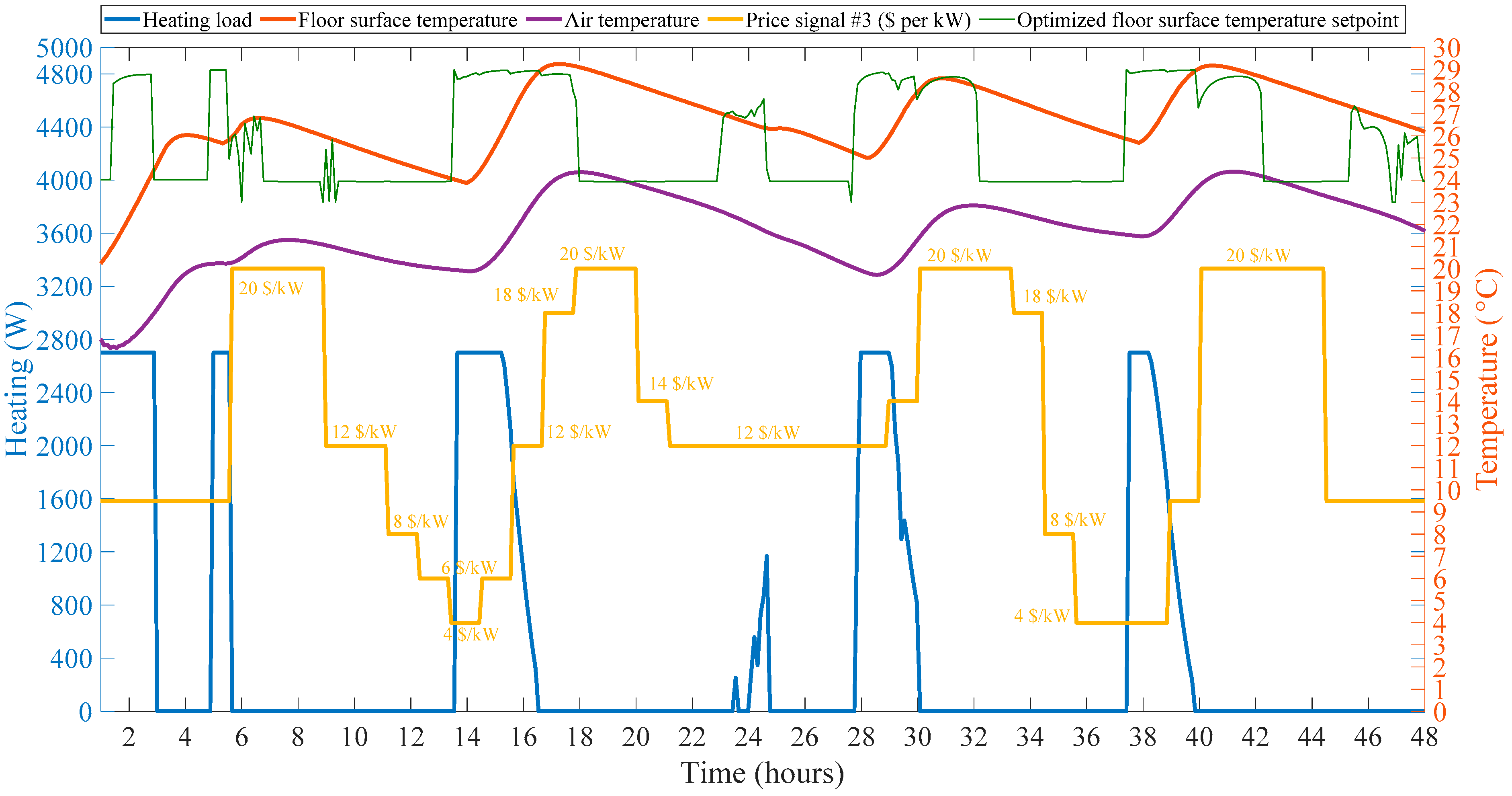
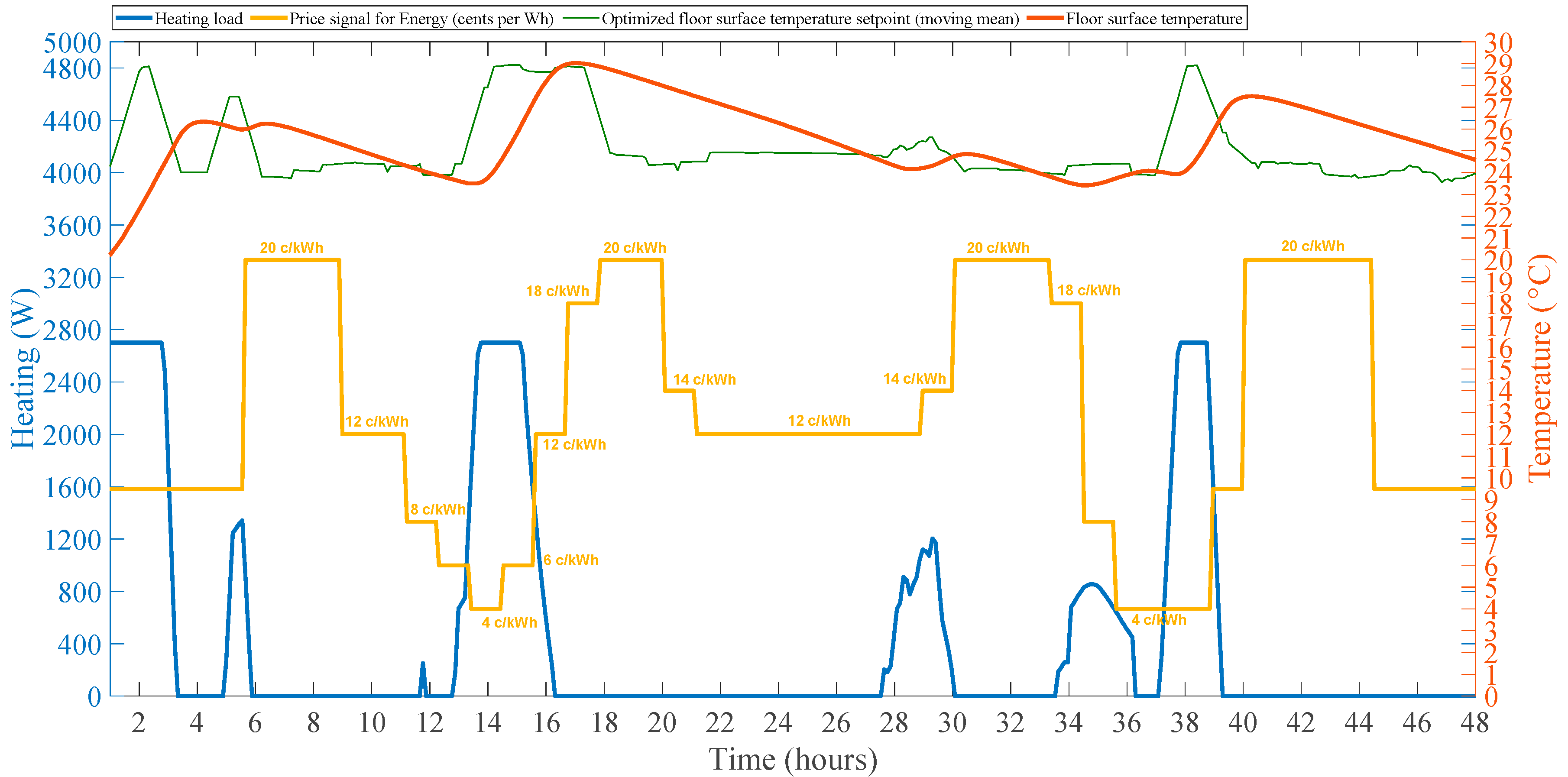
Figure 15 shows the predictive strategy for the price signal that was introduced in the previous section which changes almost every hour. Here, this price signal is known the day before from the forecast.
As can be observed from
Figure 15, the building is heated up during the low-price period (until around 6 a.m.) and the setpoint is increased to the maximum upper threshold for floor surface temperature which is 29 °C. Then, after 6 a.m., there is no heating during the peak demand period (6–9 a.m.) and the warm slab thermal mass lets the heating be turned off until hour 13. Then, the setpoint is again increased to 29 °C to preheat the building and in order to minimize the heating during the afternoon peak demand hours (4–8 p.m.). A similar trend is observed during the next day as well. The total cost with the optimized setpoint is
$18.80 compared to
$24.12 with the reference strategy, resulting in a decrease of 22% in cost.
Emergency and Non-Predicted Change in the Price Signal
Contingency or operating reserve is the amount of power that utility may call when needed to face the loss of a generation unit or other unexpected load balance [
51]. This reserve needs to be available typically within a ten-minute notification time, for a duration of one hour. Therefore, the building automation system or smart thermostat should be able to quantify the amount of power that it can decrease from its current consumption profile for the following hour.
Figure 11,
Figure 12 and
Figure 13 demonstrate the strategy when prediction of the weather as well as the price signal is available.
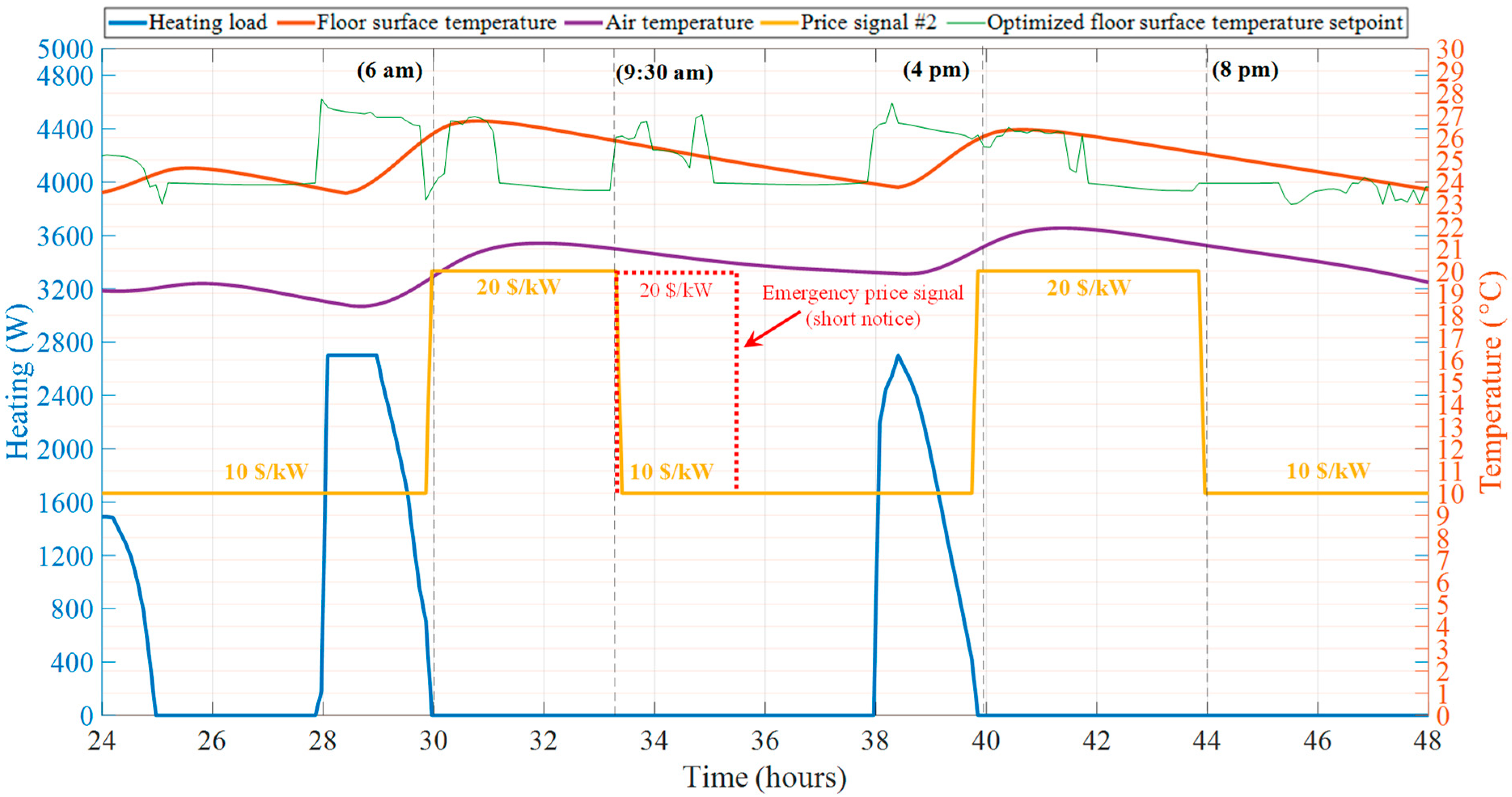
Figure 16 shows the BEFI during a contingency/emergency event when the original predictive strategy before this event was based on the price signal #2 (
Figure 14).
As observed, there is a sudden unexpected increase in the price signal between hours 33.5 and 35.5 (9:30–11:30 a.m.), and therefore the heating was turned off immediately. As shown in
Figure 16 turning off the heating during that period has little impact on the floor surface and air temperatures. The BEFI which is the amount of power that is reduced compared to the reference case (
Figure 14) and is calculated on average as, BEFI = 270 W.
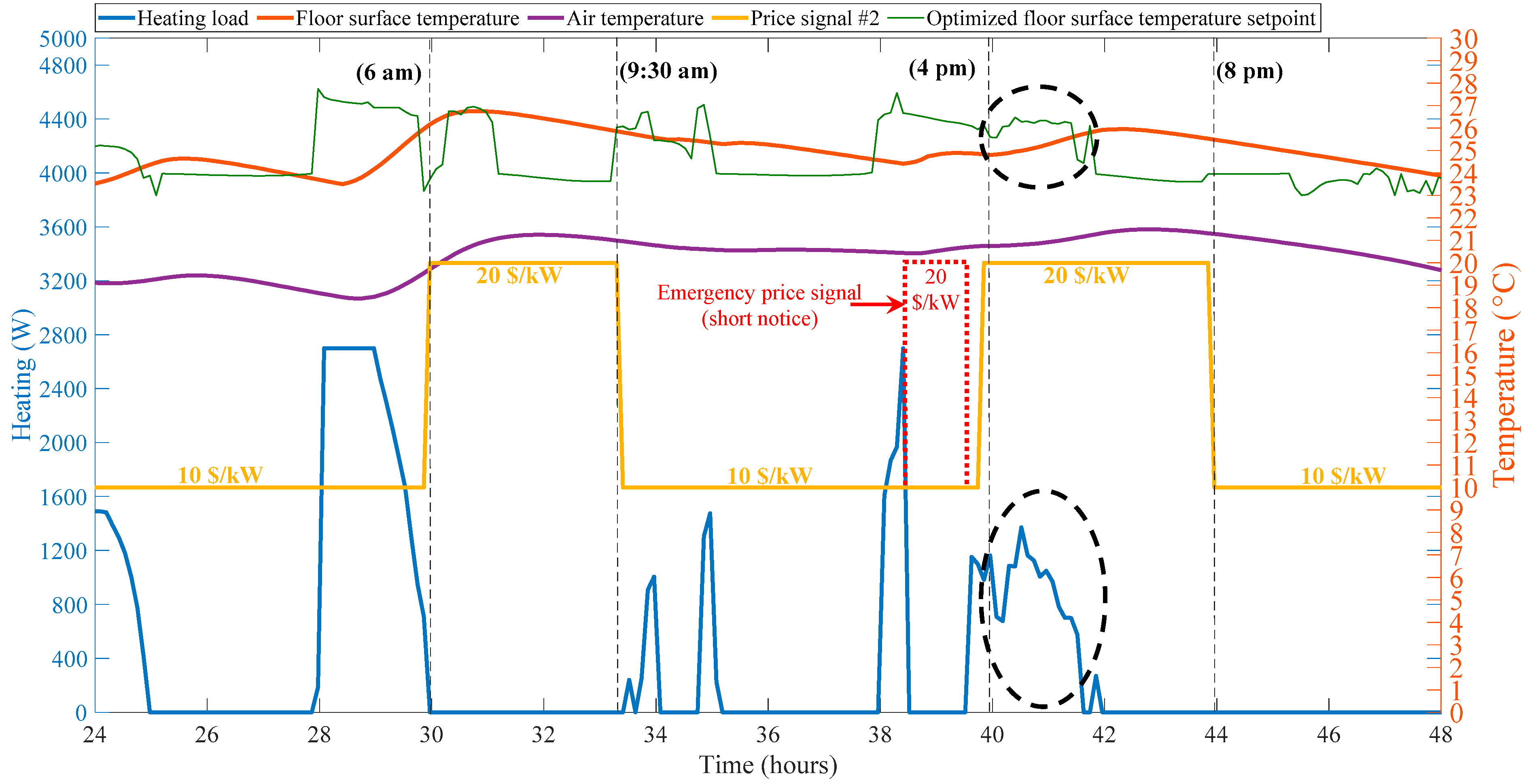
The timing of the unexpected change in the price signal is also particularly important. For example, if the unexpected change happens in a different hour that is closer to the period with a high price, then it could be more challenging to deal with this sudden change. As shown in
Figure 17, if the sudden increase in price signal happens between hours 38.5 and 39.5, then the controller which is acting based on the predictions would not have enough time to follow back the optimized setpoint profile and as the result, some heating is observed during the predicted high price signal period as shown in
Figure 17 with black dashed circles. However, as can be observed from
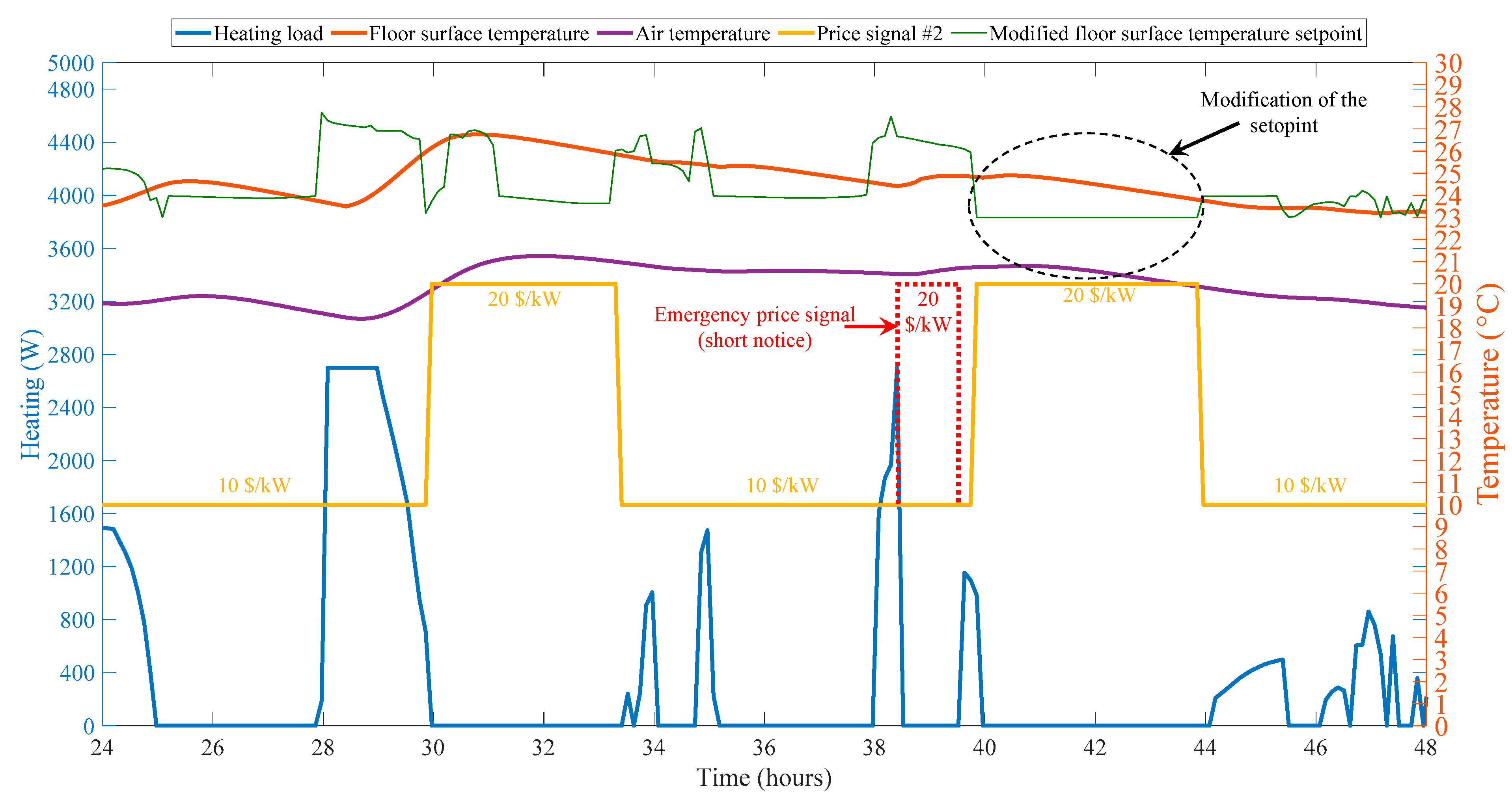
Figure 17, since the floor surface temperature is already above the lower threshold of 23 °C, there is no need for heating. Therefore, in this case the setpoint temperature can be modified for the period between 40 and 44 h and put at the lower threshold of 23 °C. This modification will enable zero power consumption during that period as shown in
Figure 18.
7. Dynamic Pricing of Energy
There are certain situations in which the dynamic pricing is explicitly mentioned for energy consumption (kWh) instead of power (kW). In this case the optimization must be done for energy and the cost for energy (kWh) is minimized instead of power (kW). The unit of the price signal will be cents per kWh (ȼ/kWh).
Figure 19 shows the results.
As observed from
Figure 19, the heating works in a similar way to when it was used to minimize the power consumption. The moving mean of the setpoint profile obtained from the optimization is used since the optimized setpoint contains lots of spikes in the temperature which consequently causes spikes in the heating loads and much on/off cycling which is not practical. Therefore, as can be observed, when minimizing the cost of power, the cost of energy is also minimized.
8. Conclusions
The major contributions of this article can be listed as 1. a methodology to develop low-order models for zones with high-mass radiant floor heating systems; 2. a method for short notice predictive control in response to change in the grid price signal for zones with hydronic floor heating systems; and 3. a method for day-ahead predictive control in response to the change in the grid price signal for the zones with hydronic floor heating systems.
Optimal Control strategies in response to different price signals from the electricity grid with short and long-term predictions were presented to enhance the energy flexibility for a thermal zone equipped with a hydronic floor heating system and significant amount of thermal mass. The flexibility achieved through the floor thermal mass is particularly valuable in interaction with the smart grid to reduce the peak power demand significantly during the critical periods. A methodology to create low order thermal network models was presented and utilized to develop the thermal model of the zone. The model was validated with experimental measurements and subsequently used to study the control strategies. In general, in a building without much knowledge about the details of the construction and zones, a grey-box model similar to the presented second order model can be calibrated in real time by the building automation system to optimize the building performance. Therefore, this modeling methodology can be applied in any location to any zone equipped with a radiant floor heating system.
A method was presented to deal with a short notice price signal that changes every hour during the day and for which the prices can be either higher or lower than the reference operating condition. It was observed that this method can reduce the cost of power consumption while still ensuring the occupant comfort is not violated. Then, an optimization methodology was introduced to minimize the cost function defined based on the predicted price signal for the following days. The optimized floor surface temperature setpoint was found for different price signals to minimize the cost of the heating power (kW) as well as the energy (kWh). It was shown that the strategy can be modified if the price signal prediction would not be as expected and sudden increase in the price happens especially during the critical periods. The full implementation of the developed MPC strategies to a real building will be the next step in the research.
Author Contributions
Conceptualization, A.S.D. and A.K.A.; method-ology, A.S.D. and A.K.A.; software, A.S.D.; validation, A.S.D. and A.K.A., formal analysis, A.S.D. and A.K.A.; investigation, A.S.D.; resources, A.K.A.; data curation, A.S.D.; writing—original draft preparation, A.S.D. and A.K.A.; writing—review and editing, A.S.D. and A.K.A.; visualization, A.S.D. and A.K.A.; supervision, A.K.A.; project administration, A.K.A.; funding acquisition, A.K.A., All authors have read and agreed to the published version of the manuscript.
Funding
This research was funded by NSERC/Hydro-Quebc Industrial Research Chair at Concordia University, grant number IRCPJ 452558-17 and the APC was funded by the same.
Acknowledgments
This research was supported through NSERC/Hydro-Quebec Industrial Research Chair in “Optimized Operation and Energy Efficiency: Towards High Performance Buildings” at Concordia University.
Conflicts of Interest
The authors declare no conflict of interest.
Nomenclature
| Ai | Area of surface represented by node i (m2) |
| BEFI | Building energy flexibility index |
| Ci | Thermal capacitance of node i(J/K) |
| k | Thermal conductivity of materials (W/(m.k)) |
| Kp | Proportional control constant (W/°C) |
| li | Thickness of surface i (m) |
| Psig | Price signal |
| Preference | Reference price signal |
| Qaux | Auxiliary heating source (W) |
| Qi | Source entering node i (W) |
| Qmax | Maximum heating capacity (system size) |
| Qref | Reference heating power profile (W) |
| Ri,j | Thermal resistance between nodes i and j (m2K/W) |
| Rinf | Infiltration thermal resistance (m2W/K) |
| RW | Thermal resistance of walls (m2W/K) |
| Ti | Temperature of node i (°C) |
| Tsp | Air setpoint temperature (°C) |
| To | Outdoor temperature (°C) |
| Tfloor | Floor surface temperature (°C) |
| t | Time |
References
- Boßmann, T.; Staffell, I. The shape of future electricity demand: Exploring load curves in 2050s Germany and Britain. Energy 2015, 90, 1317–1333. [Google Scholar] [CrossRef]
- International Renewable Energy Agency. Global Energy Transformation, A Roadmap to 2050; IRENA: Abu Dhabi, United Arab Emirates, 2018. [Google Scholar]
- Cui, B.; Wang, S.; Yan, C.; Xue, X. Evaluation of a fast power demand response strategy using active and passive building cold storages for smart grid applications. Energy Convers. Manag. 2015, 102, 227–238. [Google Scholar] [CrossRef]
- Xue, X.; Wang, S.; Yan, C.; Cui, B. A fast chiller power demand response control strategy for buildings connected to smart grid. Appl. Energy 2015, 137, 77–87. [Google Scholar] [CrossRef]
- Gao, D.-C.; Sun, Y.; Lu, Y. A robust demand response control of commercial buildings for smart grid under load prediction uncertainty. Energy 2015, 93, 275–283. [Google Scholar] [CrossRef]
- Huang, P.; Xu, T.; Sun, Y. A genetic algorithm based dynamic pricing for improving bi-directional interactions with reduced power imbalance. Energy Build. 2019, 199, 275–286. [Google Scholar] [CrossRef]
- International Energy Agency Photovoltaic Power Systems Programme. Snapshot of Global PV Markets 2020; IEAPPSP: Fribourg, Switzerland, 2020. [Google Scholar]
- Global Wind Energy Council. Global Wind Statistics 2019; GWEC: Brussels, Belgium, 2019. [Google Scholar]
- International Energy Agency. Germany 2020 Energy Policy Review; IEA: Paris, France, 2020. [Google Scholar]
- Danish Energy Agency. The Danish Energy Model: Innovative Efficient and Sustainable; Danish Energy Agency: København, Denmark, 2020. [Google Scholar]
- Clermont, A. Contribution des Batiments Institutionnels dans L’atteinte de L’ind’Ependance Energetique du Quebec et dans la Lutte Contre les Changements Climatiques. Ph.D. Thesis, Universite de Sherbrooke, Sherbrooke, QC, Canada, June 2015. [Google Scholar]
- Morales, M.J.; Conejo, A.J.; Madsen, H.; Pinson, P.; Zugno, M. Integrating Renewables in Electricity Markets: Operational Problems; Springer: Berlin/Heidelberg, Germany, 2013. [Google Scholar]
- Aelenei, D.; Lopes, R.A.; Aelenei, L.; Gonçalves, H. Investigating the potential for energy flexibility in an office building with a vertical BIPV and a PV roof system. Renew. Energy 2019, 137, 189–197. [Google Scholar] [CrossRef]
- Narayanan, S.; Mets, K.; Strobbe, M.; Develder, C. Feasibility of 100% renewable energy-based electricity production for cities with storage and flexibility. Renew. Energy 2019, 134, 689–709. [Google Scholar] [CrossRef]
- Child, M.; Kemfert, C.; Bogdanov, D.; Breyer, C. Flexible electricity generation, grid exchange and storage for the transition to a 100% renewable energy system in Europe. Renew. Energy 2019, 139, 80–101. [Google Scholar] [CrossRef]
- English, J.; Niet, T.; Lyseng, B.; Keller, V.; Palmer-Wilson, K.; Robertson, B.; Wild, P.; Rowe, A. Flexibility requirements and electricity system planning: Assessing inter-regional coordination with large penetrations of variable renewable supplies. Renew. Energy 2020, 145, 2770–2782. [Google Scholar] [CrossRef]
- Lund, P.D.; Lindgren, J.; Mikkola, J.; Salpakari, J. Review of energy system flexibility measures to enable high levels of variable renewable electricity. Renew. Sustain. Energy Rev. 2015, 45, 785–807. [Google Scholar] [CrossRef]
- El Geneidy, R.; Howard, B. Contracted energy flexibility characteristics of communities: Analysis of a control strategy for demand response. Appl. Energy 2020, 263, 114600. [Google Scholar] [CrossRef]
- Finck, C.; Li, R.; Zeiler, W. Optimal control of demand flexibility under real-time pricing for heating systems in buildings: A real-life demonstration. Appl. Energy 2020, 263, 114671. [Google Scholar] [CrossRef]
- Zhou, Y.; Zheng, S. Machine-learning based hybrid demand-side controller for high-rise office buildings with high energy flexibilities. Appl. Energy 2020, 262, 114416. [Google Scholar] [CrossRef]
- Østergaard, J.S.; Marszal-Pomianowska, A.; Lollini, R.; Pasut, W.; Knotzer, A.; Engelmann, P.; Stafford, A.; Reynders, G. IEA EBC Annex 67 Energy Flexible Buildings. Energy Build. 2017, 155, 25–34. [Google Scholar] [CrossRef]
- Reynders, G.; Lopes, R.A.; Marszal-Pomianowska, A.; Aelenei, D.; Martins, J.; Saelens, D. Energy flexible buildings: An evaluation of definitions and quantification methodologies applied to thermal storage. Energy Build. 2018, 166, 372–390. [Google Scholar] [CrossRef]
- Brunner, C.; Deac, G.; Braun, S.; Zöphel, C. The future need for flexibility and the impact of fluctuating renewable power generation. Renew. Energy 2020, 149, 1314–1324. [Google Scholar] [CrossRef]
- Arteconi, A.; Mugnini, A.; Polonara, F. Energy flexible buildings: A methodology for rating the flexibility performance of buildings with electric heating and cooling systems. Appl. Energy 2019, 251, 113387. [Google Scholar] [CrossRef]
- Hu, M.; Xiao, F. Quantifying uncertainty in the aggregate energy flexibility of high-rise residential building clusters considering stochastic occupancy and occupant behavior. Energy 2020, 194, 116838. [Google Scholar] [CrossRef]
- Saberi Derakhtenjani, A.; Athienitis, A.K. A frequency domain transfer function methodology for thermal characterization and design for energy flexibility of zones with radiant systems. Renew. Energy 2020, 163, 1033–1045. [Google Scholar] [CrossRef]
- Mugnini, A.; Coccia, G.; Polonara, F.; Arteconi, A. Performance Assessment of Data-Driven and Physical-Based Models to Predict Building Energy Demand in Model Predictive Controls. Energies 2020, 13, 3125. [Google Scholar] [CrossRef]
- Bahramnia, P.; Rostami, S.M.H.; Wang, J.; Kim, G.-J. Modeling and Controlling of Temperature and Humidity in Building Heating, Ventilating, and Air Conditioning System Using Model Predictive Control. Energies 2019, 12, 4805. [Google Scholar] [CrossRef]
- Ruiz, G.R.; Segarra, E.L.; Bandera, C.F. Model Predictive Control Optimization via Genetic Algorithm Using a Detailed Building Energy Model. Energies 2018, 12, 34. [Google Scholar] [CrossRef]
- Siroký, J.; Oldewurtel, F.; Cigler, J.; Prívara, S. Experimental analysis of model predictive control for an energy efficient building heating system. Appl. Energy 2011, 88, 3079–3087. [Google Scholar] [CrossRef]
- Qin, S.; Badgwell, T. A survey of industrial model predictive control technology. Control Eng. Pract. 2003, 11, 733–764. [Google Scholar] [CrossRef]
- Drgoňa, J.; Arroyo, J.; Figueroa, I.C.; Blum, D.; Arendt, K.; Kim, D.; Ollé, E.P.; Oravec, J.; Wetter, M.; Vrabie, D.L.; et al. All you need to know about model predictive control for buildings. Annu. Rev. Control. 2020, 50, 190–232. [Google Scholar] [CrossRef]
- Candanedo, J.; Dehkordi, V.; Lopez, P. A control-oriented simplified building modeling strategy. In Proceedins of the BS2013: 13th Conference of International Building Performance Simulation Association, Chambéry, France, 26–28 August 2013. [Google Scholar]
- Serale, G.; Fiorentini, M.; Capozzoli, A.; Bernardini, D.; Bemporad, A. Model Predictive Control (MPC) for Enhancing Building and HVAC System Energy Efficiency: Problem Formulation, Applications and Opportunities. Energies 2018, 11, 631. [Google Scholar] [CrossRef]
- Reynders, G.; Diriken, J.; Saelens, D. Quantifying the active demand response potential: Impact of dynamic boundary conditions. In Proceedings of the 12th REHVA World Congress, Aalborg, Denmark, 22–25 May 2016. [Google Scholar]
- Le Dreau, J.; Heiselberg, P. Energy flexibility of residential buildings using short term heat storage in the thermal mass. Energy 2016, 111, 991–1002. [Google Scholar] [CrossRef]
- Foteinaki, K.; Li, R.; Heller, A.; Rode, C. Heating system energy flexibility of low-energy residential buildings. Energy Build. 2018, 180, 95–108. [Google Scholar] [CrossRef]
- Weiß, T.; Fulterer, A.M.; Knotzer, A. Energy flexibility of domestic thermal loads—A building typology approach of the residential building stock in Austria. Adv. Build. Energy Res. 2017, 13, 122–137. [Google Scholar] [CrossRef]
- Niu, J.; Tian, Z.; Lu, Y.; Zhao, H. Flexible dispatch of a building energy system using building thermal storage and battery energy storage. Appl. Energy 2019, 243, 274–287. [Google Scholar] [CrossRef]
- Zhou, Y.; Cao, S. Energy flexibility investigation of advanced grid-responsive energy control strategies with the static battery and electric vehicles: A case study of a high-rise office building in Hong Kong. Energy Convers. Manag. 2019, 199, 111888. [Google Scholar] [CrossRef]
- Junker, R.G.; Azar, A.G.; Lopes, R.A.; Lindberg, K.B.; Reynders, G.; Relan, R.; Madsen, H. Characterizing the energy flexibility of buildings and districts. Appl. Energy 2018, 225, 175–182. [Google Scholar] [CrossRef]
- Hu, M.; Xiao, F.; Jørgensen, J.B.; Li, R. Price-responsive model predictive control of floor heating systems for demand response using building thermal mass. Appl. Therm. Eng. 2019, 153, 316–329. [Google Scholar] [CrossRef]
- Reynders, G. Quantifying the Impact of Building Design on the Potential of Structural Storage for Active Demand Response in Residential Buildings. Ph.D. Thesis, Leuven, Belgium, September 2015. [Google Scholar]
- Athienitis, A.K.; Morovat, N.; Date, J. Development of a dynamic energy flexibility index for buildings and their interaction with smart grids. In Proceedings of the ACEEE 2020 Summer Study on Energy Efficiency in Buildings, Pacific Grove, CA, USA, 17–21 August 2020. [Google Scholar]
- Kim, D.; Braun, J.E. Reduced-order building modeling for application to madel-based predictive control. Proc. SimBuild 2012, 5, 554–561. [Google Scholar]
- Joe, J.; Karava, P.; Hou, X.; Hu, J. Model Predictive Control of a Radiant Floor Cooling System in an Office Space. In Proceedings of the International High-Performance Buildings Conference, West Lafayette, IN, USA, 11–14 July 2016. [Google Scholar]
- Candanedo, J.; Saberi Derakhtenjani, A.; D’Avignon, K.; Athienitis, A.K. A pathway for the derivation of control-oriented models for radiant floor heating applications. In Proceedings of the eSim 2018 10th conference of IBPSA-Canada, Montréal, QC, Canada, 9–10 May 2018; pp. 57–64. [Google Scholar]
- Athienitis, A.K.; O’Brien, W. Modelling, Design and Optimization of Net-Zero Energy Buildings; Wiley Ernst & Sohn: Berlin, Germany, 2015. [Google Scholar]
- ASHRAE. ASHRAE HVAC Applications; ASHRAE: Atlanta, GA, USA, 2017. [Google Scholar]
- ASHRAE. Standard 55: Thermal Environmental Conditions for Human Occupancy; ASHRAE: Atlanta, GA, USA, 2010. [Google Scholar]
- Wang, J.; Wang, X.; Wu, Y. Operating Reserve Model in the Power Market. IEEE Trans. Power Syst. 2005, 20, 223–229. [Google Scholar] [CrossRef]
Figure 1.
Schematic illustration of Building Energy Flexibility Index (BEFI).
Figure 1.
Schematic illustration of Building Energy Flexibility Index (BEFI).
Figure 2.
Second-order model thermal network of floor heating system.
Figure 2.
Second-order model thermal network of floor heating system.
Figure 3.
Radiant floor piping before (left), during (middle) and after (right) pouring the concrete.
Figure 3.
Radiant floor piping before (left), during (middle) and after (right) pouring the concrete.
Figure 4.
Schematic of Solar Simulator-Environmental Chamber (SSEC) with Perimeter Zone Test Cell (PZTC) and radiant floor.
Figure 4.
Schematic of Solar Simulator-Environmental Chamber (SSEC) with Perimeter Zone Test Cell (PZTC) and radiant floor.
Figure 5.
Second-order model versus experimental measurements and model error.
Figure 5.
Second-order model versus experimental measurements and model error.
Figure 6.
Ambient temperature profile.
Figure 6.
Ambient temperature profile.
Figure 7.
Reference conditions and power price for floor surface temperature setpoint of 24 °C.
Figure 7.
Reference conditions and power price for floor surface temperature setpoint of 24 °C.
Figure 8.
Reactive response to sudden increase in the price signal.
Figure 8.
Reactive response to sudden increase in the price signal.
Figure 9.
Reactive responses to sudden increase in the price signal.
Figure 9.
Reactive responses to sudden increase in the price signal.
Figure 10.
Example of dynamic price signal considered.
Figure 10.
Example of dynamic price signal considered.
Figure 11.
Application of the nearly reactive strategy to deal with the changing price signal.
Figure 11.
Application of the nearly reactive strategy to deal with the changing price signal.
Figure 12.
BEFI during high price signal periods.
Figure 12.
BEFI during high price signal periods.
Figure 13.
Predictive strategy for price signal #1.
Figure 13.
Predictive strategy for price signal #1.
Figure 14.
Predictive strategy for price signal #2.
Figure 14.
Predictive strategy for price signal #2.
Figure 15.
Predictive strategy for price signal #3.
Figure 15.
Predictive strategy for price signal #3.
Figure 16.
Unexpected increase in the price signal #2.
Figure 16.
Unexpected increase in the price signal #2.
Figure 17.
Unexpected change in the price signal.
Figure 17.
Unexpected change in the price signal.
Figure 18.
Modified setpoint to correct the heating load.
Figure 18.
Modified setpoint to correct the heating load.
Figure 19.
Predictive strategy for dynamic energy price signal.
Figure 19.
Predictive strategy for dynamic energy price signal.
Table 1.
Thermal properties of concrete.
Table 1.
Thermal properties of concrete.
| Properties | |
|---|
| Thermal conductivity | 1.7 W/(m.K) |
| Specific heat | 800 J/(kg.K) |
| Density | 2010 kg/m3 |
| Publisher’s Note: MDPI stays neutral with regard to jurisdictional claims in published maps and institutional affiliations. |
© 2021 by the authors. Licensee MDPI, Basel, Switzerland. This article is an open access article distributed under the terms and conditions of the Creative Commons Attribution (CC BY) license (http://creativecommons.org/licenses/by/4.0/).


