Article

Coordinated Control of Virtual Power Plants to Improve Power System Short-Term Dynamics

1
Room 157, School of Electrical and Electronic Engineering, University College Dublin, Belfield, D04 V1W8 Dublin, Ireland
2
School of Electrical Engineering, Xinjiang University, Ürümchi 830046, China
3
DIgSILENT GmbH, 72810 Gomaringen, Germany
*
Author to whom correspondence should be addressed.
Energies 2021, 14(4), 1182; https://doi.org/10.3390/en14041182
Submission received: 26 January 2021 / Revised: 11 February 2021 / Accepted: 20 February 2021 / Published: 23 February 2021

Abstract

:
The paper proposes a coordinated frequency control strategy for Virtual Power Plant (VPPs), with the inclusion of Distributed Energy Resource (DERs), e.g., Solar Photo-Voltaic Generation (SPVG), Wind Generator (WG) as well as Energy Storage System (ESS). The objective is to improve the short-term dynamic response of the overall power system. The robustness of the proposed control is evaluated through a Monte Carlo analysis and a detailed modeling of stochastic disturbances of loads, wind speed, and solar irradiance. The impact of communication delays of a variety of realistic communication networks with different bandwidths is also discussed and evaluated. The case study is based on a modified version of the WSCC 9-bus test system with inclusion of a VPP. This is modeled as a distribution network with inclusion of a variety of DERs.

1. Introduction

1.1. Motivation

A Virtual Power Plant (VPP) is obtained by aggregating the capacity of several Distributed Energy Resource (DERs), Energy Storage System (ESS), and dispatchable loads [1]. It operates as a virtual transmission-connected generator in the existing power system [2]. For operation purposes, the active power output of a VPP is scheduled similarly to conventional generators, e.g., through the solution of a daily ahead unit-commitment problem [3]. In transient conditions, e.g., following a contingency, VPPs must provide frequency support [4]. The active power scheduling and the frequency control are generally decoupled due to their different time scales. Instead, this paper proposes to combine these functions by switching to coordinated control of the DERs and ESSs that form the VPP during the contingency.

1.2. Literature Review

The primary purpose of a VPP is to optimize the performance of its constituent parts by coordinating the production and consumption [5]. Similar to VPPs, the concept of microgrid has been introduced as a solution for the reliable aggregation of DERs, ESS and controllable loads [6]. Therefore, in this paper, the VPP is modeled as a microgrid that is connected to the Transmission Grid (TG) through a Point of Connection (POC) [7], with the inclusion of Distributed Generator (DGs), voltage-dependent loads and ESS. Although VPPs are not microgrids, some control techniques originally designed for microgrids can be also applied to VPPs, and vice versa. In this vein, the literature review below includes works that discuss the short-term dynamics and control of microgrids.

1.2.1. Short-Term Dynamics

The common techniques for improving the VPP’s short-term dynamics are achieved by the frequency control of the devices installed in the VPP itself. Reference [8] presents a equivalence between Virtual Synchronous Machine (VSMs) and frequency-droop control for converter-based microgrids. In [9], a study of DERs in distribution systems to the frequency control of TG is provided. The coordinated VPP frequency control method for fast frequency regulation proposed in this paper is based on the frequency control technologies discussed in [10] that combines with the active power injection signal from VPP to TG. It is relevant to note that the fast frequency regulation provided by non-synchronous DERs and ESSs can be also viewed as the provision of synthetic inertia [11].

1.2.2. Control Structures

The common control architecture of VPP are two kinds: centralized and decentralized. The centralized control structure is widely used for microgrids as well as VPPs [12,13,14,15]. However, with the increasing number of loads and renewable devices, the communication and coordination between the control center and DGs, ESS and controllable loads has become a challenge. The communication system, in fact requires a higher transceiver power [16] and higher efficiency of the communication protocol [17] as the amount of transmitted data increases. If the bandwidth of the communication network is not adequate, the latency increases, which can negatively impact on the stability of the overall system [18]. To avoid the limitation of the communication network, a recently proposed solution consists of optimizing the decentralized control strategy through algorithms based on graph theory [19,20,21,22,23,24]. Moreover, the cybersecurity of the communication network, e.g., replay attack, false data injection and denial of service might also affect the performance of VPPs [25,26,27]. The impact of the communication networks should be taken into account in relevant studies of VPPs, where this paper will duly discuss and illustrate.

1.3. Contributions

The contributions of this work are as follows.
  • A simple yet effective coordinated control of VPPs for short-term frequency containment, which improves the power system dynamic response and maintains frequency stability.
  • A comprehensive study of the impact of different communication networks, focusing in particular on the effect of latency, on the performance and stability of the proposed coordinated control.
  • An in-depth discussion of the impact of stochastic sources such as SPVG and WG on the performance of the VPP with and without the inclusion of the proposed coordinated control.

1.4. Organization

The remainder of the paper is organized as follows. Section 2 outlines the proposed coordinated control scheme of VPP, the primary control scheme of ESS and DERs, as well as the VPP control modes considered in this paper. Section 3 presents the power system model with the inclusion of the time delay as well as the models of the stochastic processes used in the case study. Section 4 discusses in detail the case study and considers the impact of different VPP control modes, communication networks, as well as robustness analysis. The case study is based on a modified version of the well-known WSCC 9-bus, 3-machine test system. Finally, Section 5 draws conclusions and outlines future work.

2. Control of VPPs

This section presents the proposed coordinated control architecture of the VPP as well as the schemes of the primary controllers of the DERs and ESS.

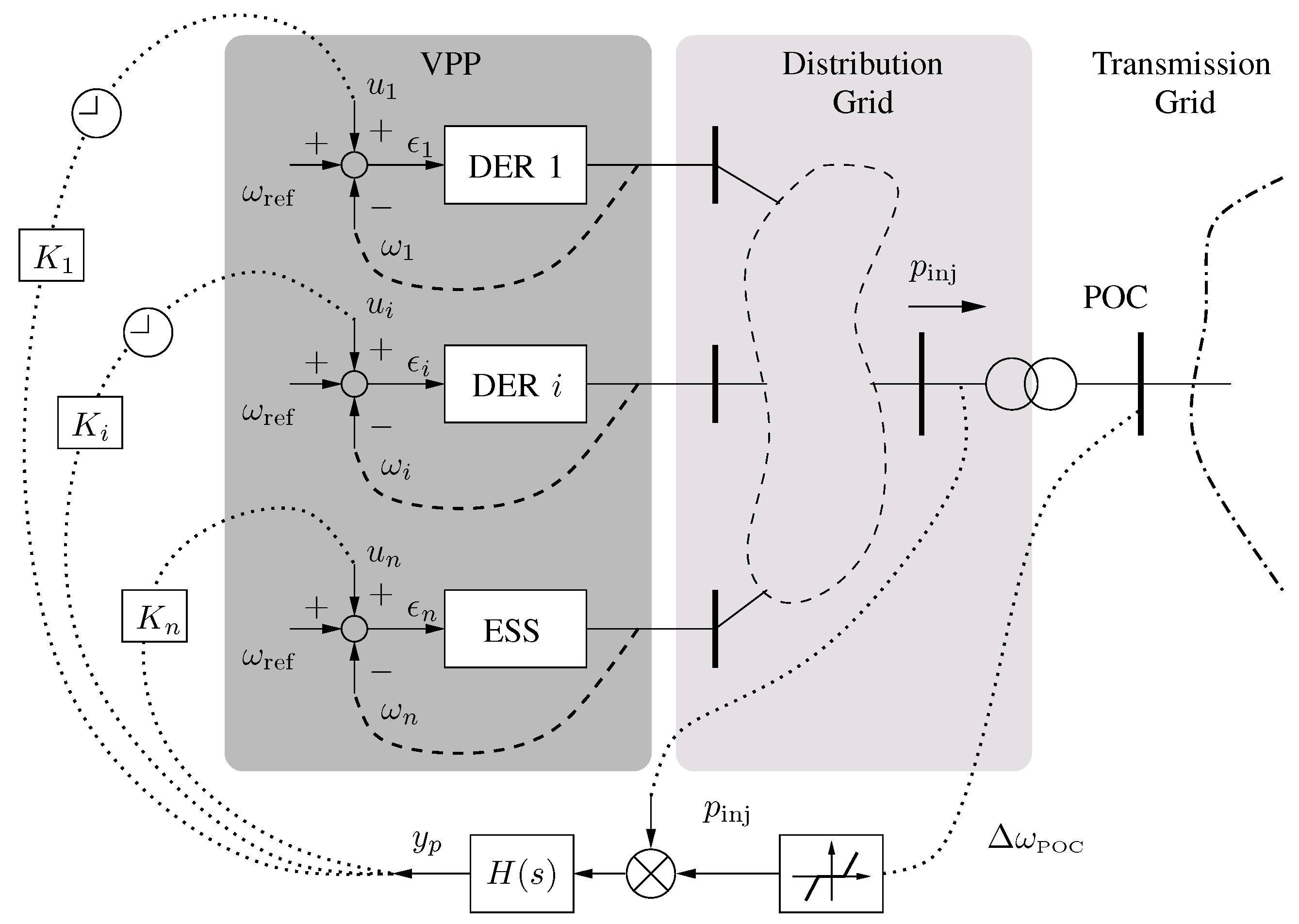
2.1. Proposed Coordinated Control

Figure 1 shows the proposed coordinated control of the resources that compose a VPP. This control is similar to a conventional secondary frequency control. However, it is aimed at improving the fast frequency response of the VPP and, thus, it operates in the same time scale as the primary frequency control.
It is assumed that in normal operating conditions and in a given period, the VPP power set-point is defined by the Transmission System Operator (TSO) based on the solution of an electricity market problem such as the unit commitment. Hence, before the occurrence of any contingency, p inj is the set-point of the VPP as scheduled by the TSO.
The proposed approach consists of measuring the total active power injected ( p inj ) into the transmission grid by the VPP as well as the frequency variation ( Δ ω POC ) and then transmitting the following signal:
y p = H ( s ) Δ ω POC p inj
to the DERs and ESSs that compose the VPP. In (1), H ( s ) is the transfer function of the coordinated control. H ( s ) includes a proper gain that adjusts the magnitude of y p and makes it consistent and compatible with the primary frequency controllers of the resources of the VPP. Apart from the proportional controller considered in (1), other controllers such as Proportional-Integral (PI) and lead-lag can also be used. The case study in Section 4 compares and discusses the performance of different controllers.
The rationale of the proposed coordinated controller is as follows. In steady-state conditions, Δ ω POC = 0 and hence the primary controllers of the resources that form the VPP are decoupled. For practical implementation issues, a small dead-band is then included on the signal Δ ω POC , to avoid unnecessary communications of the signal y p when the frequency deviations are negligible. The dead-band is used only to make the coordinated control insensitive to noise.
After the occurrence of a major contingency in the transmission grid, e.g., a fault or the outage of a large load/generator, the frequency of the system varies. This event leads to Δ ω POC 0 and thus triggers the coordinated feedback control.
The effect of y p is, in turn, to “amplify” the sensitivity of the primary control with respect to the local frequency deviation by a coefficient that is proportional to the power generated by the VPP. In fact, assuming that Δ ω POC measured at the POC is the same as the local frequency deviation measured by the DERs, one has that the overall signal entering the primary frequency controllers is:
ϵ i = ( ω ref ω i ) + u i [ 1 + K i H ( s ) p inj ] Δ ω POC ,
where ω ref ω i is the local frequency error as measured by the ESS or DER controller; and u i = K i y p .
Figure 1 shows that timers are included in the signals sent to the DERs. These timers are triggered by a threshold value of u i and allows improving the coordination of the DERs and ESSs. This point is duly discussed and illustrated in the case study.

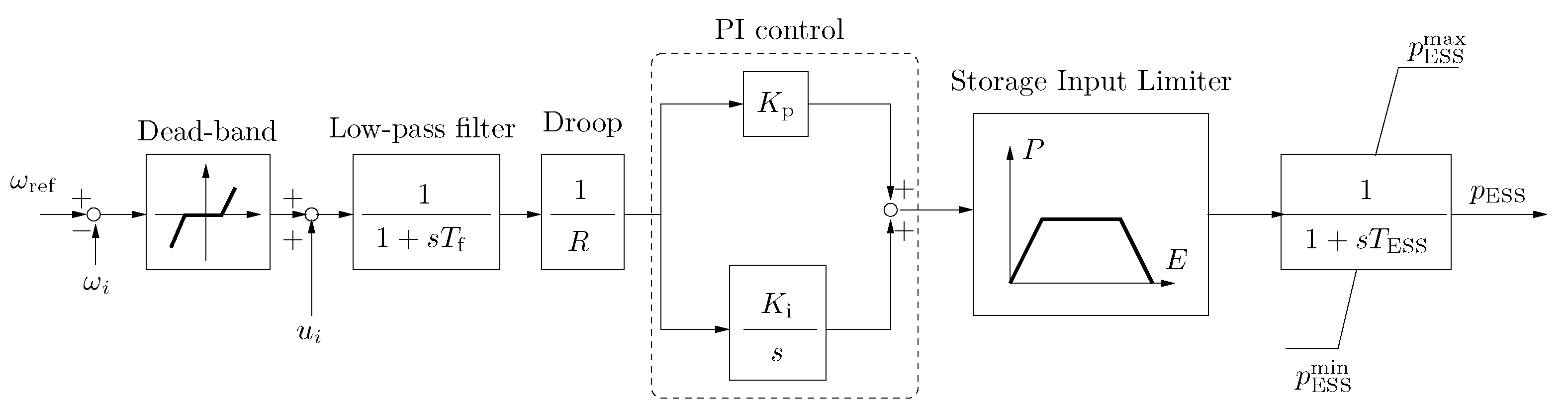
2.2. Frequency Control of Energy Storage Systems

ESSs can be used to improve the transient behavior of low-inertia systems. In this paper, we use the ESS control structure shown in Figure 2 and proposed in [28]. The controller includes a Storage Input Limiter (SIL) to smooth the transients that derive from the energy saturation/exhaustion of the ESS. The input signal is the deviation of the measured frequency ω i with respect to a reference frequency ω ref . The frequency error is processed by the devices through a Dead-band (DB), a Low pass filter (LPF), a frequency controller composed of a PI controller and droop controller, and a SIL as well as an anti-windup first-order lag filter. The coordinated signal u i is added between the DB and the LPF. The last block of Figure 2 represents the actual energy storage device and its output p ESS is the active power injected by the ESS into the grid.

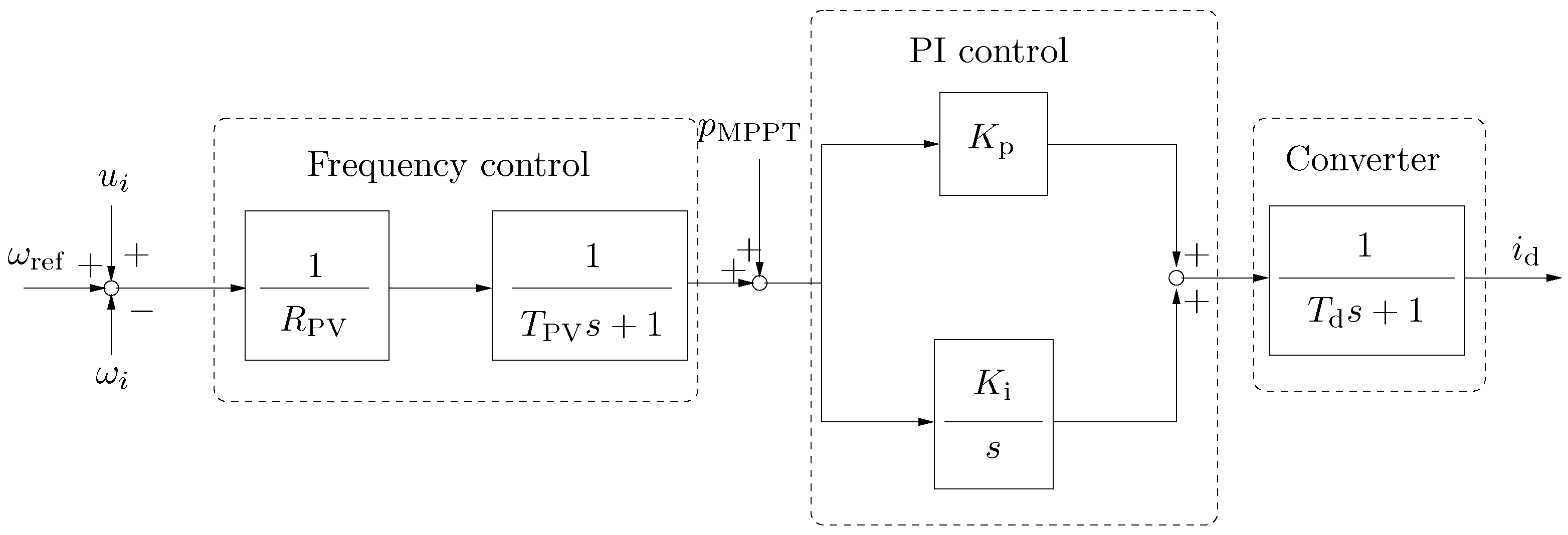
2.3. Frequency Control of Solar Photo-Voltaic Generation

The SPVG frequency control scheme used in this paper is shown in Figure 3 [29]. The scheme consists of a frequency control composed of droop gain and a LPF to eliminate ω ref ω i and u i . The output signal is added to the Maximum Power Point Tracking (MPPT) reference power and then processed by a PI controller, which imposes the d-axis current of the SPVG converter. The last block of Figure 3 represents the converter that connects the PV panel to the AC grid. Its output is the d -axis component of the current ( i d ) that injected by the PV panel into the grid.

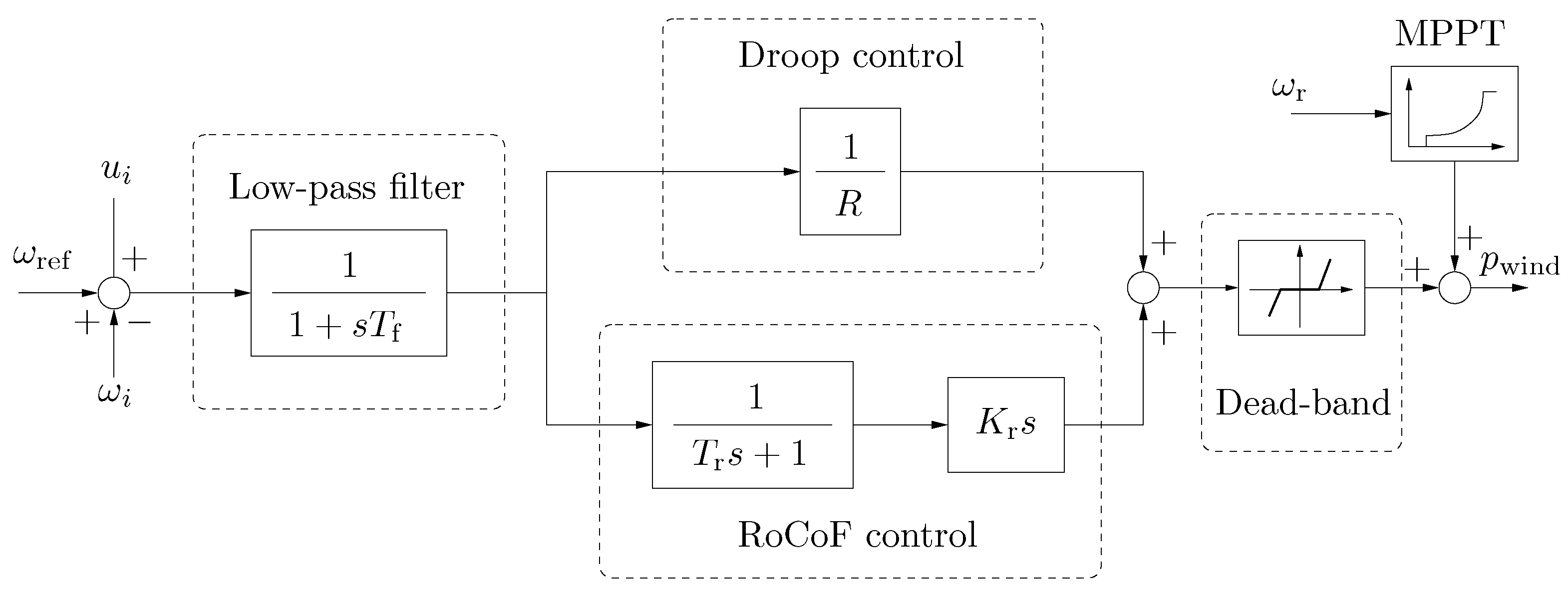
2.4. Frequency Control of Wind Power Plants

The frequency controller of wind turbines is shown in Figure 4 [30]. This controller is coupled with the MPPT output and includes a droop control and a Rate of Change of Frequency (RoCoF) control, where the LPF is used to filter out noises. The dead-band is used to enable the frequency control only if its output signal is above a given threshold. The output quantity p wind shown in Figure 4 represents the active power reference signal that is used in the converter of the wind turbine and that imposes the actual active power generation of the WG.

2.5. VPP Control Modes

In this subsection, we consider different coordinated control methods for ESS and DERs in VPP.
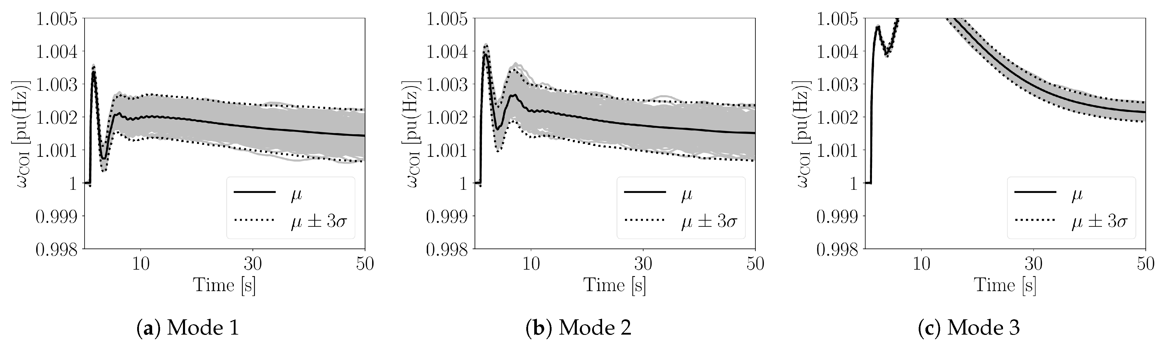
  • Mode 1: DERs and ESSs regulate the frequency but are fully independent ( y p = 0 ).
  • Mode 2: Only ESSs regulate the frequency. DERs do not include a frequency controller.
  • Mode 3: DERs do not include a frequency control. The ESS is regulated to keep constant the power injection p inj of the VPP into the POC. This is a typical VPP operation mode, where TSO schedules the VPP output every 15 min.
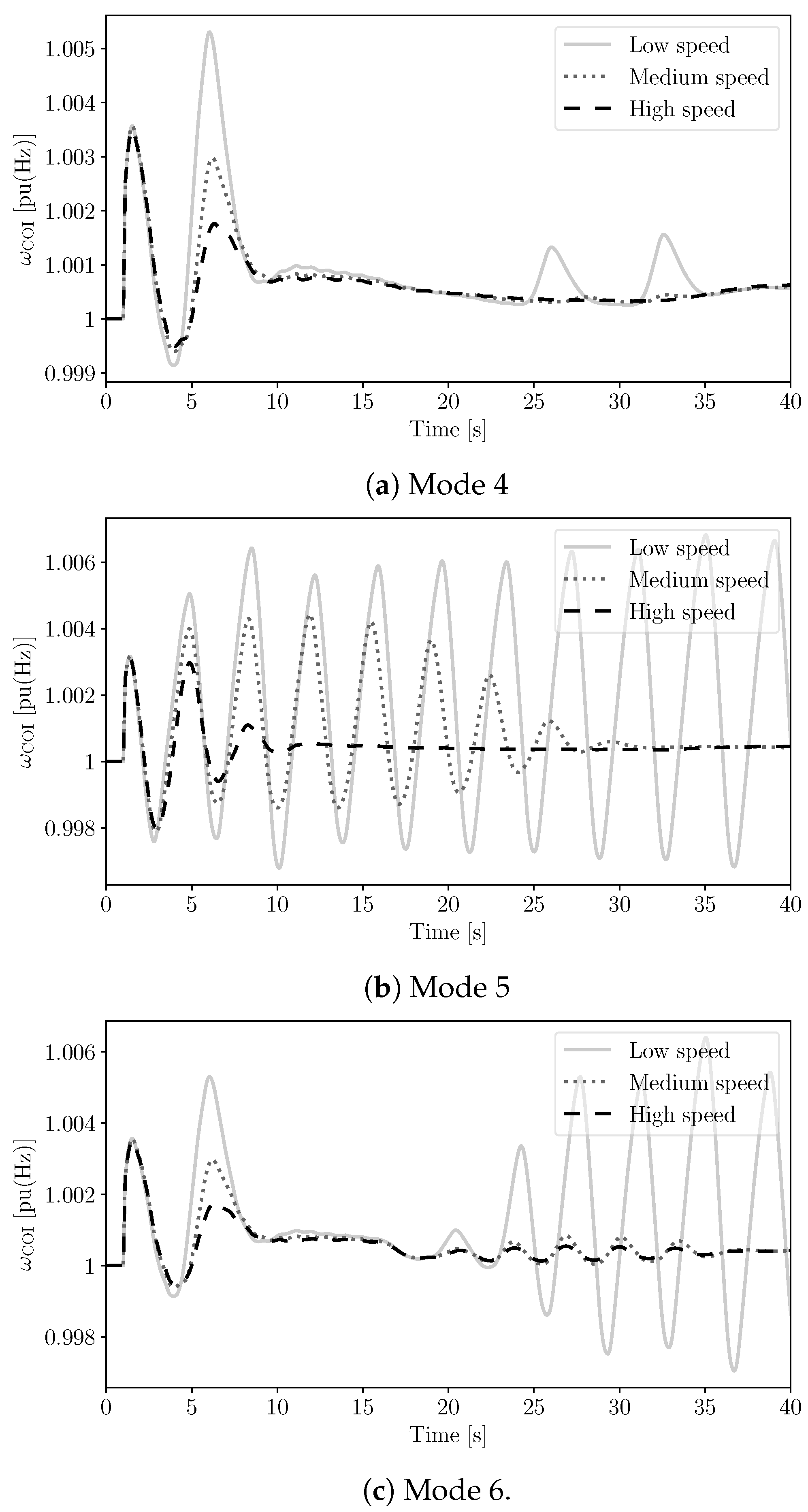
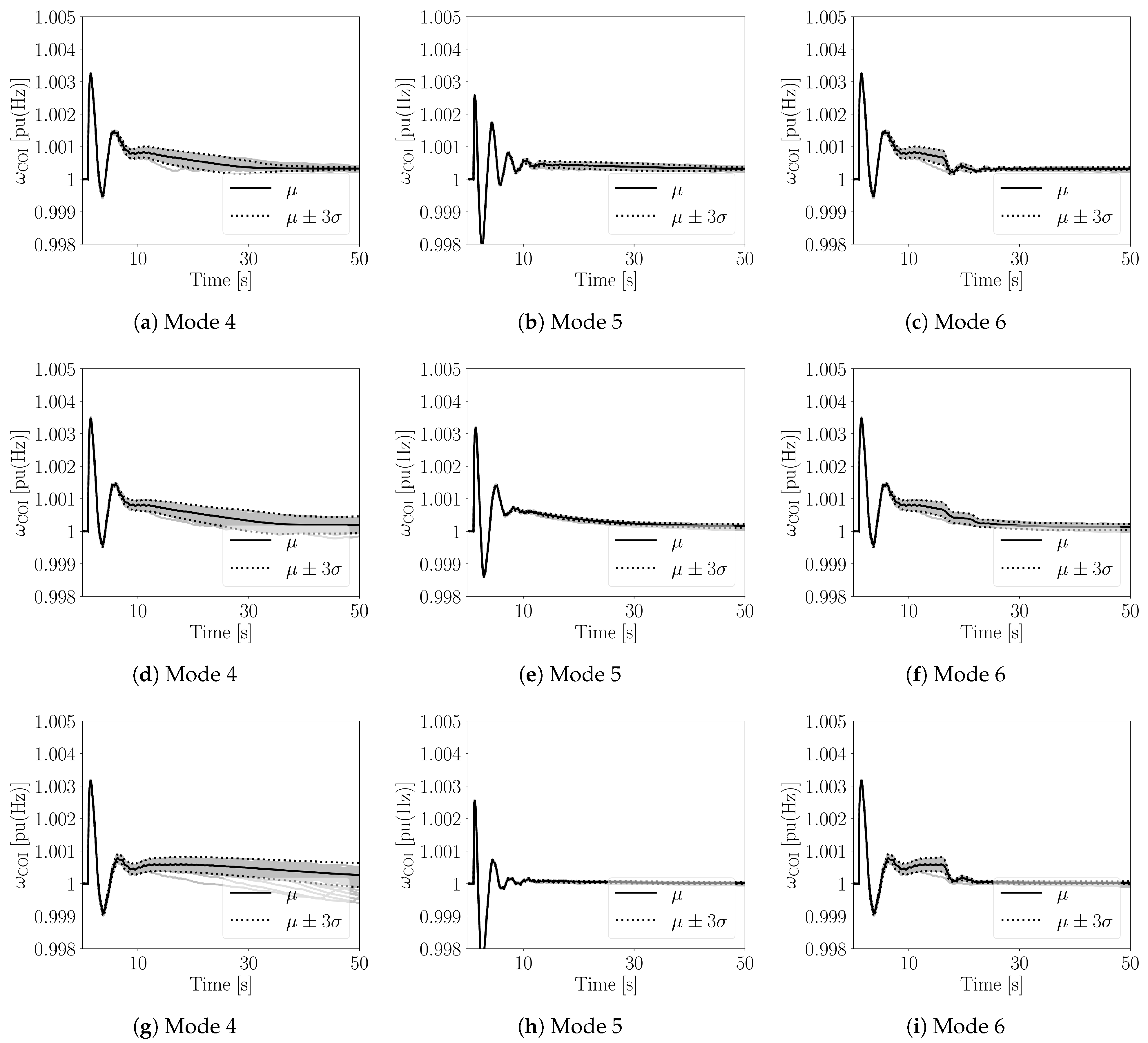
  • Mode 4: In [5], the weather-driven DERs such as WGs and SPVGs are considered to be non-dispatchable resources due to the stochastic nature of the wind and clouds. The ESS is the only device that regulates frequency. Therefore, in this mode, only the ESS is fed with the signal y p .
  • Mode 5: In [31], it is proposed that wind farms and VPPs can be used for emergency frequency control in smart super grids. Hence, in this mode, both ESS and DERs are coordinated with the signal y p .
  • Mode 6: As with Mode 5, both the ESS and DERs are coordinated in this mode. However, the feedback signal y p is used differently for ESSs and DERs. ESSs are always fed with y p and, thus, their primary frequency regulation acts immediately after the contingency. On the other hand, DERs are included in the coordinated control and receive the signal y p after a given time after the occurrence of the contingency, e.g., 15 s. The timer that activates the feedback signal for the DERs is triggered by the magnitude of the variation of the frequency Δ ω POC .

3. System Modeling

The power system model considered in this paper includes stochastic processes, which take into account wind and solar generation as well as load variations. Since the proposed coordinated control requires the transmission of remote signals, time delays are also considered to model the communication system. The resulting overall model of the system is the following set of Stochastic Delay Differential-Algebraic Equation (SDDAEs) [18,32]:
x ˙ = f ( x , y , y d , η , u ) , 0 = g ( x , y , y d , η , u ) , η ˙ = a ( x , y , η ) + b ( x , y , η ) ξ ,
where f and g are the differential and algebraic equations, respectively; x are the state variables, e.g., rotor angles/speeds of synchronous machines, the dynamic states of loads, etc.; y are the algebraic variables, e.g., bus frequency and bus voltage magnitudes/phases, and the active power output of generators; y d = y ( t τ ) are the delayed algebraic variables; η are the stochastic perturbations; u are the input variables, e.g., faults and line outages; a and b are the drift and the diffusion terms of the Stochastic Differential Equation (SDE) respectively and ξ represents the white noise, i.e., the formal time derivative of the Wiener processes. The stochastic models of voltage-dependent load, wind, and solar irradiance are based on [32,33,34], respectively. The interested reader can find a detailed description of these stochastic models in these references. The delay included in (3) models communication network issues, e.g., latency, packet dropout and jitter involved in the transmission of the measurements and control signals in the proposed coordinated control of the VPP. Following the requirements of the VPP communication system described in [35,36], in this paper, the communication delay in (3) is modeled as a Wide-Area Communication (WAC) delay, as follows [37,38]:
τ ( t ) = τ f + τ p ( t ) + θ ( t ) ,
where τ is the total communication delay, τ f is the fixed constant delay associated with sensors (e.g., Phase-Locked Loop (PLL) or Phasor Measurement Unit (PMU)) and data processing; τ p is the transmission delay; and θ is the random jitter.
The transmission delay is formulated as:
τ p = τ p o + S B ,
where τ p o is the propagation delay determined by the transmission medium (e.g., optical fiber, WIFI, or WLAN), S is the packet size of each data, and B is the transmission channel bandwidth. Finally, the random jitter θ in (4) includes the effect of noise, network topology, routing protocol, and background traffic.
In the following we assume that the frequency signal Δ ω POC and power injection p inj transmitted from meters to the control center are delayed, as follows:
Δ ω POC , d = Δ ω POC ( t τ ( t ) ) , p inj , d = p inj ( t τ ( t ) ) ,
where Δ ω POC , d and p inj , d are the delayed measurements, hence y d = [ Δ ω POC , d , p inj , d ] . Please note that all communication systems delays are included in Δ ω POC , d and p inj , d , thus there is no need to model the delay in the signal y p that is sent to DERs and ESSs.

3.1. Stochastic Wind

To emulate the wind speed as a stochastic process with Weibull distribution and exponential autocorrelation, a ( · ) and b ( · ) in (3) are solved [33]. The following drift and diffusion terms are obtained:
a ( x ( t ) ) = α · ( x ( t ) μ W ) b ( x ( t ) ) = b 1 ( x ( t ) ) · b 2 ( x ( t ) ) ,
with
b 1 ( x ( t ) ) = 2 · α p W ( x ( t ) ) b 2 ( x ( t ) ) = λ · Γ 1 + 1 k , x ( t ) λ k μ W · e x ( t ) / λ k ,
where α is the autocorrelation coefficient; μ W is the mean of the Weibull distribution; p W ( · ) is the Probability Density Function (PDF) of the Weibull distribution; Γ ( · , · ) is the Incomplete Gamma function; k and λ are the shape and scale parameters of the Weibull distribution, respectively.

3.2. Stochastic Load

The equations of the stochastic voltage-dependent load model are proposed in [32] as follows:
p L ( t ) = ( p L 0 + η p ( t ) ) ( v ( t ) / v 0 ) γ q L ( t ) = ( q L 0 + η q ( t ) ) ( v ( t ) / v 0 ) γ η ˙ p ( t ) = α p ( μ p η p ( t ) ) + b p ξ p η ˙ q ( t ) = α q ( μ q η q ( t ) ) + b q ξ q ,
where p L 0 and q L 0 are the active and reactive powers at t = 0 ; v ( t ) is the voltage magnitude of the bus where the load is connected; v 0 the voltage magnitude at t = 0 ; and γ is the power exponent where γ = 0 means constant power loads; the α terms are the mean-reversion speed at which the stochastic variables η are dragged towards the mean values μ ; and the b terms represent the volatility of the processes.

3.3. Stochastic Solar Irradiance

The following clear-sky index is used to model the solar irradiance as proposed in [34]:
k ( t ) = X ( t ) + κ ( t ) G ( t ) ,
where k ( t ) is the clear-sky index; X ( t ) is defined by the Ornstein–Uhlenbeck SDE in (3); κ ( t ) = { 0 , 1 } is the duration of a clouding event; and G ( t ) represents the Poisson jump process of the solar irradiance variability.

4. Case Study

This case study considers a modified version of the well-known WSCC 9-bus, 3-machine test system [39], where the load at bus 6 is replaced with a 8-bus, 38 kV distribution system that includes a VPP [40]. The topology of the overall system is shown in Figure 5. Specific setups are as follows.
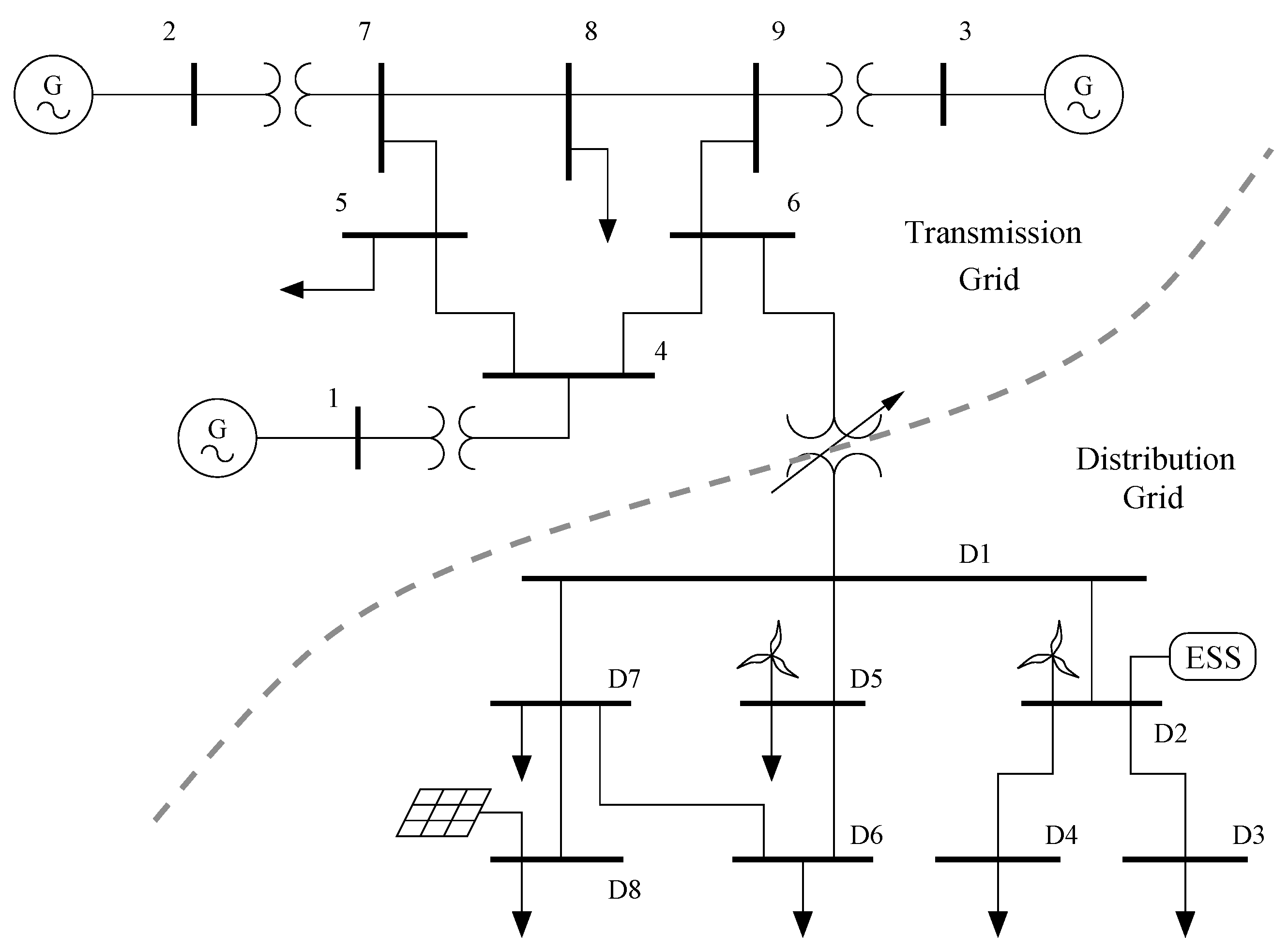
  • The VPP is connected through an Under-Load Tap Changer (ULTC) type step down transformer with TG.
  • One SPVG, two WGs, and one ESS are connected at buses D8, D5, D2, and D2, respectively. Each DER uses the bus frequency signal by an Synchronous Reference Frame Phase-Locked Loop (SRF-PLL) installed at Bus D1 for frequency control. The initial active power generation of the WG and the SPVG are 15 MW each, whereas the power rate of the ESS is 10 MW.
  • The total active and reactive power consumption of loads in the VPP are 57.8 MW and 11.7 MVar, respectively.
  • Since the focus of the case study is to observe the power system short-term transient behavior (a few tens of seconds), the impact of the State of Charge (SoC) of ESS is neglected.
In this case, the power injected by the VPP into the grid, namely p inj , is the power flow from Bus D1 to Bus 6. The stochastic processes of the wind speeds, load consumption and solar irradiance described in the previous section are included in all scenarios of the case study. Simulations are carried out using the co-simulation software tool described in [41] that combines the Python-based power system simulator Dome [42] and the communication network simulator ns-3 [43].

4.1. Monte Carlo Analysis

This section discusses the robustness of the proposed control approach concerning the perturbations such as a three-phase fault at bus 7 occurring at t = 1 s and cleared after 100 ms. The stochastic perturbations are the power variations of wind and solar power plants with respect to the forecast of wind speed/solar irradiance, and 15% of the loads in the whole system. For each scenario, 500 Monte Carlo time domain simulations are solved. Figure 6 shows the frequency trajectories for the system that VPP without frequency control on DERs and without ESS. The trajectories of the frequencies for Modes 1 to 3 are shown in Figure 7, whereas the trajectories of the frequency for Modes 4 to 6 with three different transfer functions H ( s ) are shown in Figure 8. The considered transfer functions are the most commonly used controllers such as proportional gain, PI controller and lead-lag controller. For all controllers, the parameters the lead to the best dynamic performance are selected through a trial-and-error approach. For simplicity, and since the size of all DERs and the ESS is similar, K i = 1 , i = 1 , , n . Finally, Table 1 shows the mean frequency, μ COI , as well as the standard deviation of the frequency σ COI , calculated at t = 50 s, for the six control modes and the three transfer functions H ( s ) considered in this case study.
The comparison of Figure 6, Figure 7 and Figure 8 indicates that the VPP without DER frequency control and without ESSs leads to the largest frequency deviation in the system. Please note that the results shown in Figure 6 can be also viewed as the worst-case scenario representing the complete outage of the communication network in the VPP. The comparison of the trajectories shown in Figure 7 and Figure 8 as well as of the results given in Table 1 indicates that the VPP control modes that include the proposed coordinated approach control (Modes 4–6) have an overall better performance than the strategies with no coordination (Modes 1–3).
It is interesting to note that for Mode 4 (see Figure 8a,d,g,) , the standard deviation slightly increases for 10 < t < 30 s because the ESS is running at its maximum output that loses its capability to regulate the frequency. Coordinating the DERs, i.e., Mode 5, to provide extra frequency support can help to solve this problem as shown in Figure 8b,e,h. However, this leads to a larger frequency deviation during the initial transients ( 0 < t < 10 s). Finally, Mode 6, where a timer is used to delay the action of DERs, shows the best dynamic performance (see Figure 8c,f,i).
The results shown in Figure 8 are obtained with the best set of parameters for each controller, namely proportional gain, lead-lag controller, and PI controller. For the PI controller, a small dead-band on the frequency deviation Δ ω POC . Although all controllers perform well, they have different performance depending on the mode. The PI controller performs best if both ESS and DERs regulate the frequency. However, if only the ESS is used to regulate the frequency, the PI controller leads more often the ESS to its maximum power output, thus making the control less efficient as with the proportional controller and lead-lag. All controllers perform well for Mode 6, i.e., when a timer shifts the action of the DERs. The timer in fact exploits the ability of the ESS to regulate the frequency in the first seconds but avoids ESS saturations in the longer term.

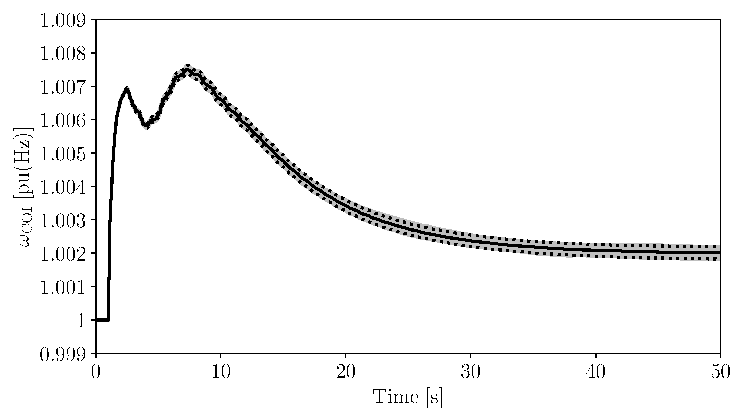
4.2. Impact of Communication Delays

As mentioned in Section 3, there exists a delay when the frequency signal Δ ω POC and active power p inj transmitted through the communication network. In this section, the communication delay with respect to three levels of communication networks, namely high-speed, middle-speed, and low-speed communication networks are considered. All the remote signals are considered to be 100 bytes PMU data with a reporting rate of 25 frames per second. UDP/IP protocol is adopted to avoid the data re-transmission for reducing the communication delay, where the physical link layer of the communication network is a Point-to-Point link. The background traffic consists of both 500 bytes Remote Terminal Unit (RTU) data with a reporting rate of 2 frames per second, and 1024 bytes video streams, 200 frames per second, respectively. Table 2 shows the parameters of the communication network for each scenario.
Most real-world communication networks used in power system applications are somewhere in between the high-speed and medium-speed communication networks depicted in Table 2. However, low-bandwidth communication networks are cheaper and, thus, the low-speed communication network is also considered here. Clearly, the lower the speed (bandwidth) of the communication network, the higher the delays of the control signals.
Figure 9 shows the impact on the frequency of the COI of communication delays as obtained with the three communication networks of Table 2. The system undergoes the same three-phase fault considered in Section 4.1. Only Modes 4, 5 and 6 are compared as these are the modes that require a communication network. Simulation results, which were obtained using the proportional controller, indicate that the proposed coordinated control approach, especially Modes 5 and 6 are particularly impacted by communication delays.
When the communication network has a low bandwidth with a large time-varying delay of around 200 ms, the approach that only coordinates the ESS gives rise to an oscillation on the system frequency (see the interval between 25 and 35 s in Figure 9a). Mode 6 sharply increases this oscillation. Then in the medium-speed communication network with a medium time-varying delay of around 100 ms, the performances for Modes 4 and 6 are acceptable; however, for Mode 5, the frequency oscillation is still significant. Finally, the delays of the high-speed communication network are around 55 ms. This delay has only a slight impact on the overall frequency behavior. Based on the simulation results, it appears, thus, that communication delays should be kept below 100 ms when the proposed coordinated control approach is adopted.
It is important to note that due to the nonlinearity of the model of the power systems, it is not possible to draw general conclusions on the impact of delays. However, based on our knowledge and experience with several systems and scenarios, communication delays in control loops can be expected to worsen the dynamic response of the system and reduce its stability margin (see for example [18,38]).

5. Conclusions

This paper proposes a coordinated control method of VPP to improve power system short-term transient frequency response. The proposed strategy is based on a coordinated control of DERs and ESSs in the VPP. A variety of control modes are compared and validated through Monte Carlo simulations. The impact of communication delays, stochastic processes as well as of the capacity of ESS on the overall transient behavior are also outlined. Based on the simulation results, the following conclusions can be drawn.
1.
The proposed coordinated control approach for ESS and DERs in VPP can significantly improve power system frequency stability. The proposed control approach performs better than either conventional VPPs that do not regulate the frequency, i.e., use a constant power set-point, and VPPs that regulate the frequency through the independent controllers of ESSs and DERs.
2.
Communication delays have a significant impact on the proposed coordinated control approach. This had to be expected, as the proposed strategy works as a sort of fast secondary frequency control. To reduce the negative impact of communication networks without increasing the bandwidth, a two-phase coordinated control is proposed. In this operating mode, the ESS acts first whereas DERs are included in the coordinated control in a second phase. This reduces the impact of the limited capacity of the ESS and, in turn, improves the transient stability.
Future work will focus on further improving the short-term frequency control of DERs and ESS included in VPPs. For example, ad hoc feedback transfer functions for each DER and ESS rather than a single common H ( s ) will be considered. Secondary frequency control of VPPs will be also considered, thus allowing taking into account the state of charge of ESSs and short-term weather forecast. The impact of cybersecurity in a communication network includes bad data will also be also considered.

Author Contributions

All authors equally contributed to this work. All authors have read and agreed to the published version of the manuscript.

Funding

This work was supported by Science Foundation Ireland, by funding W.Z. and F.M. under project ESIPP, Grant No. SFI/15/SPP/E3125; and M.A.A.M., M.L. and F.M. under project AMPSAS, Grant No. SFI/15/IA/3074; and J.C. and F.M. under project EdgeFLEX, Grant No. 883710.

Institutional Review Board Statement

Not applicable.

Informed Consent Statement

Not applicable.

Conflicts of Interest

The authors declare no conflict of interest.

References

  1. Palizban, O.; Kauhaniemi, K.; Guerrero, J.M. Microgrids in active network management—Part I: Hierarchical control, energy storage, virtual power plants, and market participation. Renew. Sustain. Energy Rev. 2014, 36, 428–439. [Google Scholar] [CrossRef] [Green Version]
  2. Pudjianto, D.; Ramsay, C.; Strbac, G. Virtual power plant and system integration of distributed energy resources. IET Renew. Power Gener. 2007, 1, 10–16. [Google Scholar] [CrossRef]
  3. Ruiz, N.; Cobelo, I.; Oyarzabal, J. A direct load control model for virtual power plant management. IEEE Trans. Power Syst. 2009, 24, 959–966. [Google Scholar] [CrossRef]
  4. Liu, Y.; Xin, H.; Wang, Z.; Gan, D. Control of virtual power plant in microgrids: A coordinated approach based on photovoltaic systems and controllable loads. IET Gener. Transm. Distrib. 2015, 9, 921–928. [Google Scholar] [CrossRef] [Green Version]
  5. Morales, J.M.; Conejo, A.J.; Madsen, H.; Pinson, P.; Zugno, M. Virtual power plants. In Integrating Renewables in Electricity Markets; Springer: Berlin, Germany, 2014. [Google Scholar]
  6. Olivares, D.E.; Mehrizi-Sani, A.; Etemadi, A.H.; Cañizares, C.A.; Iravani, R.; Kazerani, M.; Hajimiragha, A.H.; Gomis-Bellmunt, O.; Saeedifard, M.; Palma-Behnke, R.; et al. Trends in microgrid control. IEEE Trans. Smart Grid 2014, 5, 1905–1919. [Google Scholar] [CrossRef]
  7. Han, Y.; Li, H.; Shen, P.; Coelho, E.A.A.; Guerrero, J.M. Review of active and reactive power sharing strategies in hierarchical controlled microgrids. IEEE Trans. Power Electron. 2016, 32, 2427–2451. [Google Scholar] [CrossRef] [Green Version]
  8. D’Arco, S.; Suul, J.A. Equivalence of virtual synchronous machines and frequency-droops for converter-based microgrids. IEEE Trans. Smart Grid 2013, 5, 394–395. [Google Scholar] [CrossRef]
  9. Ortega, Á.; Milano, F. Frequency control of distributed energy resources in distribution networks. IFAC-PapersOnLine 2018, 51, 37–42. [Google Scholar] [CrossRef]
  10. Zhong, W.; Murad, M.A.A.; Liu, M.; Milano, F. Impact of Virtual Power Plants on Power System Short-Term Transient Response. Electr. Power Syst. Res. 2020, 189, 106609. [Google Scholar] [CrossRef]
  11. Liu, M.; Chen, J.; Milano, F. On-line Inertia Estimation for Synchronous and Non-Synchronous Devices. IEEE Trans. Power Syst. 2020. [CrossRef]
  12. Vovos, P.N.; Kiprakis, A.E.; Wallace, A.R.; Harrison, G.P. Centralized and distributed voltage control: Impact on distributed generation penetration. IEEE Trans. Power Syst. 2007, 22, 476–483. [Google Scholar] [CrossRef] [Green Version]
  13. Savaghebi, M.; Jalilian, A.; Vasquez, J.C.; Guerrero, J.M. Secondary control scheme for voltage unbalance compensation in an islanded droop-controlled microgrid. IEEE Trans. Smart Grid 2012, 3, 797–807. [Google Scholar] [CrossRef] [Green Version]
  14. Meng, L.; Tang, F.; Savaghebi, M.; Vasquez, J.C.; Guerrero, J.M. Tertiary control of voltage unbalance compensation for optimal power quality in islanded microgrids. IEEE Trans. Energy Convers. 2014, 29, 802–815. [Google Scholar] [CrossRef] [Green Version]
  15. Acharya, S.; El-Moursi, M.S.; Al-Hinai, A.; Al-Sumaiti, A.S.; Zeineldin, H.H. A control strategy for voltage unbalance mitigation in an islanded microgrid considering demand side management capability. IEEE Trans. Smart Grid 2018, 10, 2558–2568. [Google Scholar] [CrossRef]
  16. Kim, J.; Lin, X.; Shroff, N.B. Optimal anycast technique for delay-sensitive energy-constrained asynchronous sensor networks. IEEE/ACM Trans. Netw. 2010, 19, 484–497. [Google Scholar] [CrossRef] [Green Version]
  17. Gelman, J.R.; Stadler, J.S. Method and Apparatus for Improving Efficiency of TCP/IP Protocol over High Delay-Bandwidth Network. US Patent 6,415,329, 2 July 2002. [Google Scholar]
  18. Milano, F.; Anghel, M. Impact of time delays on power system stability. IEEE Trans. Circ. Syst. I Regul. Pap. 2011, 59, 889–900. [Google Scholar] [CrossRef]
  19. Kekatos, V.; Wang, G.; Conejo, A.J.; Giannakis, G.B. Stochastic reactive power management in microgrids with renewables. IEEE Trans. Power Syst. 2014, 30, 3386–3395. [Google Scholar] [CrossRef] [Green Version]
  20. Yang, H.; Yi, D.; Zhao, J.; Dong, Z. Distributed optimal dispatch of virtual power plant via limited communication. IEEE Trans. Power Syst. 2013, 28, 3511–3512. [Google Scholar] [CrossRef]
  21. Schiffer, J.; Seel, T.; Raisch, J.; Sezi, T. Voltage stability and reactive power sharing in inverter-based microgrids with consensus-based distributed voltage control. IEEE Trans. Control Syst. Technol. 2015, 24, 96–109. [Google Scholar] [CrossRef] [Green Version]
  22. Simpson-Porco, J.W.; Shafiee, Q.; Dörfler, F.; Vasquez, J.C.; Guerrero, J.M.; Bullo, F. Secondary frequency and voltage control of islanded microgrids via distributed averaging. IEEE Trans. Ind. Electron. 2015, 62, 7025–7038. [Google Scholar] [CrossRef]
  23. Li, Q.; Chen, F.; Chen, M.; Guerrero, J.M.; Abbott, D. Agent-based decentralized control method for islanded microgrids. IEEE Trans. Smart Grid 2015, 7, 637–649. [Google Scholar] [CrossRef] [Green Version]
  24. Ahumada, C.; Cárdenas, R.; Saez, D.; Guerrero, J.M. Secondary control strategies for frequency restoration in islanded microgrids with consideration of communication delays. IEEE Trans. Smart Grid 2015, 7, 1430–1441. [Google Scholar] [CrossRef] [Green Version]
  25. Hosseinzadeh, M.; Sinopoli, B.; Garone, E. Feasibility and detection of replay attack in networked constrained cyber-physical systems. In Proceedings of the 57th Annual Allerton Conference on Communication, Control, and Computing, Monticello, IL, USA, 24–27 September 2019; pp. 712–717. [Google Scholar]
  26. Liu, Y.; Ning, P.; Reiter, M.K. False data injection attacks against state estimation in electric power grids. ACM Trans. Inf. Syst. Secur. 2011, 14, 1–33. [Google Scholar] [CrossRef]
  27. Chen, W.; Ding, D.; Dong, H.; Wei, G. Distributed resilient filtering for power systems subject to denial-of-service attacks. IEEE Trans. Syst. Man Cybern. Syst. 2019, 49, 1688–1697. [Google Scholar] [CrossRef]
  28. Ortega, Á.; Milano, F. Generalized model of VSC-based energy storage systems for transient stability analysis. IEEE Trans. Power Syst. 2015, 31, 3369–3380. [Google Scholar] [CrossRef] [Green Version]
  29. Tamimi, B.; Cañizares, C.; Bhattacharya, K. Modeling and performance analysis of large solar photo-voltaic generation on voltage stability and inter-area oscillations. In Proceedings of the IEEE PES General Meeting, Detroit, MI, USA, 24–28 July 2011; pp. 1–5. [Google Scholar]
  30. Morren, J.; De Haan, S.W.; Kling, W.L.; Ferreira, J.A. Wind turbines emulating inertia and supporting primary frequency control. IEEE Trans. Power Syst. 2006, 21, 433–434. [Google Scholar] [CrossRef]
  31. Arestova, A.; Sidorkin, Y. The use of wind farms and virtual power plants for emergency control in the future smart super grids. In Proceedings of the 2011 6th International Forum on Strategic Technology, Harbin, China, 22–24 August 2011; pp. 437–442. [Google Scholar]
  32. Milano, F.; Zárate-Miñano, R. A systematic method to model power systems as stochastic differential algebraic equations. IEEE Trans. Power Syst. 2013, 28, 4537–4544. [Google Scholar] [CrossRef]
  33. Zárate-Miñano, R.; Mele, F.M.; Milano, F. SDE-based wind speed models with Weibull distribution and exponential autocorrelation. In Proceedings of the IEEE PES General Meeting, Boston, MA, USA, 17–21 July 2016; pp. 1–5. [Google Scholar]
  34. Jónsdóttir, G.M.; Milano, F. Modeling Solar Irradiance for Short-term Dynamic Analysis of Power Systems. In Proceedings of the IEEE PES General Meeting, Atlanta, GA, USA, 4–8 August 2019; pp. 1–5. [Google Scholar]
  35. Pasetti, M.; Rinaldi, S.; Manerba, D. A virtual power plant architecture for the demand-side management of smart prosumers. Appl. Sci. 2018, 8, 432. [Google Scholar] [CrossRef] [Green Version]
  36. Pahwa, A.; DeLoach, S.A.; Natarajan, B.; Das, S.; Malekpour, A.R.; Alam, S.S.; Case, D.M. Goal-based holonic multiagent system for operation of power distribution systems. IEEE Trans. Smart Grid 2015, 6, 2510–2518. [Google Scholar] [CrossRef]
  37. Naduvathuparambil, B.; Valenti, M.C.; Feliachi, A. Communication delays in wide area measurement systems. In Proceedings of the Thirty-Fourth Southeastern Symposium on System Theory (Cat. No. 02EX540), Huntsville, AL, USA, 19 March 2002; pp. 118–122. [Google Scholar]
  38. Liu, M.; Dassios, I.; Tzounas, G.; Milano, F. Stability analysis of power systems with inclusion of realistic-modeling WAMS delays. IEEE Trans. Power Syst. 2018, 34, 627–636. [Google Scholar] [CrossRef]
  39. Sauer, P.W.; Pai, M.A. Power System Dynamics and Stability; Prentice Hall: Upper Saddle River, NJ, USA, 1998. [Google Scholar]
  40. Murphy, C.; Keane, A. Local and remote estimations using fitted polynomials in distribution systems. IEEE Trans. Power Syst. 2016, 32, 3185–3194. [Google Scholar] [CrossRef] [Green Version]
  41. Zhong, W.; Liu, M.; Milano, F. A co-simulation framework for power systems and communication networks. In Proceedings of the In 2019 IEEE Milan PowerTech, Milano, Italy, 23–27 June 2019; pp. 1–6. [Google Scholar]
  42. Milano, F. A Python-based software tool for power system analysis. In Proceedings of the IEEE PES General Meeting, Vancouver, BC, Canada, 21–25 July 2013; pp. 1–5. [Google Scholar]
  43. Riley, G.F.; Henderson, T.R. The ns-3 network simulator. In Modeling and Tools for Network Simulation; Springer: Berlin, Germany, 2010. [Google Scholar]
Figure 1. Control diagram of the proposed coordinated control of VPPs.
Energies 14 01182 g001
Figure 2. Frequency controller of the ESS.
Energies 14 01182 g002
Figure 3. Frequency control of SPVGs.
Energies 14 01182 g003
Figure 4. Frequency control of WGs.
Energies 14 01182 g004
Figure 5. Modified WSCC 9-bus, 3-machine system with a VPP.
Energies 14 01182 g005
Figure 6. Trajectories of the frequency of the Center of Inertia (COI) without VPP frequency control and without ESS. The mean and the standard deviation of the frequency at t = 50 s are μ COI = 1.002 pu(Hz) and σ COI = 6.16 · 10 5 pu(Hz), respectively.
Energies 14 01182 g006
Figure 7. Trajectories of the frequency of the COI without the proposed coordinated control.
Energies 14 01182 g007
Figure 8. Trajectories of the frequency of the COI using: (ac) proportional gain; (df) lead-lag controller; and (gi) PI controller.
Energies 14 01182 g008
Figure 9. Frequency of the COI following a three-phase fault occurs in the TG, where the measurements Δ ω POC and p inj are transmitted through high/medium/low-speed communication networks, respectively.
Energies 14 01182 g009
Table 1. Mean frequency μ COI and standard deviation σ COI for different VPP control modes.
StatisticsMode 1Mode 2Mode 3
μ COI 1.001431 1.001511 1.002144
σ COI × 10 5 [pu(Hz)] 23.6 28.1 9.73
Control TypeStatisticsMode 4Mode 5Mode 6
Prop. Control μ COI [pu(Hz)] 1.000328 1.000323 1.000321
σ COI × 10 5 [pu(Hz)] 1.83 1.58 1.43
Lead-Lag μ COI [pu(Hz)] 1.000198 1.000155 1.000135
σ COI × 10 5 [pu(Hz)] 8.62 2.24 3.27
PI μ COI [pu(Hz)] 1.000267 1.000020 1.000023
σ COI × 10 5 [pu(Hz)] 12.4 1.37 1.60
Table 2. Parameters of the communication networks.
LevelsBandwidthPMU Data RateBackground Traffic
High Speed20 Mbps25 frames/sRTU, Video Stream
Medium Speed5 Mbps25 frames/sRTU, Video Stream
Low Speed1 Mbps25 frames/sN/A
Publisher’s Note: MDPI stays neutral with regard to jurisdictional claims in published maps and institutional affiliations.

