Day-Ahead MPC Energy Management System for an Island Wind/Storage Hybrid Power Plant

Abstract

This paper presents a multi-objective energy management system (EMS) to manage the power dispatch of a hybrid power plant (HPP), consisting of a grid-connected wind farm and a Li-ION battery storage system on the island of Guadeloupe’s electrical grid. Via a controller based on Model Predictive Control (MPC), the EMS solves the problem of optimization by considering the production forecast data and managing several operation rules, which ensures meet energy targets considered for a sustainable power dispatching plan. The proposed strategy is tested in a PowerFactory/MATLAB co-simulation environment.

1. Introduction

Heavy dependence on imported energy in islands is one of the most important issues for these territories. Currently, several problems are mostly related to imported fossil fuel energy dependence, freshwater availability and waste management [1]. This is why renewable energy resources have achieved high levels of penetration in island electricity production over recent years.

Renewable wind energy is one of the most used sources on islands. The variable nature and uncertainty of wind energy poses substantial challenges for the power systems operations, in particular for weak or isolated grids. For these reasons, the grid code related to wind power plants specifies the requirement for ensuring a controlled power output and the supply of ancillary services. It is necessary to reduce frequency fluctuations caused by the wind’s random behavior, which makes the scheduling more difficult while increasing the system’s operational costs [2,3].

Consequently, the installation of wind turbines (WT) is growing worldwide on a large-scale. Wind generation systems have intermittent power output due to the variability of wind speed. Thereby, the penalties related to the infringement of day-ahead bids become inevitable. These issues are amplified in the context of island grids, like Guadeloupe, and should be managed to enhance grid efficiency without affecting stability and energy quality [4,5].

A way of dealing with these problems consists of setting-up hybrid power plants (HPPs), which combine wind turbines with production or storage technologies. In order to manage the energy to mitigate the wind generated power fluctuations, HPPs can consider renewable sources coupled with conventional/renewable power production, e.g., wind-diesel hybrid systems [6,7], wind-thermal [8,9], wind-hydro [10,11], and wind-solar systems [12,13]. It is also possible to combine wind production with storage systems, like batteries, fuel cells, and/or hydrogen storage. In this way, it becomes possible to instantaneously inject power into the grid and back up the conventional generation systems [14,15,16]. Not only can hybrid power plants can accommodate several types of production and storage resources, but their integration into conventional power grids can also bring reliability and efficiency in order to supply the demand.

1.1. Literature Review

In order to achieve smooth HPP wind-storage operations, it is necessary to establish an optimal control operations. The energy storage units in a wind power-based hybrid facility can be configured in an aggregated way serving the whole wind farm, or it can be distributed so that there is a storage unit associated locally to each WT. These configurations can be managed through an energy management system. The objective of an energy management system (EMS) is to find the best compromise among the operation objectives which optimizes the performance of the generation facility. In order to find the most suitable management approach, several aspects must be considered. These include hybrid system design and operational requirements, as well as the control and optimization strategy.

Recent research has addressed EMS development for the power dispatch of grid-connected microgrids, considering HPPs that integrate wind turbines and energy storage systems in rural areas and island territories [2,17,18,19]. The objective here is to deal with high power availability periods by storing the surplus of power and releasing stored energy when there is a power shortage.

Relevant EMSs have been reported in the literature based on heuristic methods, which present low computational costs and allow quick results. However, this is achieved by optimum trading and accuracy for speed. For example, the control system makes possible the joint scheduling of energy and reserves of conventional units and hybrid power stations on the island of Crete (Greece) in a stochastic form [20]. In Reference [2], a multi-objective energy management system based on the fuzzy theory for the standalone microgrid on the island of Flinders is presented. Another example is presented in Reference [21], where a simulation tool for operating of a hybrid photovoltaic/wind plant coupled with hydro-pumping storage was built on the island of Corsica’s electrical network. However, these works do not consider forecasting algorithms for the production of renewable sources, which is a key way to optimize the HPP operations and make it more realistic.

Other reported works are based on deterministic approaches, which take advantage of the issue’s analytical properties, generating a sequence of points that converge with a globally optimal solution, like Reference [17], who have studied the technical and economic performance for a distributed electrical power system with micro hydro-power stations, WTs, and solar photovoltaic on an island located off the west coast of Scotland. The authors in Reference [18] have studied the effect of a large scale wind-battery plant in the autonomous power system of Samos Island, in the Aegean Archipelago, by implementing an optimal power flow analysis. However, these methods need to take into account different criteria for improving the EMS, like, for example, predicting wind production and the conditions for power dispatch operations.

Large scale HPPs brings great challenges with regards to transient voltage and frequency stability in the power systems. More recently, different energy management strategies based on supervisory control and data acquisition have been developed to ensure the stable operating of the HPPs with different configurations [22,23,24,25,26]. The aim of these EMSs ensures a suitable power dispatch while supplying ancillary services, like, for example, frequency and voltage regulation.

The power dispatch of the wind/storage HPP is a problem without a priory knowledge of future events in the environment. Indeed, the instant WT production and other measurements in the hybrid plant are input information received at every calculation to solve the optimization problem. This problem, therefore, requires reactive optimization. More recently, Model Predictive Control (MPC) has received greater attention from the energy management microgrids community. This control strategy has the ability to include both forecasts and newly updated information to determine the system’s future trajectories, while efficiently handling different kinds of constraints [27]. The main advantages of MPCs are the handling of constraints, as well as multi-variable and nonlinear models. Furthermore, it integrates the disturbances and future variations in the references to the optimization problem. Nonetheless, it is frequently combined with optimization methods, such as quadratic programming [28,29] or Pareto solutions [30].

Some of these MPC algorithms have been used to achieve economic objectives. This is the case of the authors in Reference [31], who propose a controller to operate at the pricing level in order to fulfill the user’s needs while minimizing the power purchased from the external grid. This proposal allows an optimal real-time power dispatch in a connected microgrid, whereas considering the lifespan battery. This kind of strategy is applicable to industrial or residential microgrids, as in Reference [32], where a dissipativity control based distributed economic predictive model is proposed to allow microgrid users to optimize their own benefits while ensuring the performance and stability of the residential microgrid.

In Reference [15], an MPC scheme is proposed for the interlinking converter in a hybrid AC/DC MicroGrid. The scheme allows the local power and voltage control and is connected to a second control stage, responsible for maintaining the power balance under varying generation and consumption conditions. In comparison with traditional linear cascades, the strategy requires less tuning work. Often, this method is used to include the Renewable Energy Sources (RES) production forecasts in the optimization problem, either in terms of the expected generation or in terms of the primary source, (wind speed, solar radiance, etc.) [14,27,33].

Despite all these research efforts, there are still a large number of challenges linked to criteria, such as combining production sources, different storage technologies, effective load management, profitability operations, etc. Depending on set functioning objectives, the EMS aims to improve the system’s performance by maximizing the use of resources and reducing the system’s operating costs, taking into account the global market, applications, and different technical aspects [34].

1.2. Contribution

In this paper, a Multi-objective EMS that guarantees compliance with the day-ahead power dispatching plan of a wind-storage HPP is developed. Such HPP consists of a grid-connected wind farm and Li-ION battery storage system. Via a controller based on MPC, several operation rules are managed, in order to solve the optimization problem taking into consideration production forecasting data.

The main contributions of this paper can be briefly summarized as follows:

• A comprehensive island microgrid multi-objective energy management problem is established, taking into account the day-ahead dispatch schedule commitment.
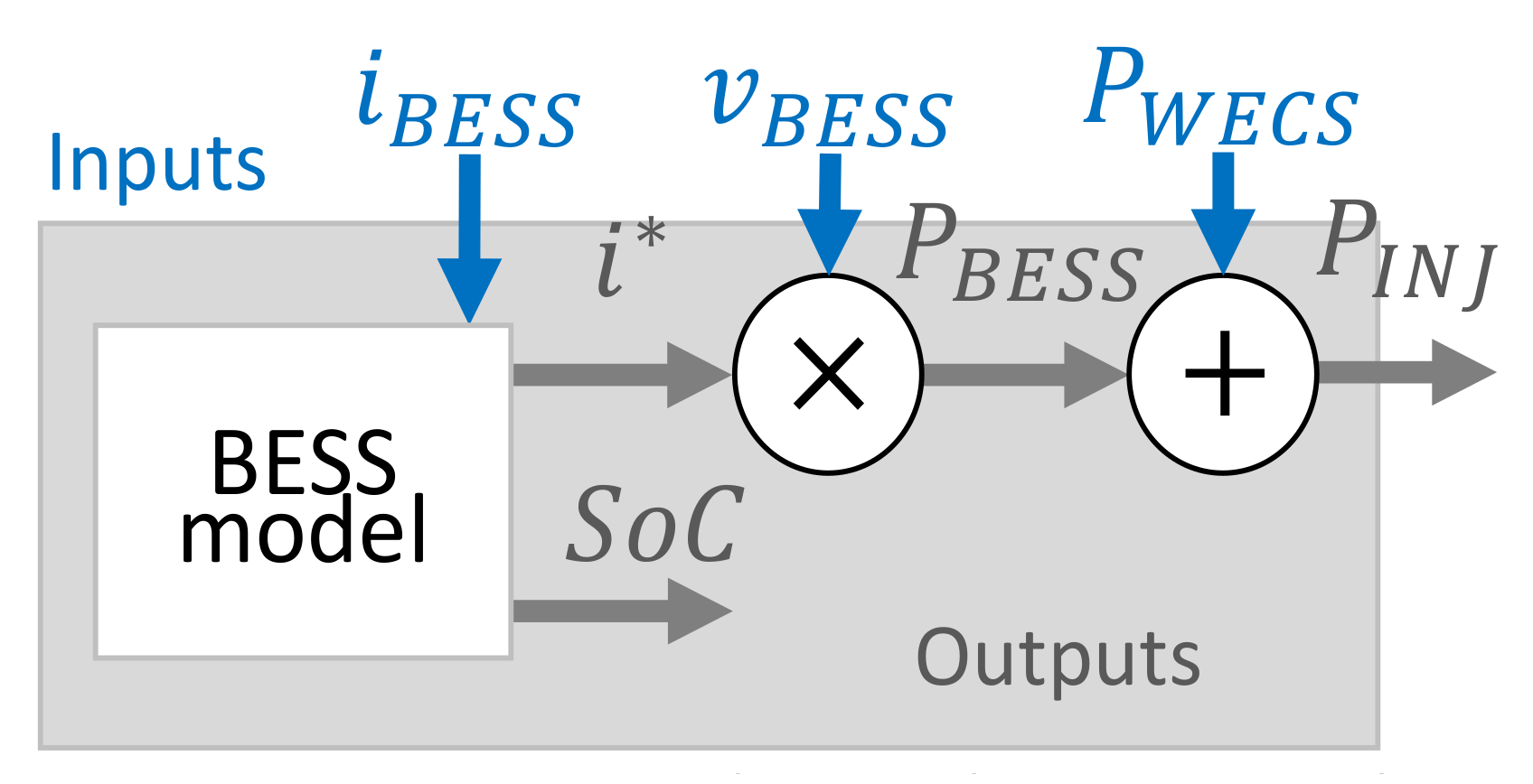
• The EMS proposed is able to manage the battery’s charge/discharge cycles and state-of-charge (SoC) efficiently. This is possible due to the development of a Battery Energy Storage System (BESS) model to find optimal solutions that bring the system’s predicted output close to a trajectory of defined future power injections.
• Through a model predictive control strategy, the EMS proposed allows the BESS to be optimized and, thereby, the power injection into the utility grid, while considering the battery’s lifespan.
• An evaluation of the proposed Multi-objective EMS by analyzing and comparing the simulation results from several study cases.

The EMS is tested in realistic scenarios via a PowerFactory/MATLAB co-simulation environment while taking into account the island grid’s real operations. Contrary to the paper by Reference [31], our strategy is not economic, but rather technical, which works by evaluating the technical conditions to supply the power commitment while avoiding economic penalties.

The organization of this paper is as follows. Section 2 presents a description of the Grid-connected wind-storage hybrid power plant. Section 3 presents the problem’s formulation. Section 4 introduces the models and validation of the different components which make up the wind-storage HPP. In Section 5, the multi-objective EMS based on the MPC, together with the optimization strategy, is developed, and, finally, in Section 6, the results are presented and discussed.

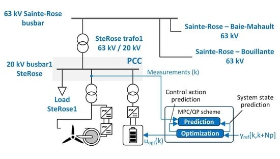
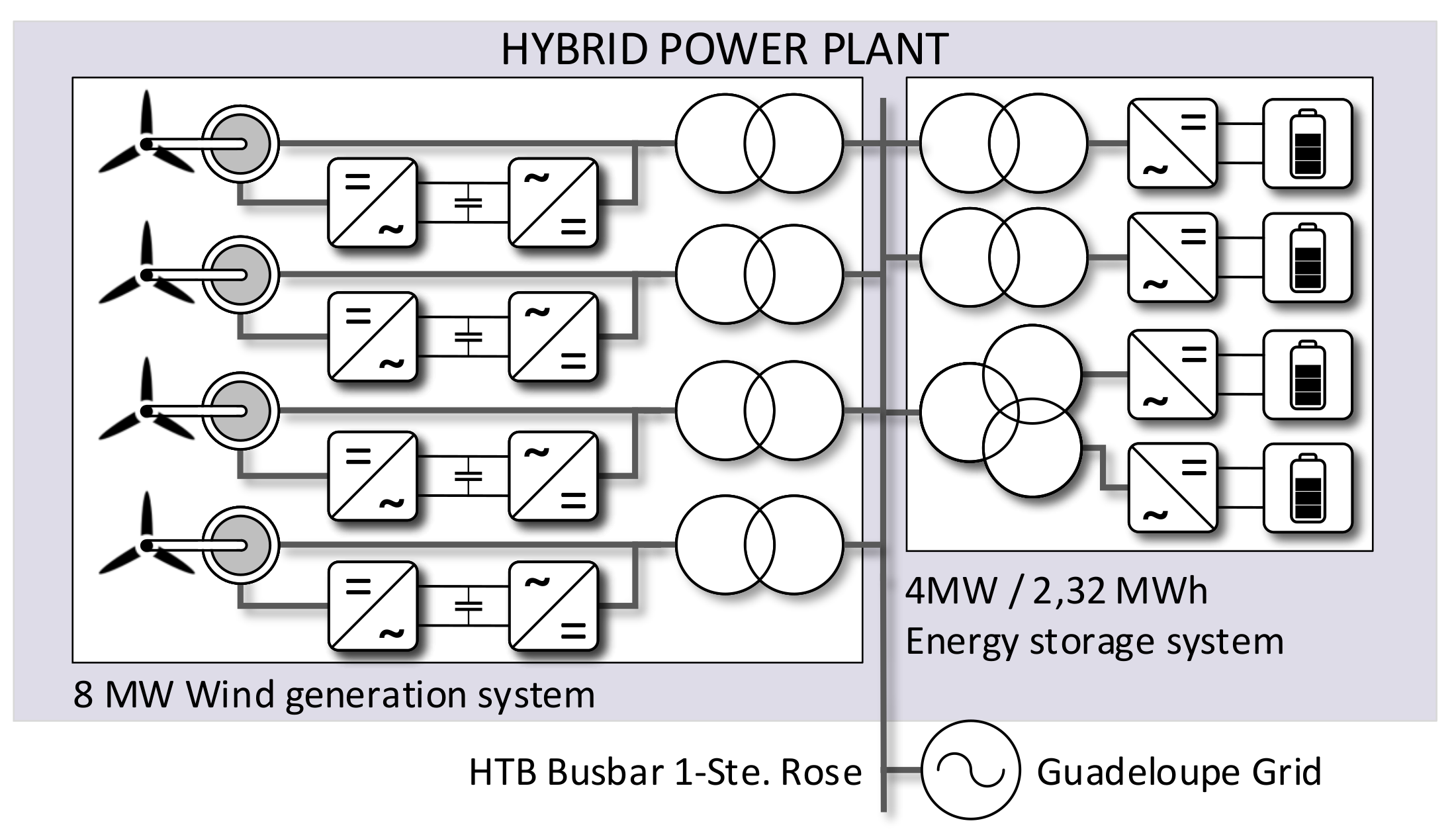
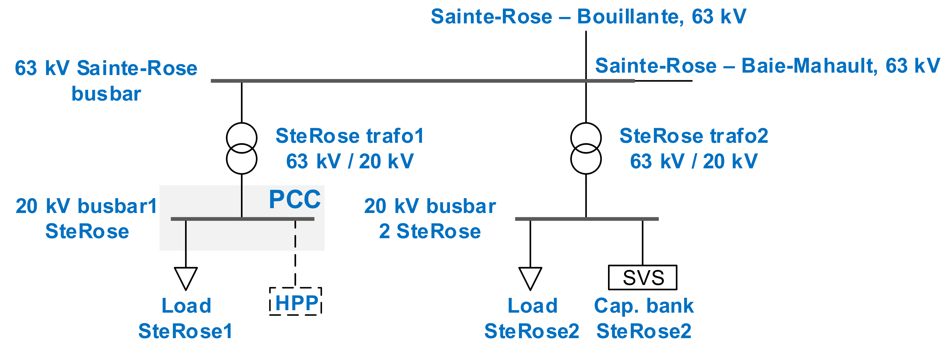
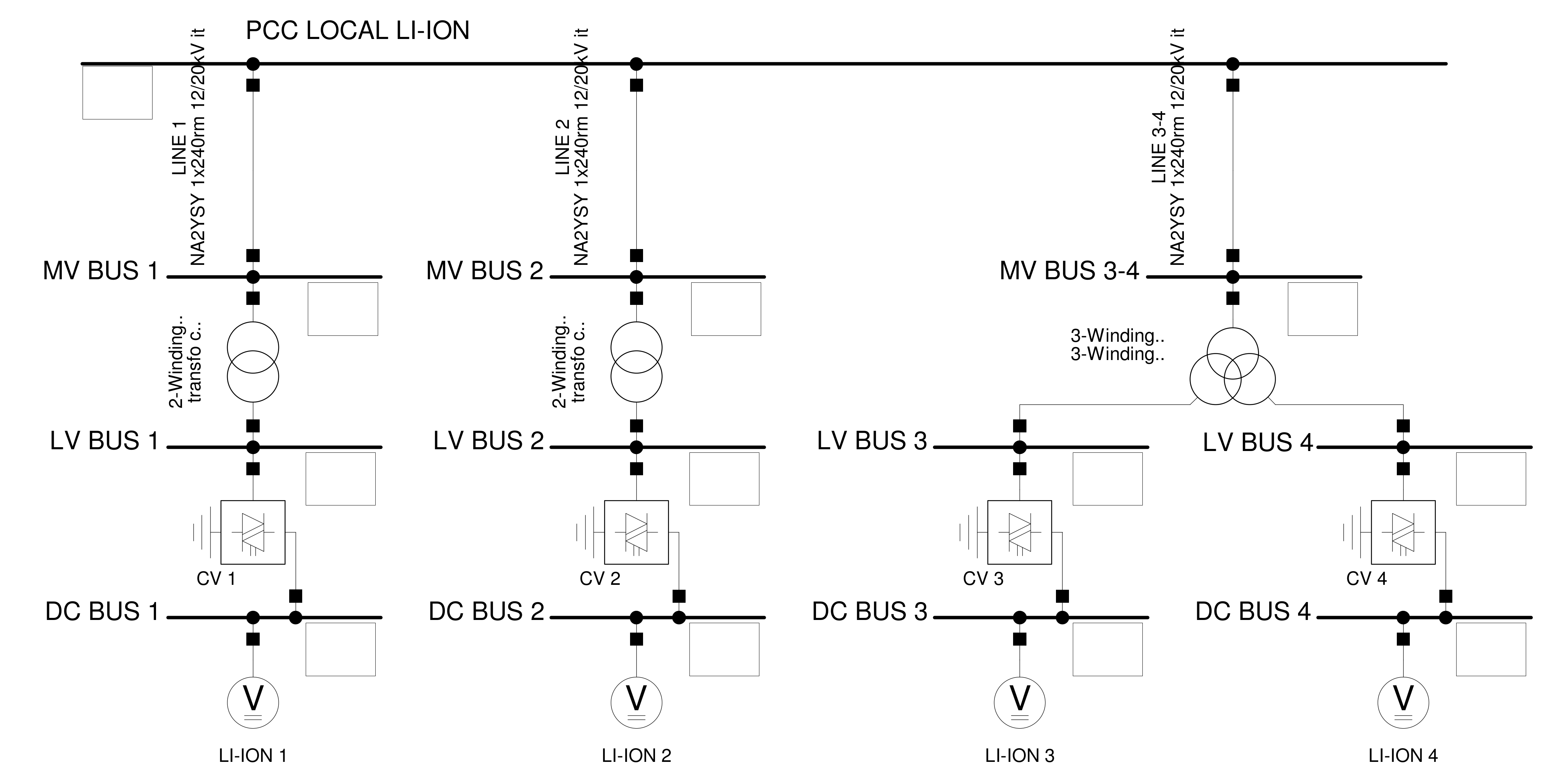
2. Island Grid-Connected Hybrid Power Plant

The archipelago of Guadeloupe is a French insular region and overseas department located in the eastern Caribbean Sea. Guadeloupe has a land area of 1628 ${\mathrm{km}}^2$ and had an estimated population of 449,089 in June 2018. The two main islands commonly referred to as the main island, Basse-Terre (848 ${\mathrm{km}}^2$) and Grande-Terre (586.7 ${\mathrm{km}}^2$), are separated by a narrow strait and are connected by bridges. The other three islands in the archipelago are the Department’s Dependencies: Les Saintes, Marie-Galante and La Désirade.

The Guadeloupe Archipelago is a Non-Interconnected Zone that must produce all the electricity it consumes, where Électricité de France (EDF) is a public utility (production, single buyer, transport, distribution and marketing) [35]. For this, submarine cables connect each of the islands to the loops of overhead lines covering Basse-Terre and Grande-Terre. The installed capacity of Guadeloupe’s electrical grid is of 556.46 MW. The archipelago is a territory almost totally dependent on thermal non-renewable sources (coal, diesel and combustion turbines), and $80\%$ of the electricity consumed comes from these fossil fuels.

However, in recent years, Guadeloupe has adopted renewable energies. In 2017, its electricity mix consisted of more than $20\%$ of renewable energy. Thus, apart from coal, diesel, and fuel, several renewable sources are used to produce electricity on the island territory: solar (photovoltaic), geothermal, wind, hydroelectric and biogas. For this, different projects have been developed in order to size and install renewable power plants in this territory, as shown in Figure 1 [36]. This paper proposes a study to assess and validate the operating of a new hybrid wind/storage power plant at a particular point of the Guadeloupe electric grid (Sainte-Rose).

Guadeloupe’s Electrical Grid Model

Guadeloupe’s PowerFactory model of electrical system shown in Figure 2 was implemented from the data presented in Reference [37]. The shaded area corresponds to the point of common coupling located within the Sainte-Rose node, where the HPP is connected.

Guadeloupe’s electrical grid has a 63 kV high voltage transmission system, consisting of two big loops of overhead lines. The first loop covering Basse-Terre is interconnected through the Jarry Nord and Jarry Sud substations with the second Grande-Terre’s loop, which is made up of 13 nodes that correspond to HTB/HTA (High Voltage B or HTB is the electrical voltages range from 50,000 volts (50 kV) to 400,000 volts (400 kV). High Voltage A or HTA (or Medium Voltage) can be between 1000 volts (1 kV) and 50,000 volts (50 kV). HTB and HTA represent the voltage domains for electricity networks in France.) substations, each comprising two 63/20 kV step down transformers connecting loads and, in most cases, also reactive compensation stations. While an additional node corresponding to the Jarry Nord generation site is considered, the generator sets located in the islands Les Saintes, Marie-Galante, and La Désirade are not part of this grid model.

The wind-BESS hybrid power plant is depicted Figure 3. The wind generation system comprises four 2 MW wind turbines with their respective converters and transformers. Meanwhile, the BESS consists of four storage units connected in parallel (1 MW/580 kWh capacity by unit), with their respective converters and transformers.

The hybrid power plant is connected through a point of common coupling located within the Sainte-Rose node, as can be seen in the grid’s PowerFactory model in Figure 4. As shown, the Sainte-Rose node comprises a 63 kV busbar connected to 63 kV/20 kV transformers and two 20 kV busbars (Terminals 1 and 2), and, at the same time, it is connected to the main busbars at the neighboring substations Bouillante and Baie-Mahault. Terminal 1 relies on a local load and serves as a point of common coupling for the HPP. Meanwhile, terminal 2 relies on a load and a static var system.

According to the data presented in Reference [37], $53\%$ of the load in Guadeloupe can be considered static, representing mainly home appliances. For the sake of simplicity, in the grid model implemented in this paper, all the loads were assumed to be static and invariant with respect to the frequency and voltage changes.

3. Formulation of the Problem

This section provides the problem formulation for the HPP’s optimal operating, which contains the objective function and technical and electrical constraints for the optimization problem. Given the nature of the wind-storage HPP, and the complexity of the revenue optimization problem dealt with, it seems appropriate to give priority to methods to find optimal solutions combined with control strategies handling the forecasting aspects.

According to the HPP’s characteristics, the EMS proposed should ensure the continuous power injection from the wind-storage HPP into the Sainte-Rose substation on the island’s electricity grid, according to the commitment profile generated on the basis of the wind forecast. Under those circumstances, the optimization problem consists of deciding on how to use the battery energy storage system (i.e., which part of the production is used to charge the BESS or how much power is to be discharged) as the WTs output instantly varies, to transfer to the island grid according to a committed generation schedule.

In addition, the disrespecting the accepted injection region above and below the commitment may lead to commitment failures (triggered by injection band overtakes lasting 60 s) that are associated with economic penalties. The proposed strategy aims at maximizing this profit and avoiding the occurrence of penalty conditions [38].

3.1. Power Dispatch Optimization

The aim of the Multi-objective EMS developed in this work is to ensure that the power is supplied to the main grid in a robust way and respecting the operating rules, while maximizing the plant’s profit. These operating rules are described below through objectives and constraints which define the EMS:

3.1.1. Objectives

• Power injection band respect: a tolerance region (injection band) is established on the basis of the injection schedule. This objective consists of minimizing the error difference between the power injected ($P_{INJ}$) and scheduled ($P_{SCHED}$), which is similar to attracting $P_{INJ}$ towards the center of the tolerance region.
• Favoring the BESS availability: this objective consists of seeking to reduce the occurrence of BESS unavailable conditions, so, during strong wind periods, it can be used to store power, and it can be discharged during weak wind periods.

3.1.2. Constraints

Several technical and electrical constraints should be considered for an optimal dispatch with respect to a day-ahead planning. These constraints include electrical and operational constraints of the HPP’s different components:

• Maximal power injection: an upper bound is defined for $P_{INJ}$ to reduce the overtakes of the band’s threshold.
• Rate of change of power injected: the speed of change of $P_{INJ}$ is limited in order to avoid abrupt changes in the power transferred towards the grid.
• State-of-charge: the BESS must be operated in accordance with the recommendations of the manufacturer in terms of depth-of-discharge and charging rates in order to optimize its lifespan.
• BESS maximum charge/discharge current: Considering the manufacturer’s recommendations, the BESS maximum continuous charge and discharge currents should be respected.

In order to guarantee the reliability and stability of the microgrid, operating rules corresponding to system objectives and constraints need to be established.

4. Mathematical Modeling of the HPP Subsystems

In this paper, a PowerFactory/MATLAB co-simulation methodology was carried out in order to assess the impact of a wind-storage hybrid power plant, injecting power into one of the HTA busbars of the Sainte-Rose substation. Both the hybrid power plant and a basic EMS are considered being part of the system implemented in PowerFactory. The grid model is then validated through simulation by comparison with respect to some literature available data.

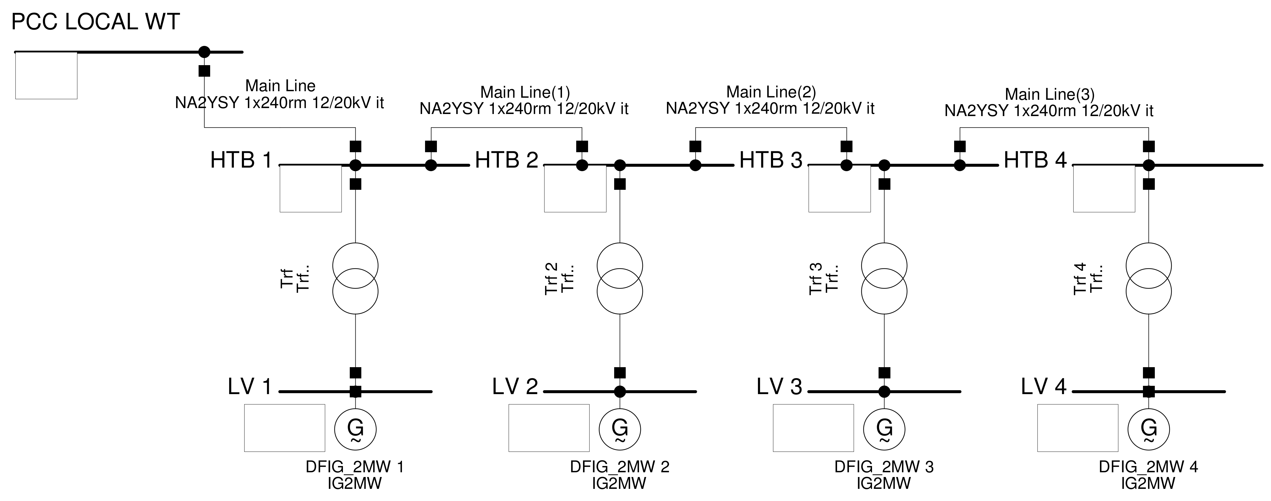
4.1. Wind Generation System Modeling and Validation

The wind generation system’s single line diagram described by PowerFactory software is depicted in Figure 5. As shown, this system consists of four 2 MW WTs based on Doubly Fed Induction Generators (DFIG) with their respective rotor-side converters (RSC) and transformers.

The DFIG (electrical component) is modeled through the Pulse-Width Modulation (PWM) converter, which allows for flexible and fast control of the machine by modifying the magnitude and phase of the output voltage on the rotor-side [39,40].

The power curve of the wind turbine modeled is displayed in Figure 6. This curve presents the steady-state electrical power obtained from simulation for wind speeds ranging from start-up wind speed (3 m/s) up to shut-down speed (29 m/s). In this operating mode, in order to get a constant power output above nominal speed, the pitch angle was adjusted accordingly to control the stall effect. On the other hand, between start-up speed and nominal speed (12 m/s), the power output is maximized.

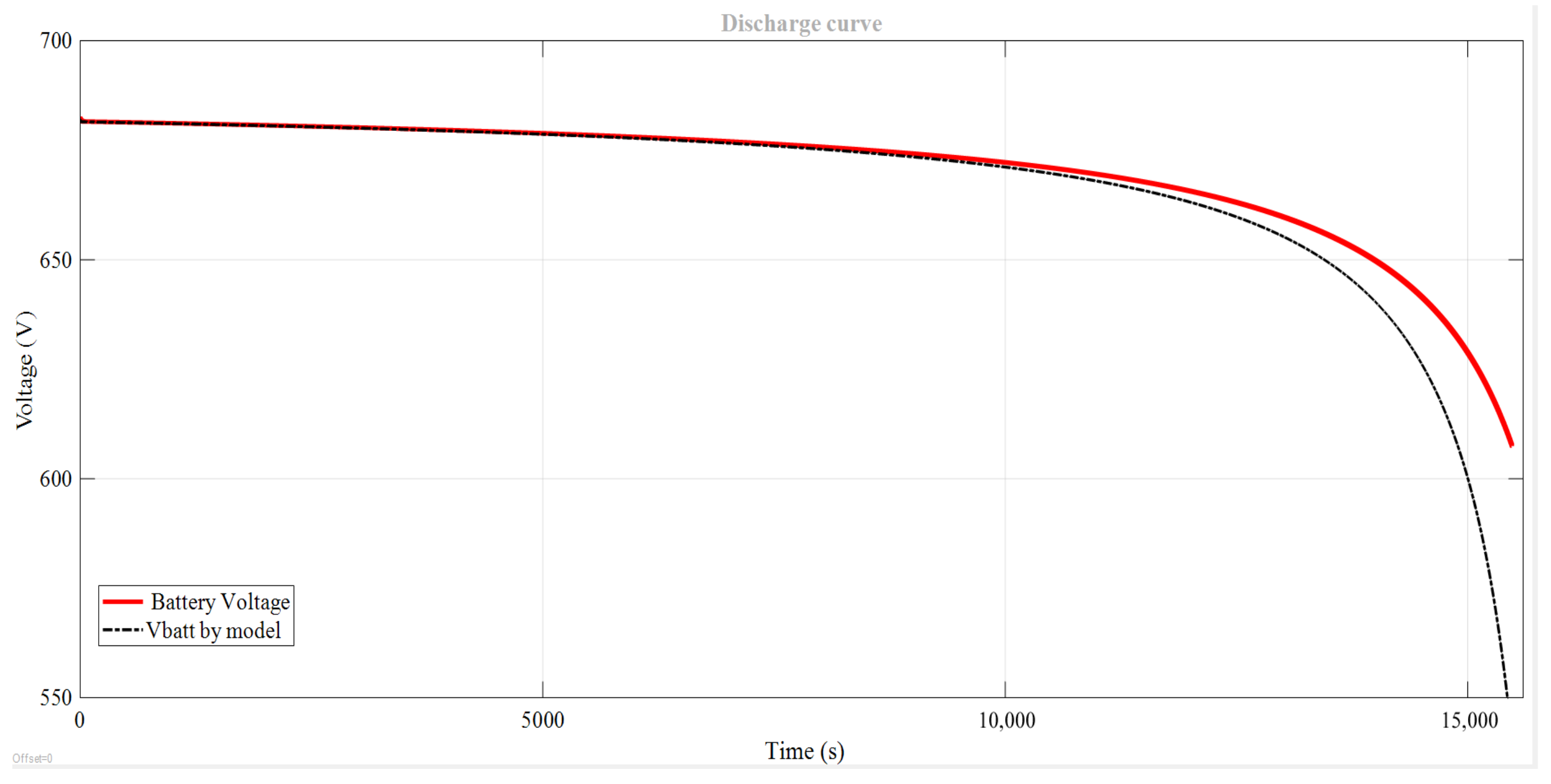
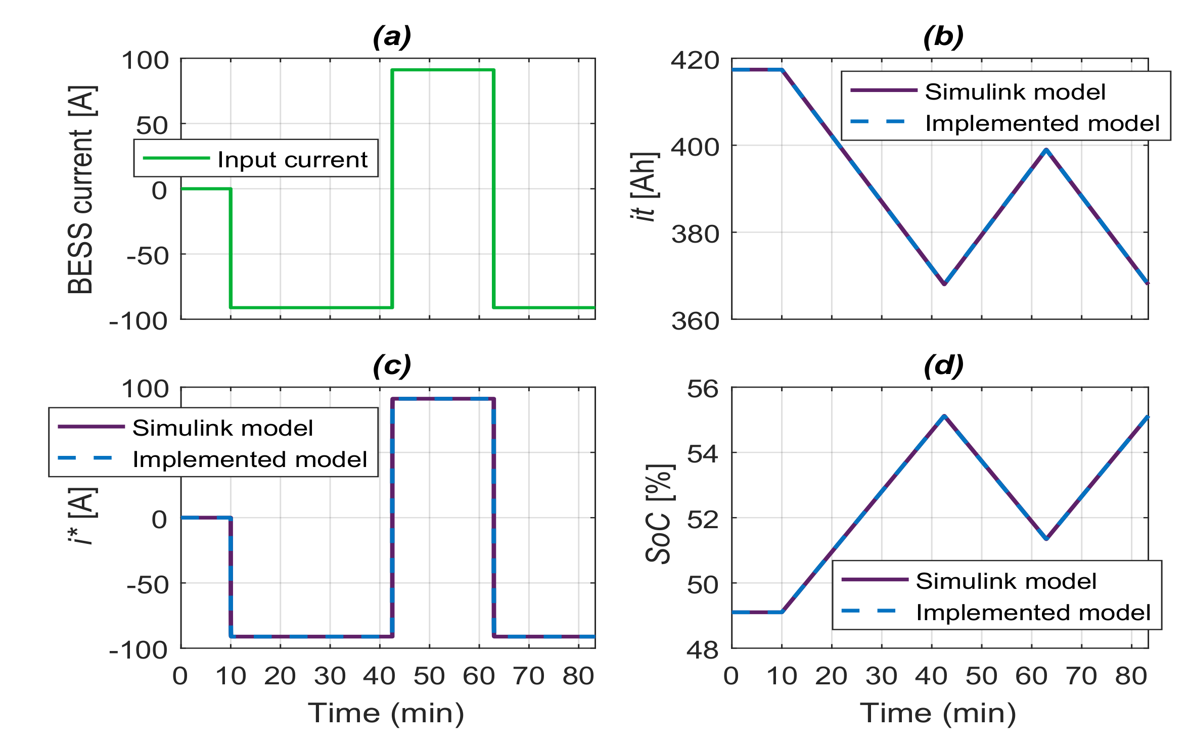
4.2. Li-ION Battery Modeling and Validation

The storage system is the main degree of freedom of the HPP management problem dealt with in the present work. Two models of the BESS are implemented using the Tremblay model equations [41]. The first is a nonlinear plant model, and the second, a linear state-space model model for control. The modeling is inspired by the commercial storage solution Intensium Max 20M (IM20M) of Saft. While the BESS comprises four parallel IM20M units, the validation focuses on a single IM20M battery.

The Tremblay model describes the output voltage of a cell as a function of the capacity in ampere hours (Ah) that have been obtained from it [41]. According to this model, the battery cell is represented by a voltage source with variable magnitude in series with a resistance.

Figure 7 shows the battery discharge curves at constant current obtained by the proposed model, compared with the SimPowerSystems battery model available on the MATLAB/Simulink [41,42]. For that, the discharge current considered was $I_{nom}/38$ (A), whereas the minimum voltage for the battery was 609 (V) [38]. The model presents a linear section that indicates the charge that can be extracted from the battery before the voltage drop below its nominal value ($V_{nom}$). Within this region, the state-of-charge lies between $20\%$ and $80\%$ of the battery’s nominal capacity.

Figure 8 represents the discharge model. An identification method for fitting the resulting discharge curve to the curve in the battery manufacturer’s data-sheet was presented by the authors in Reference [43]. The method was used in Reference [44] to obtain the parameter values of the Saft’s VL41M cell, single unit of the IM20M, by comparison with discharge curve in the battery manufacturer’s data-sheet.

The method applies optimization techniques to find the values of the X vector, subject to $X^{min}$ and $X^{max}$ as follows:

$$\begin{array}{c}\hfill \begin{array}{cc}\hfill X& =\left[E_0\overline{A}\overline{B}RK\right]\hfill \\ \hfill X^{min}& =\left[E_0^{min}{\overline{A}}^{min}{\overline{B}}^{min}{R}^{min}{K}^{min}\right]\hfill \\ \hfill X^{max}& =\left[E_0^{max}{\overline{A}}^{max}{\overline{B}}^{max}{R}^{max}{K}^{max}\right]\hfill \end{array},\end{array}$$

(1)

where $E_0$ is the battery constant voltage (V), R represents the internal resistance of the battery $(\Omega )$, $\overline{A}$ is the exponential zone amplitude (V), $\overline{B}$ is the exponential zone time constant inverse $\left(A{h}^{-1}\right)$, and K represents the polarization resistances constant. These obtained values allow the following cost function to be minimized:

$$f_{obj}\left(X\right)=\sqrt{\sum _{i=1}^{i=n}\sum _{Q=0}^{Q=Q_{nom}}{(V_{mes}(Q,I_i)-V(Q,I_i))}^2},$$

(2)

where $I_i=I_1,...,I_n$ represents the discharge currents, which allows that the quadratic error among the manufacturer’s voltage $V_{mes}$ and the model estimations V to be minimized.

Table 1. Cell parameters values.

Symbol	Description	Unit	Value
$V_{full}$	Fully charged voltage	V	3.95
$V_{nom}$	Nominal voltage	V	3.6
$V_{exp}$	Exponential voltage	V	3.9
$Q_{nom}$	Nominal capacity	Ah	39
$Q_{max}$	Maximum cell capacity	Ah	41
$Q_{exp}$	Exponential capacity	Ah	1
I	Nominal discharge current	A	13.67
$V_{chlim}$	Cell charge voltage limit	V	4
$V_{dchlim}$	Cell cut-off voltage	V	2.7

lists the parameters identified for the VL41M battery.

The IM20M comprises 20 parallel branches and 174 series of the Saft’s VL41M cell (3.6 V and 41 Ah) and allows a nominal power of 1 MW for a capacity of 580 kWh. The Tremblay parameters values of the VL41M cell used in the implementation of the nonlinear model of the battery stack, are: $E_0=3.24$ V, $R=0.002\Omega$, $K=1.04\times {10}^{-4}$ V/Ah, $\overline{A}=0.75$ V, and $\overline{B}=0.034$${\mathrm{Ah}}^{(-1)}$ [44]. For validation, the model response to a current input signal is compared to the response of the battery block of Simulink, also configured to represent the IM20M (Figure 9a). Table 1 presents the values used to configure the Simulink battery. An initial state-of-charge of $50\%$ is chosen for the test, and the battery response times are set at 1.8 s, according to the battery’s specification. Figure 9b–d show the signals obtained for the states $it$, $i^{*}$ and $SoC$.

In turn, Figure 10 depicts the relative errors as percentages obtained when the implemented model is compared to the Simulink battery block.

The errors in the model for the signals $it$ and $SoC$ are close to zero (Figure 10a,c). Meanwhile, Figure 10b reveals an error caused by a delay between the $i^{*}$ signals obtained. Error peaks take place when the input current changes. However, for the control objectives of the EMS, these errors would be compensated by the controller as will be seen in the next section.

In an additional test, the initial state-of-charge was set at $100\%$, and the minimum and maximum $SoC$ limits, at 0 and $100\%$. Figure 11a presents the discharge of the 1 MW/580 kWh storage system obtained from the nonlinear model in MATLAB. Furthermore, the power reference was defined to withdraw 580 kWh from the battery during 1 h. As can be seen in Figure 11b, the power followed the reference until the $SoC$ reached $0\%$ after 52 min. The validation of a standalone storage unit allows confirming that this storage model is suitable for implementation in the hybrid plant model in the PowerFactory environment.

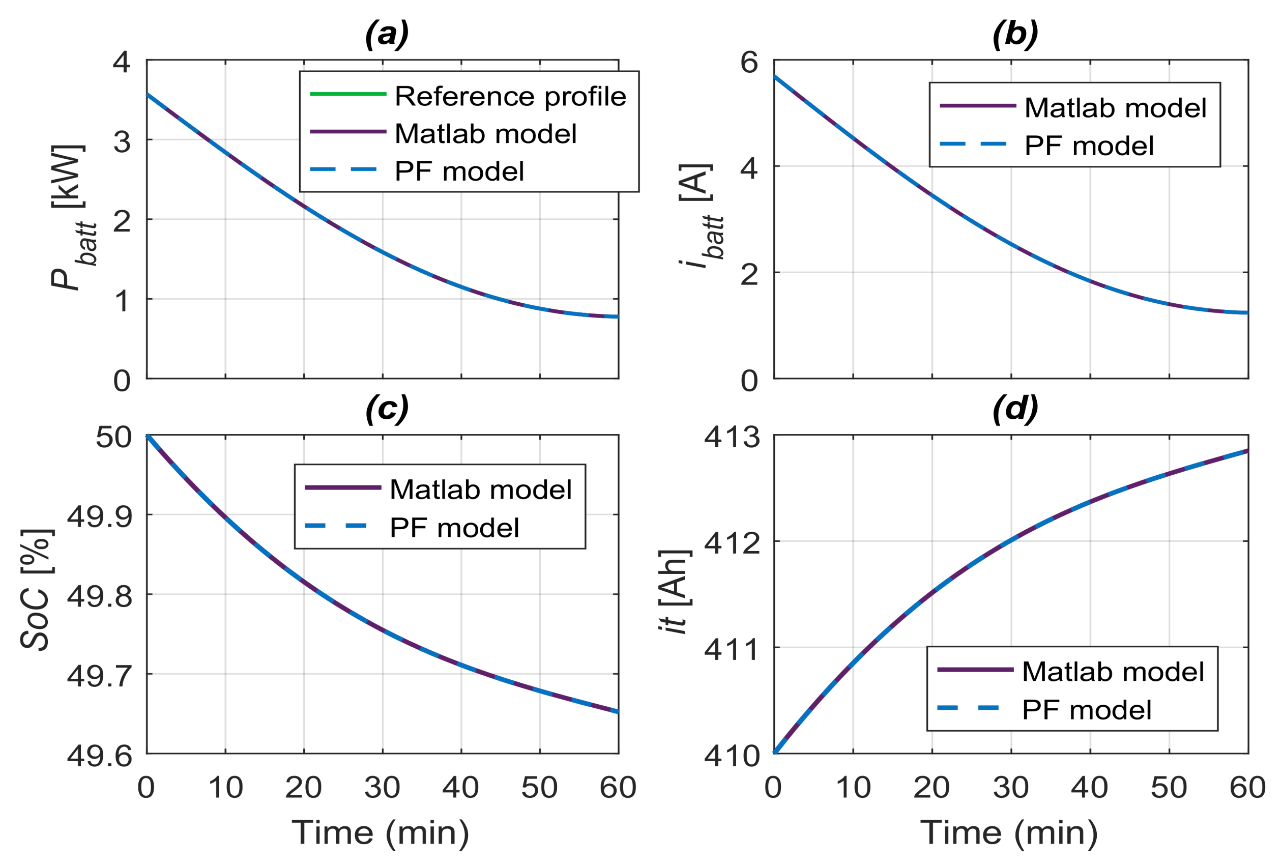
PowerFactory Model Validation

The PowerFactory BESS model (i.e., the controlled system model) is implemented as a standalone storage unit containing a DPL (DIgSILENT Programming Language) script with the Tremblay model equations and parameters to represent the IM20M battery.

To validate it, a power reference profile of 1-h duration is imposed on both the Simulink battery block and PowerFactory nonlinear BESS model.

The validation test results are presented in Figure 12. Figure 12a shows the reference power profile is followed by the battery power signals obtained from the two battery models. The resulting BESS current, state-of-charge ($SoC$), and integral current ($it$) signals are presented in Figure 12b–d. The state-of-charge limits are set at $20\%$ and $80\%$. A sampling time of 1 s was used in the simulations. As can be seen, the power signals are superposed, indicating the model proposed can be used in the control strategy.

Figure 13 presents the BESS implemented in PowerFactory. It comprises 4 Li-ION IM20M storage units, as well as their respective converters, transformers, busbars, and underground lines. This model will be coupled with the wind generation system to complete the HPP representation.

4.3. Storage System model for the MPC Strategy

A linear model of the storage system is required by the MPC strategy to generate optimal control actions. The proposed model should meet two conditions: to capture the dominant and important dynamics of the system, and also to remain simple enough to allow the optimization problem to be solved [45]. With this aim, a discrete-time state-space representation of the storage system model is given by the next equations set:

$$\begin{array}{ccc}\hfill i_t(k+1)& =& i_t\left(k\right)+{▵}_t{i}_{BESS}\left(k\right)\hfill \\ \hfill i^{*}(k+1)& =& (1-\alpha )i^{*}\left(k\right)+\alpha i_{BESS}\left(k\right)\hfill \\ \hfill SoC(k+1)& =& 100\left(1-\frac{i_t\left(k\right)}{Q}\right),\hfill \end{array}$$

(3)

where $i_{BESS}$ is the battery current (model input), $\alpha$ is a mitigating factor, and ${\Delta }_t$ represents the simulation step time. In addition, $k+1$ refers to the timestep one sample interval after the current timestep k. Equation (3) describes the BESS model used to represent the dynamic of the storage system extracted capacity $i_t$, filtered current $i^{*}$, and state-of-charge $SoC$. The model is valid for $SoC$ values within $20\%$ and $80\%$. The model’s output vector $y\left(k\right)$ contains the variables to optimize:

$$y\left(k\right)={\left[i^{*}\left(k\right)Soc\left(k\right)\right]}^T.$$

(4)

The HPP linear model for control is based on the BESS model and considers the power of the Wind Energy Conversion System (WECS) output ($P_{WECS}$) added to the battery power ($P_{BESS}$), allowing the power injected into the grid ($P_{INJ}$) to be obtained according to:

$$P_{INJ}=P_{WECS}+P_{BESS}.$$

(5)

Figure 14 shows the hybrid power plant model in which outputs are the predictions of $i^{*}$, $SoC$, $P_{BESS}$ and $P_{INJ}$ at the sampling rate $k+1$. Under those circumstances, $v_{BESS}$ is the storage system voltage, considered a measurable variable and available at every calculation step.

The battery power can be computed from the measured voltage and the filtered current as:

$$P_{BESS}=v_{BESS}·i^{*},$$

(6)

where $P_{BESS}$ is negative in case of discharge and positive in charge. The HPP linear model for control is then validated via PowerFactory/MATLAB simulations.

In Figure 15, the signals corresponding to the state variables are presented, as well as the battery power obtained in both cases. Figure 15a–c present the integral current, the filtered current, and the state-of-charge, respectively. The integral current and state-of-charge resulting from the linear model behave as those obtained from the nonlinear modeling (relative errors smaller than $0.2\%$ and $0.3\%$, respectively). While the filtered current plot (Figure 15b) shows an error smaller than $10\%$ during $97\%$ of the time. Some peaks are presented during the reference changes. In Figure 15d, the linear model storage system’s active power was calculated as $v_{\left(BESS\right)}·i^{*}$ according to Equation (6). The voltage signals involved being the same, it can be observed that $i^{*}$ introduced a filter effect reducing the oscillations in the estimation of the active power done through the linear model. Figure 16 presents the input and output signals for the controller based on the storage system linear model.

As can be seen, the active power reference profile $P_{BES{S}_{ref}}$ is obtained from the commitment generation schedule $P_{SCHED}$ and the output power of the wind energy system $P_{WECS}$, as:

$$P_{BES{S}_{ref}}=P_{SCHED}-P_{WECS},$$

(7)

where the signal $P_{SCHED}$ can be understood as the reference for $P_{INJ}$, i.e., the power injected into the main grid. Then, dividing $P_{BES{S}_{ref}}$ by the battery measured voltage $v_{BESS}$ gives the reference current signal $i_{BES{S}_{ref}}$, which is defined as the decision variable u.

5. MPC Control Strategy

Model Predictive Control (MPC), refers to a family of control methods which use the controlled system model to obtain a control signal by minimizing an user-defined objective function [45]. MPC allows the incorporation of constraints as part of the control design requirements, enabling their systematic handling. Compared to classical linear unconstrained methodologies, such as PID techniques, MPC has proven to produce much better results as it allows the systems to be operated near their constraint boundaries [46].

MPC is an intuitive strategy which consists of planning over a finite time window (called prediction window) the future control actions that would lead to the desired outcome. For that, the control signals are calculated by optimizing a criterion to keep the process as close as possible to the reference trajectory via a cost function [45].

In this study, the MPC strategy uses the current state information of the Li-ION BESS, as well as future references of the control objectives, to determine the control actions optimizing the power injected into the grid. An assumption done consists of considering that the control inputs, received at the beginning of the prediction window, remain constant over that time window.

5.1. Energy Management with Respect to a Day-Ahead Power Injection Planning

The energy management problem of ensuring the wind-BESS storage HPP supply a grid service that consists of complying with a day-ahead power injection schedule is dealt with in the present work. Model predictive control and quadratic programming optimization are combined to step-wisely generate optimum solutions while considering forecasts, instant power generation and measures of the current system state.

5.1.1. Operational Objectives

The aim of the EMS developed is to ensure that the power supplied to the grid by the wind-storage HPP respects the operating rules while maximizing the plant’s profit. Below are described the functioning objectives taken into consideration during the strategy design are described:

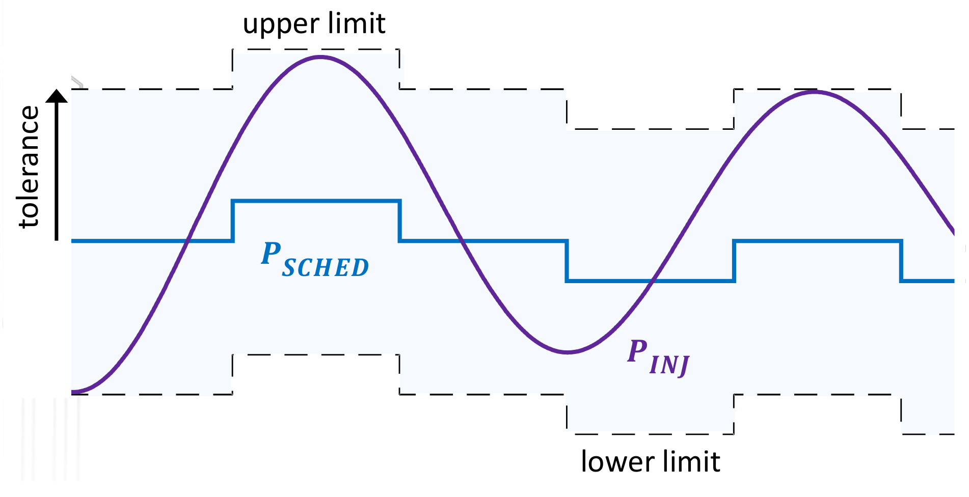
• Forecasts and power injection band: the plant operation is based on 24 h of wind speed forecasts for the period 0:00–23:59 h for day D+1 (i.e., the next day, when the actual production is taking place). A scheduling algorithm represents the forecasted injection in the form of a half-hourly stepped profile.
  Such a profile is taken here as the day-ahead power injection schedule ($P_{SCHED}$). The injection band represented in Figure 17 is built from $P_{SCHED}$ and established taking into consideration the fact that the energy storage system must be controlled so that the 30-min duration scheduled injection steps can be met. During the first year of operating the HPP, the BESS should allow the respect a tolerance region of $25\%$ of the installed power $P_{MAX}$, above and below the scheduled injection. The band will be narrowed down to $20\%$ the second year and to $15\%$ from the third year.
  In this paper, the distance between $P_{SCHED}$ and the bounds of the band is called injection tolerance and is set at $25\%$ of the installed capacity of the wind farm, $P_{MAX}$, as required in the first year of the project.
• Favoring the BESS availability: A reference is defined at a $50\%$$SoC$. Seeking to keep the stored power at a half of BESS capacity means finding the right trade-off between charging or discharging the BESS, avoiding if possible the $SoC$ boundaries.
• Plant revenues and penalty system: Plant revenues are determined via a penalty system. Power injections with excursions of 60 consecutive seconds outside the limits are penalized with non-payment of the power supplied to the grid for the next 10 min. The plant revenue can then be calculated considering the energy selling price ($SPin/cperkWh$) as:

  $$PR=\sum _{t=0}^{sim.time}{P}_{INJ}\left(t\right)\times SP\left(t\right)\times \partial \left(t\right),$$

  (8)

  where

  $$\partial \left(t\right)=\left\{\begin{array}{cc}0& whenapenaltyconditionisactive\\ 1& inothercases\end{array}.\right.$$

5.1.2. Operational and Technical Constraints

• Maximal power injection:$P_{INJ}$ is constrained by a limit equal to the band upper boundary. With this, when searching for optimal solutions, the algorithm will not consider possible solutions that drive the power injection above the mentioned boundary. In line with this, $P_{INJ}^{max}$, the upper limit for the power transfer, is computed according to the evolution of the commitment profile, as follows:

  $$P_{INJ}^{max}=P_{SCHED}+tol·P_{MAX},$$

  (9)

  with $25\%tolerance$, the term $tol·P_{MAX}$ gives $2MW$. Conversely, the minimum injection occurs when the WTs are not generating power and the BESS is not delivering power. To avoid penalties, rather than setting constraints on both the upper and lower injection band limits, the constraint $P_{INJ}^{max}$ is placed on the band ceiling $P_{INJ}\le P_{INJ}^{max}$. This way, instead of allowing injections greater than the upper limit, extra available power can be used to charge the storage system. This constraint was defined through the state variable $i^{*}$, which is a controlled output.
• Rate of change of power injected: according to the contractual specifications of the HPP operation, the speed at which $P_{INJ}$ varies (in MW/s) must be limited so that: (1), the time it takes to go from 0 to $P_{MAX}$ is in the range (5–30 min), and (2), the time it takes to go from $P_{MAX}$ to 0 is in the range (1–10 min). However, one single range of (1–5 min) is considered for both, positive and negative power injection variations. Moreover, as the constrained variable is the controller model input, $u=i_{BESS}$, the limits are expressed in terms of current:

  $$\begin{array}{c}\hfill \frac{(P_{SCHED}+tol)/300}{v_{BESS}}\left[\frac{W/s}{V}\right]Lowerlimit\\ \hfill \frac{(P_{SCHED}+tol)/60}{v_{BESS}}\left[\frac{W/s}{V}\right]Upperlimit,\end{array}$$

  (10)

  where the use of the absolute value indicates that the equation is valid for both going from $P_{MAX}$ to 0, and vice versa. As noted, the lower limit is associated with the larger time in the range (5 min or 300 s), whereas the upper limit is related to the case where the passing takes place in 1 min (60 s). The reason for this is a shorter passing time implies a steeper slope, or a bigger rate of change limit. Making the limits for the rate of change of $u=i_{BESS}$, in inequality form, gives:

  $$\frac{1}{300}·\frac{(P_{SCHED}+tol)}{v_{BESS}}\le \frac{du}{dt}\le \frac{1}{60}·\frac{(P_{SCHED}+tol)}{v_{BESS}},$$

  (11)

  which are constraints for upward and downward steps of $d{P}_{INJ}/dt$. In other words, these constraints limit the speed of change of $P_{INJ}$ to avoid abrupt changes in the power transferred towards the grid.
• State-of-charge: the BESS must be operated with $60\%$ depth-of-discharge maximal in accordance with the manufacturer’s recommendation. In addition, the linear model is valid if the $SoC$ is within $20\%$ and $80\%$ Hence, the $SoC$ is limited to the aforementioned range.
• BESS maximum charge/discharge currents: Considering the sign convention defined for BESS, the maximum continuous charge and discharge currents are, respectively, 3280 A and $-6400$ A.

The extra power obtained by forbidding power injection levels beyond $P_{INJ}^{max}$ is rendered available for charging the BESS. The extra power obtained by avoiding injections beyond the band ceiling can be used to prevent penalties due to the overshoot of the lower boundary. In addition, placing a constraint on the band floor could make the controller diverge in the case of injection levels below the lower boundary, so such limitations are avoided.

Table 2. Limitations assigned to the constraints.

Parameter	Description	Unit	Value
$i^{*max}$	Filtered current upper bound	A	$\frac{P_{SCHED}+tol}{v_{BESS}}$
$u^{min}$	Control amplitude lower bound	A	−6400
$u^{max}$	Control amplitude upper bound	A	3280
$So{C}^{min}$	State-of-charge upper limitation	%	20
$So{C}^{max}$	State-of-charge lower limitation	%	80
$\frac{d{u}^{min}}{dt}$	Control actions rate of change lower bound	A/s	$-\frac{1}{300}·\frac{P_{SCHED}+tol}{v_{BESS}}$
$\frac{d{u}^{max}}{dt}$	Control actions rate of change upper bound	A/s	$\frac{1}{60}·\frac{P_{SCHED}+tol}{v_{BESS}}$

recapitulates the constraints limits established.

5.2. Prediction and Optimization Strategy

The proposed control and optimization strategy generates a control signal $\tilde{u}$ optimizing stepwise the quadratic cost function described in Equation (12), over a prediction horizon of size $Np$. To do that, it requires future references and current state measurements of the BESS.

$$\begin{array}{cc}\hfill \Gamma \left(k\right)=\sum _{i=1}^{Np}& \left\{{\lambda }_1\parallel P_{INJ}-P_{INJref}{\parallel }^2+{\lambda }_2{\parallel SoC-So{C}_{ref}\parallel }^2+\right.\hfill \\ & \left.Q_u{\parallel \tilde{u}\parallel }^2\right\}.\hfill \end{array}$$

(12)

In Equation (12), ${\lambda }_1$ and ${\lambda }_2$ are the control objective weights. $P_{INJref}$ and $So{C}_{ref}$ are the references established for the transfer of power to the power grid and for the SoC evolution. $Q_u\in {\mathbb{R}}^{n_u\times n_u}$ is a symmetric positive definite matrix for weighting and adjusting the control effort of the inputs, with $n_u$ the number of inputs. The control sequence $\tilde{u}$ consists of elements $u(k+i-1)$ with $i\in \left\{1,\cdots ,Np\right\}$:

$$\tilde{u}\left(k\right)=\left(\begin{array}{c}u\left(k\right)\\ u(k+1)\\ ⋮\\ u(k+Np-1)\end{array}\right),$$

(13)

for a total of $N_p$ possible future control actions. Finally, $\Gamma$ can be interpreted as the cost obtained by the evaluation of the future control actions function $\tilde{u}$ using the future references $P_{INJref}$ and $So{C}_{ref}$ and the present system state $x\left(k\right)$ within the time horizon $[k,k+N_p]$.

The cost function described in Equation (12) was derived based on MPC control law while considering the control objectives. An appropriate optimization algorithm is now required to reduce future errors based on such a quadratic function and in the presence of linear constraints. For that, the parametric prediction approach presented in Reference [47] is used. The approach is compatible with the quadratic programming solver provided by MATLAB’s optimization toolbox (quadprog). This solver finds the minimum $\mathrm{x}$ for problems specified by the following expression [48]:

$$\begin{array}{cc}\hfill \mathrm{minimize}& \frac{1}{2}{\mathrm{x}}^T\mathbf{H}\mathrm{x}+{\mathrm{f}}^T\mathrm{x}\hfill \\ \hfill \mathrm{subject}\mathrm{to}& {\mathbf{A}}_{ineq}\mathrm{x}\le {\mathrm{b}}_{ineq}\hfill \\ \hfill & {\mathbf{A}}_{eq}\mathrm{x}={\mathrm{b}}_{eq}\hfill \\ \hfill & \mathrm{l}\le \mathrm{x}\le \mathrm{u},\hfill \end{array}$$

(14)

where $\mathbf{H}$ and f are required, whereas the other parameters are optional. ${\mathbf{A}}_{ineq}$ and ${\mathbf{B}}_{ineq}$ allow inequality constraints to be defined, whilst ${\mathbf{A}}_{eq}$ and ${\mathbf{B}}_{eq}$ allow equality constraints to be defined. In the strategy applied, the quadprog function is used with the input variables $\mathbf{H}$, f, ${\mathbf{A}}_{ineq}$, and ${\mathbf{B}}_{ineq}$.

$\mathbf{H}$ is calculated based on the system’s matrices (from the state-space model), and the weights ${\lambda }_1$, ${\lambda }_2$, and $Q_u$. f depends on the system, on the weights ${\lambda }_1$ and ${\lambda }_2$, on the present state vector $x\left(k\right)$, and on the future references $P_{SCHED}(k+i)$ and $So{C}_{ref}(k+i)$, $i\in \left\{1,\cdots ,Np\right\}$. ${\mathbf{A}}_{ineq}$ and ${\mathbf{B}}_{ineq}$ are matrices containing information on the trajectory’s constraints. The first depends only on the system, whereas the latter, in the present state, depends on the limits assigned to the constraints and on the system.

The cost function is convex, i.e., it has a global optimum, if the Hessian matrix $\mathbf{H}$ is definite positive. The last term in Equation (12) that takes into consideration the control effort, ensuring the positive definiteness of $\mathbf{H}$.

To use MPC strategy with the quadprog solver, the prediction information given to the optimizer must be defined by the matrices $\mathbf{H},{\mathbf{A}}_{ineq},{\mathbf{A}}_{eq}$ and vectors $\mathrm{f},{\mathrm{b}}_{ineq},{\mathrm{b}}_{eq}$. The idea is feeding at every time step a prediction-based cost function while reducing computations taking place online as much as possible. This procedure enables solutions to be obtained at every instant. Figure 18 shows a closed-loop, including a model predictive control with quadratic programming (MPC/QP) composed of prediction and optimization stages used to control the hybrid plant.

At this stage, the optimization subroutine must receive at every time slot the input ($\mathbf{H},\mathrm{f}$) with the prediction information. Here, $\mathbf{H}$ is considered constant, whereas value $\mathrm{f}$ is updated at every calculation step. Future references in Figure 18 and current state measurements appear in the controller input. Furthermore, the first element from the control action optimal sequence is sent to the BESS to indirectly control the power transferred to the grid $P_{INJ}$.

5.3. Economic Optimization of the HPP Operation with Respect to a 24-H Commitment Profile

The aim of the proposed algorithm is to maximize the plant’s revenues by minimizing commitment failures. As more transferred energy means an increased plant turnover, the algorithm settings allowing to act on the amount of power injected into the main grid need to be adjusted. Namely, two parameters can be used to optimize the HPP operation.

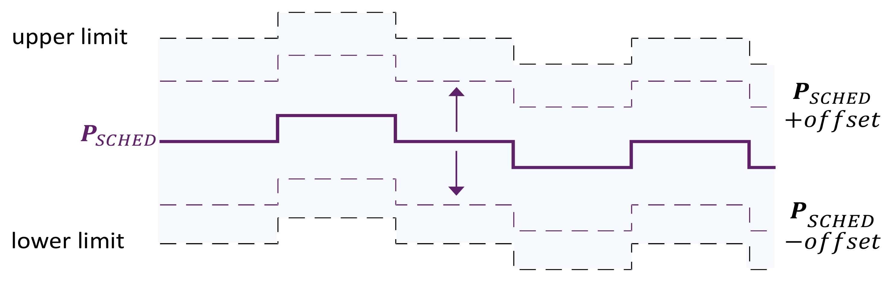
• Weights of the optimization objectives: Settings that can be modified to influence the power injection are the relative weights of the optimization objectives and the commitment $P_{SCHED}$, through the addition of a vertical offset, as represented in Figure 19. Such an offset that can be positive or negative.
• Other strategies may focus on maximizing of the energy stored in ESS or on keeping the control actions to a minimum, while the commitment failures are minimized.

5.4. Energy Management System KPIs

In order to evaluate the proposed Day-Ahead Energy Management System, several Key Performance Indicators (KPIs) have been established for monitoring the good wind-storage HPP performance. In projects related to smart grid development in isolated energy systems, this evaluation allows a quantitative assessment, by adopting representative KPIs, providing the relevant stakeholders with a useful comparison between the proposed solutions [49].

The KPIs chosen in this work are not only performance indicators assessing the characteristics of the technology solution proposed but also to identify the margins available, towards optimizing the smart and efficient operating of a grid in a cost-effective way. Here, the functioning goals and restrictions of the wind-storage HPP were needed for the KPIs’ definition.

• Commitment Failure (CF %): The optimization problem consists of deciding on how the storage system is used (i.e., which part of the production is used to charge the BESS or how much power is to be discharged) as the wind turbines output instantly varies, to inject power into the island grid respecting a committed generation schedule. Then, the commitment profile is generated based on day-ahead forecast data. In addition, the disrespecting of the accepted injection region above and below the commitment may lead to commitment failures (triggered by injection band overtakes lasting 60 s) that are associated with economic penalties. Then, the commitment failures are calculated as the percentage of the time during which the penalty condition was active, or:

  $$CF\%=100\frac{Numberofminuteswithpenaltytriggered}{Totaltesttimeinminutes}.$$

  (15)
• Curtailment Power ($P_{curt}\%$): In some cases, losses can be presented due to a power overproduction by the wind turbines while the BESS is fully charged. This KPI allows these losses to be monitored and the effectiveness of the EMS proposed to be tested, which handles the way in which battery’s cycles respect the day-ahead commitment at the same time as minimizing these losses. To obtain this KPI, whenever $P_{WECS}>P_{SCHED}+tol$, the lost power due to curtailment is calculated as:

  $$(if{P}_{WECS}>bandceiling):P_{curt}=P_{WECS}-(P_{SCHED}+tol).$$

  (16)
  By considering the dissipated power, Equation (5) could be rewritten as:

  $$P_{INJ}+P_{curt}=P_{WECS}+P_{BESS},$$

  (17)

  where the curtailed power is considered lost power. Then, the percentage of the power produced that was curtailed is obtained from:

  $$P_{curt}\%=100\frac{P_{curt}}{P_{WECS}}.$$

  (18)
• Not Supplied Power:
  Whenever a commitment failure has been triggered, the power not billed is calculated as:

  $$(ifCF=ON):P_{notbilled}=P_{WECS}+P_{BESS}.$$

  (19)
  This means that the total remunerated injection is:

  $$P_{INJ}=P_{WECS}+P_{BESS}-P_{curt}-P_{notbilled}.$$

  (20)
  The energy injected ($E_{INJ}$ in MWh) is computed from the injected power by considering the time. Finally, the non-remunerated production (due to commitment failures) as a percentage is obtained by:

  $$P_{notbilled}\%=100\frac{P_{notbilled}}{P_{WECS}}.$$

  (21)
• Counting Battery Cycles: the lifetime of a battery is influenced by several factors, including the number of charge-discharge cycles. For this reason, correctly estimating battery deterioration is needed to establish an adequate operating region to maximize their lifetime, as well as to obtain the highest returns on investment. Thus, in order to keep track of the storage system’s use, partial charging and discharging cycles are considered as follows:

  $$\begin{array}{c}chg=chg+▵SoC,if▵SoC>0\\ dchg=dchg+▵SoC,if▵SoC<0\end{array},$$

  (22)

  where $chg$ and $dchg$ are percentages (%) obtained from adding all the positive and negative changes in the $SoC$, respectively. Those changes ($▵SoC$) are given by:

  $$▵SoC\left(k\right)=SoC\left(k\right)-SoC(k-1).$$

  (23)
  Then, the storage system cycles (at $60\%$ DoD) are computed as:

  $$BES{S}_{cycles}=BES{S}_{cycles}+(chg+dchg)/120,$$

  (24)

  meaning that, when each $chg$ and $dchg$ is equal to $60\%$, $BES{S}_{cycles}$ are incremented by one cycle. The method used to count the cycles here is based on the approach introduced in Reference [50].

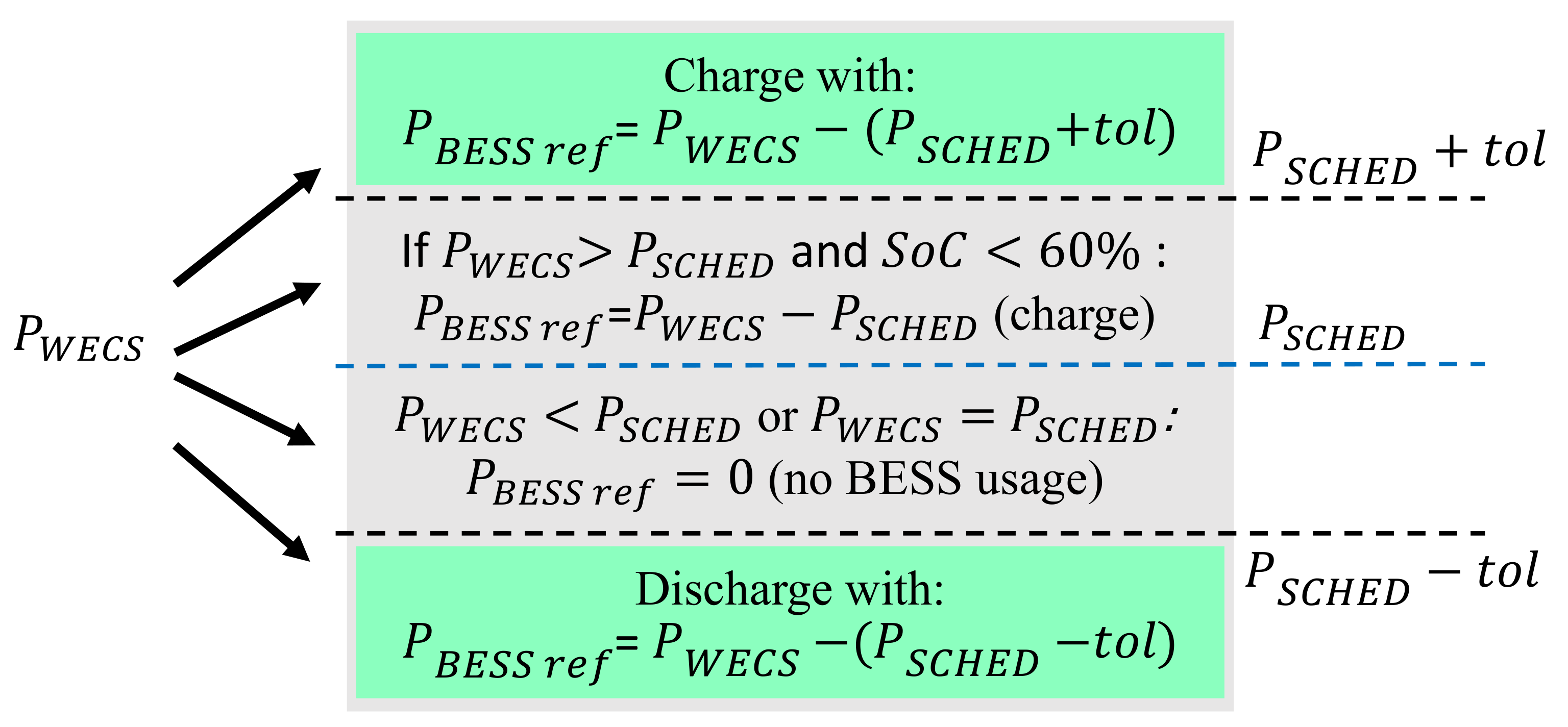
5.5. Rule-Based Strategy Operation

The rule-based that was taken as a benchmarking algorithm was taken from the Insulgrid project. The idea of that rule-based algorithm was to obtain simulations that allowed project planners to better understand the design of the studied HPP. Later on, it became necessary to replace this first management method with a more sophisticated management approach due to the complexity of the system. After describing the algorithm, in the results section the management methods are used to determine the BESS control actions under several case scenarios.

The rule-based strategy operation is described next: for productions exceeding the band ceiling ($P_{WECS}>P_{SCHED}+tol$), the target injection is the upper value of the band ($P_{SCHED}+tol$), and the difference is stored in the BESS. If, due to the storage system limits, a part of the power oversupply cannot be stored, this excess production by wind turbines is considered curtailed. On the contrary, if the product is below the band floor ($P_{WECS}<P_{SCHED}-tol$), the target injection is the lower value of the band ($P_{SCHED}-tol$), and the BESS is discharged. Figure 20 shows the different cases considered by the strategy with respect to the current production $P_{WECS}$.

Commitment failures are triggered in the same way as in the case of the optimal management strategy, namely when the power transferred to the grid is outside of the tolerated region for 1 min. As for the case when $P_{WECS}$ is within the tolerance band, two possibilities are considered:

• If $P_{SCHED}<P_{WECS}<P_{SCHED}+tol$ and $SoC<60\%$, the targeted injection is the commitment ($P_{SCHED}$), and the power excess is stored.
• If $P_{SCHED}-tol<P_{WECS}<P_{SCHED}+tol$) but $SoC\ge 60\%$, the ESS is not charged or discharged.

6. Results

Electrical networks are subjected to production and load variations, depending on the time of year (season) and even the time of day. It is, therefore, necessary to know production and consumption amounts at all times to ensure stability and balance. Especially on island networks, it is important to manage in the best and most efficient way the suitable quantity of renewable energy to be injected, in order to meet ongoing load electricity needs.

In the event of non-compliance with these production commitments, the operator of the HPP is liable to financial penalties which will be negotiated with the manager of the distribution and/or electrical transport network. These penalties could include:

• Electricity tariff is decreased for a certain time (before and/or after the energy supply error).
• No purchase of electricity for a certain time (before and/or after the energy supply error).
• Obligation to disconnect the HPP after a certain number of errors noted.
• Re-invoicing by the distribution network manager and/or transport of the costs of mobilizing other means of production to compensate for the lack of energy supply compared to the forecast.

To avoid these penalties, several scenarios were analyzed to establish the best functioning conditions by tuning the optimization parameters. With this purpose, the control strategy developed is now applied to manage the hybrid plant during a 28-day period.

During validation tests of the strategy, it was found that the technique produces better results with smaller prediction window sizes ($Np$). Even if MPC performance is usually better as the horizon size increases, the assumption that the instant production $P_{WECS}\left(k\right)$ remains constant during the prediction window becomes less truthful as ($Np$) increases. As the penalty system punishes excursions outside the injection band lasting 60 s, it is best to choose an ($Np$) smaller than 60. Considering all the above, the prediction window was fixed at 10 s.

Table 3. Optimization parameters values.

Parameter	Description	Unit	Value
${\lambda }_1$	Weight of objective related to $P_{INJ}$	-	0, 50, 100
${\lambda }_2$	Weight of objective related to $SoC$	-	0, 50, 100
$Q_u$	Weighting of the inputs control effort	-	1
offset	Vertical displacement of $P_{SCHED}$	MW	0
$So{C}_{ref}$	SoC set-point level	%	80
$N_p$	Optimization window length	-	10

displays the algorithm parameters values to be used in these tests. As can be seen, the strategy combines a choice of the relative weights prioritizing the objective of reducing the tracking error instead of the power injection objective over the tracking of the $SoC$ error.

To do so, the interaction between the hybrid power plant and the Guadeloupean grid, as well as the control/optimization strategies, are presented in co-simulation in the PowerFactory/MATLAB environment (Figure 21). As can be seen, PowerFactory inserts the key signals that are handled by the DigSilent (DSL) control structure into a common workspace that can be accessed by MATLAB. This way, the simulation takes place in the PowerFactory environment while enabling the use of the different MATLAB functions and toolboxes.

The field wind speed and production data to be used in the simulation tests are shown in Figure 22. Wind speed data (Figure 22a) were generated by a wind farm operator and it was collected every minute using a measurement tower in Sainte Rose, Guadeloupe. The power production data shown in Figure 22b were obtained using the power curve of a 2 MW Gamesa $G90$ wind turbine. According to the average of both the wind speeds and the productions obtained, these are classed as:

• weak wind zones (displayed in Figure 22 in violet), in which the average wind speeds and power productions are 4.8 m/s and 0.8 MW;
• medium wind zones (in blue), with average speeds of 7.2 m/s and average productions of $2.50$ MW; and
• strong wind zones (in gray), with average speeds of 9.2 m/s and average productions of $4.71$ MW.

Testing the energy management algorithm requires an injection commitment firm ($P_{SCHED}$) associated with the production data. Based on the power profiles, a stochastic approach is followed for the generation of the day-ahead commitment profile. Under this approach, the commitment is obtained from the production data by adding a random error considered as a forecast error. Figure 23 shows commitments for the 28-day period; different profiles with $\pm 10\%$, $\pm 20\%$ and $\pm 30\%$ error were generated here.

Figure 22. Wind and power profiles for 28 days

Figure 22. Wind and power profiles for 28 days

In order to validate the proposed energy management scheme for the HPP injecting power into the island grid, different case studies were carried out and analyzed below. The situation of loads, reactive compensators, and generation units are considered for the simulations.

The algorithm maximizes the plant’s revenue by minimizing the commitment failures. Nonetheless, the strategy’s performance is affected by the choice of the weights ${\lambda }_1$ and ${\lambda }_2$, carried out empirically. The HPP operation’s two main scenarios are studied. To do so, the expected and real production of a day was considered to set the storage system’s initial $SoC$ and the $So{C}_{ref}$. Scenario 1 considers the production is greater than expected, whereas, in Scenario 2, the production is below the commitment.

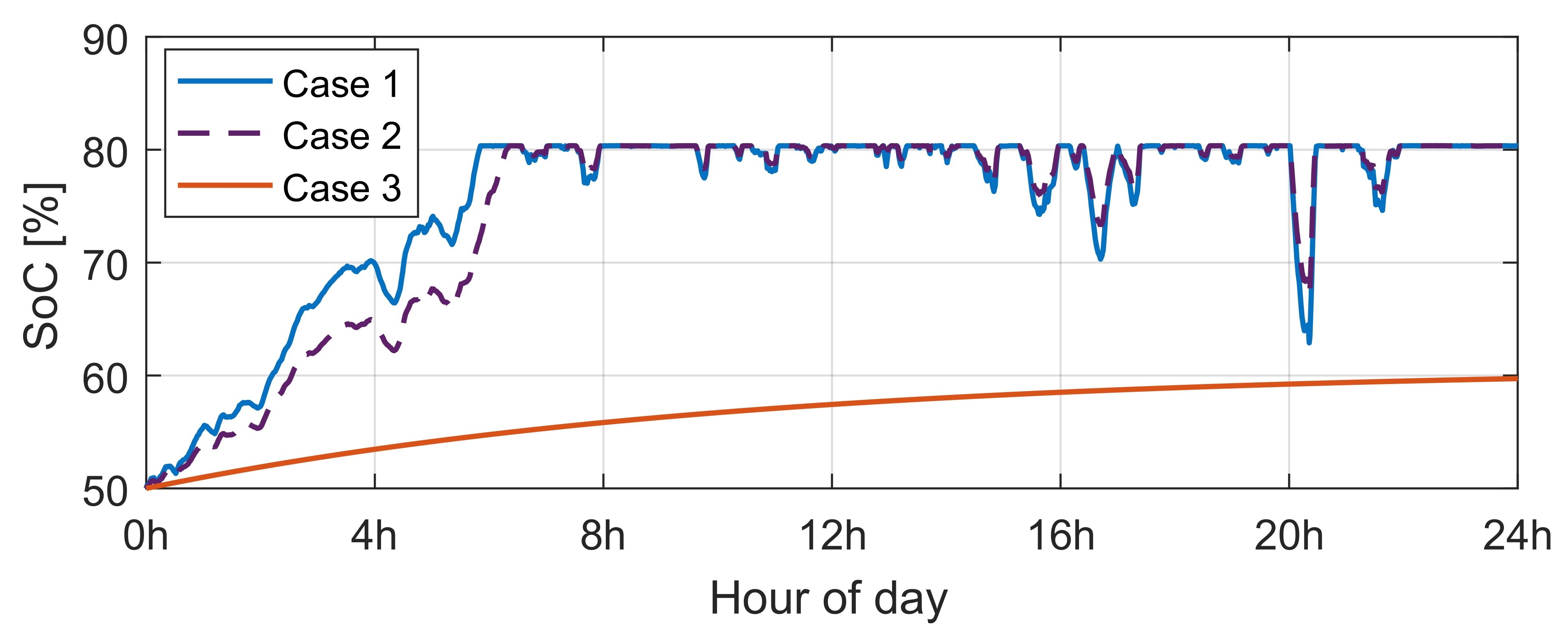
6.1. Scenario 1: Production Is Greater Than Expected

This scenario investigates the HPP’s operating on the island grid when the production is high enough to predominantly require the storage system to be charged. The assumption here was to consider a commitment with a maximum error of $-30\%$ with respect to the average of production. The initial $SoC$ is $50\%$, while $So{C}_{ref}$ is set at $60\%$.

In Scenario 1, three cases are considered: in case 1 more importance is given to the objective relating to $P_{INJ}$, i.e., the interest is focused on the respect of the injection reference. This first case promotes the best profit maximization strategy, by optimizing the amount of power transferred to the storage system that allows holding the injection commitment, in order to avoid penalties and to inject production that will not be billed.

Case 2 considers the same importance given to weight of the objective relating to $P_{INJ}$ (${\lambda }_1$) and the weight of the $SoC$-related objective (${\lambda }_2$). Finally, within case 3, the greater weight was attributed to minimizing the $SoC$ tracking error. Figure 24 presents the power injected by the HPP into the Guadeloupe’s electricity grid over a day, considering the cases 1, 2 & 3. As can be seen in Figure 25 with a higher ${\lambda }_1$ value (case 1), $P_{INJ}$ closely follows the reference $P_{SCHED}$. In case 2, when both objectives have the same weight, the performances are very close to those obtained in case 1. Consequently, the tracking error of the injection set-point is greater in the case 3, and the storage system’s usage is smaller.

Figure 26 shows the $SoC$ levels obtained during test scenario 1. As shown, production curtailments occur when the wind turbines output is above the upper limit of the tolerated injection region, and the BESS is at $80\%$$SoC$. Thus, whereas, in case 1, the curtailment amounts to $0.34\%$, in case 3, this quantity is $0\%$.

As can be appreciated in

Table 4. Key Performance Indicators (KPIs) evaluation for Strategy 1.

Case	CF (%)	${\mathit{P}}_{\mathbf{not}\mathbf{billed}}(\%)$	${\mathit{P}}_{\mathbf{curt}}(\%)$	${\mathit{E}}_{\mathbf{INJ}}$ (MWh)	${\mathbf{BESS}}_{\mathbf{cycles}}$	${\mathit{P}}_{\mathbf{INJ}\mathbf{error}}(\%)$
Case 1	0	0	0.34	56.2	1.90	16.84
Case 2	0	0	0.34	56.2	1.46	18.55
Case 3	8.33	12.16	0	49.9	0.08	28.60

and Figure 26, in case 1 and case 2, there are no commitment failures, and the total amount of energy injected is higher. However, when the BESS is fully charged ($SoC=80\%$), curtailments are present. This is due to fact that the production is greater than the upper band limit, and it is not possible to store more energy. At the same time, the smallest energy injection error was observed, which is coherent with having energy available in the storage system to maintain the injection close to the commitment, unlike case 3, where the BESS is less in demand, and, consequently, the storage system’s lifetime is preserved. We can observe that with a greater ${\lambda }_2$ the storage system remains close to the set-point $So{C}_{ref}$, but the energy injection is smaller.

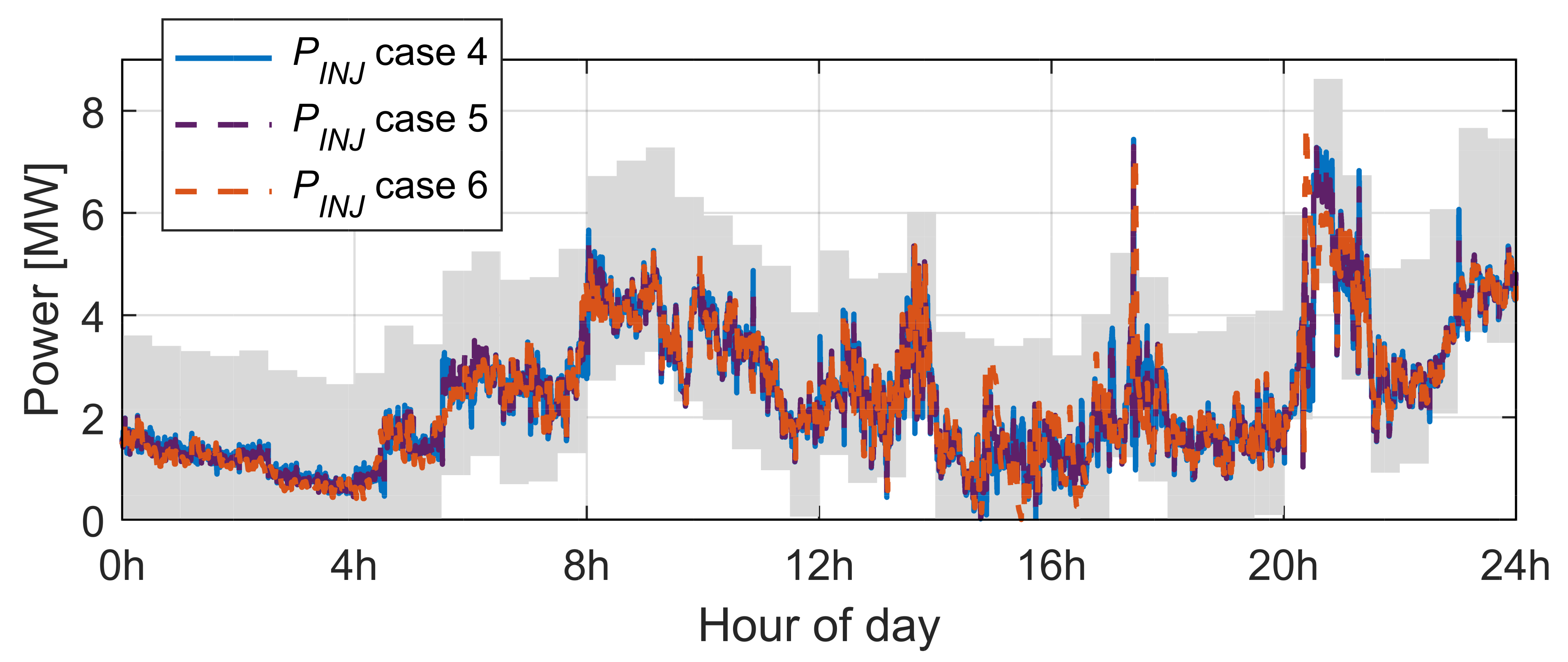
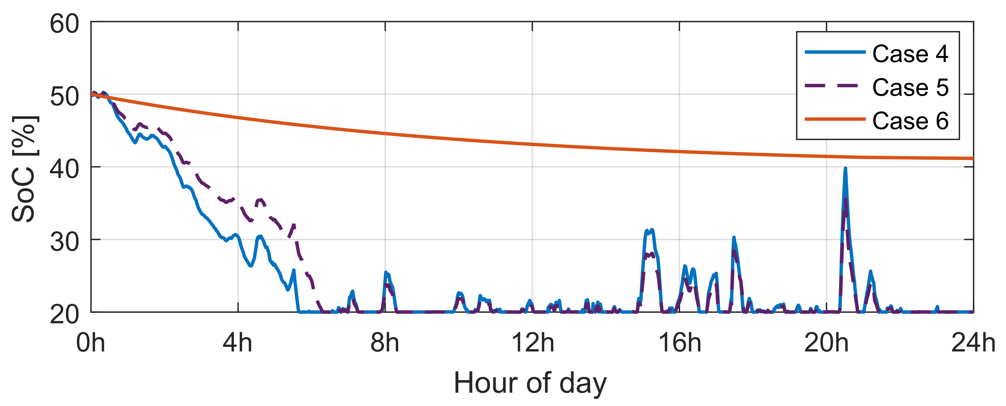
6.2. Scenario 2: Production Lower Than Commitment

Scenario 2 investigates the EMS performance during a period where the production is less than expected. The initial conditions and assumptions considered here are: a maximum commitment error of $30\%$ with respect to the average of production, an initial $SoC$ of $50\%$, while the $So{C}_{ref}$ was established at $39\%$. With lower production compared to the commitment, the objective of the investigated cases is to fulfill the commitment and avoid economic penalties as far as possible.

As for scenario 1 explained above, this scenario presents three cases that are considered with different weights assigned to the objectives:

• case 4, where the greatest weight was assigned to the $SoC$-related objective (${\lambda }_2$) to prioritize minimizing the power injection’s tracking error,
• case 5, the same importance is given to the weight of both objectives, and
• case 6, the greatest weight was attributed to the minimizing the $SoC$ tracking error.

In order to compare with Scenario 1, Figure 27 and Figure 28 present the power injected by the HPP into the Guadeloupe’s electricity grid over a day, while Figure 29 shows the $SoC$ levels obtained during test scenario 2 considering different sets of values for the weights ${\lambda }_1$ and ${\lambda }_2$.

As was observed in previous scenario, Figure 28, with a higher value of ${\lambda }_1$, $P_{INJ}$ follows the BESS reference $P_{SCHED}$ best. Instead, the tracking error of the injection set-point is greater in case 6, considering ${\lambda }_2=100$, and, consequently, the storage system’s usage is smaller.

As can be seen in Figure 29 and in

Table 5. KPIs evaluation for Strategy 2.

Case	CF (%)	${\mathit{P}}_{\mathbf{not}\mathbf{billed}}(\%)$	${\mathit{P}}_{\mathbf{curt}}(\%)$	${\mathit{E}}_{\mathbf{INJ}}$ (MWh)	${\mathbf{BESS}}_{\mathbf{cycles}}$	${\mathit{P}}_{\mathbf{INJ}\mathbf{error}}(\%)$
Case 4	6.25	8.49	0	52.7	2.21	11.70
Case 5	6.25	8.71	0	52.6	1.72	12.91
Case 6	7.64	11.93	0	50.4	0.07	21.47

, in case 4 and case 5, more BESS usage ($BES{S}_{cycles}$) is required to keep to the injection schedule owing to the production which is lower than the commitment. Therefore, the EMS optimizes the injection while allowing smaller variations in the state-of-charge. In case 4 and case 5, a greater power injection is achieved by using the BESS to try to fulfill the commitment. Due to lower production, several times the storage system’s minimum $SoC$ threshold is reached ($20\%$).

Analyzing case 6, with ${\lambda }_1=0$ and ${\lambda }_1=100$, the BESS usage is limited, but, as expected, the amount of the resulting power injection signal is lower. In this case, more importance is given to weight of the objective relating to minimizing of the SoC tracking error, and the BESS is forced to maintain the $So{C}_{ref}$ set at $39\%$. The storage system is used less, but the commitment tracking goal is not reached; therefore, less power is injected into the grid, which causes $P_{INJerror}$ to be greater.

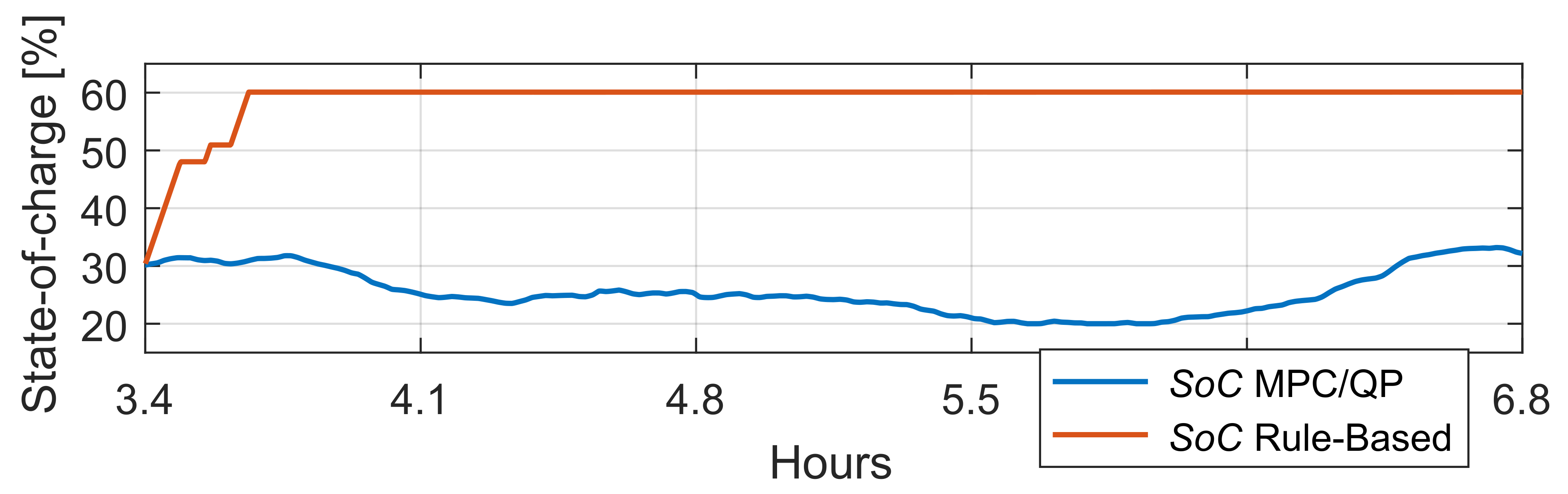
6.3. Comparison with a Rule-Based Strategy

In order to compare the two energy management algorithms, some simulation results are obtained considering a commitment profile with an maximum error of $\pm 10\%$ (shown above in Figure 23). For this simulation both, the MPC/QP and rule-based algorithms in PowerFactory were tested with the following initial conditions: initial $SoC$ of $30\%$ and $So{C}_{ref}=60\%$.

Different values were used for the control objectives weights. Figure 30 plots the resulting BESS power signals for both algorithms. As can be seen, the time of no use of the storage system is longer in the case of the scheme based on rules. In both cases, the more recurrent non-availability of the BESS translates into lesser filtering of the wind turbine production lacks and excesses and, ultimately, the lower injection of power. We can also see that, although the limits of the storage system are the same for both algorithms, the ways in which it is used are very different. While the MPC algorithm used the BESS whenever the $SoC$ is not at its maximum or minimum threshold in order to closely follow the power reference, the rule-based strategy shows an on/off-like behavior with a tendency to use the BESS maximum power either during charging or discharging.

As can be seen in Figure 31, the signal $P_{BESS}$ obtained from the algorithm based on simple rules is zero most of the time. This is because when the $SoC$ is smaller than $So{C}_{ref}=60\%$, and, whenever $P_{WECS}$ is bigger than $P_{SCHED}$, the storage system is charged accordingly to the rules. Moreover, after the $60\%$$SoC$ level is reached, several short time charges take place. On the other hand, the MPC-based controller manages the BESS responding to the instant active power needs (the difference between planned injection and current production).

Figure 32 and Figure 33 plot the state-of-charge charts obtained from the MPC/QP and rule-based algorithms. As can be seen, on several occasions, the MPC/QP algorithm activates the constraints $So{C}^{min}$ and $So{C}^{max}$, i.e., minimum and maximum allowed levels are reached several times. Under the rule-based algorithm, the SoC control evolves between the $40\%$ and $80\%$ levels.

As can be appreciated from Figure 33, the ability of the MPC to both track the reference values and save the lifetime of the BESS leads to an smooth $SoC$ variation during this period. The predictive control-based algorithm varies $P_{BESS}$ to compensate or to absorb power according to the evolution of the instant production, trying to respect the commitment. Meanwhile, the rule-based algorithm limits the use of the storage system due to its simpler operating, which results in BESS being discharged rarely. However, a difference in the final storage levels is observed, which could strongly influence the microgrid management of the following day.

As noted in Figure 34, the tracking of $P_{SCHED}$ is better when using the MPC/QP algorithm. The MPC control strategy is able to optimize the real-time power dispatch and takes into account the preserving the BESS. This is an important factor, especially for stand-alone microgrid configurations.

Table 6. KPIs for comparison of MPC/QP and rule-based algorithms.

	${\mathit{\lambda }}_1=20,{\mathit{\lambda }}_2=80$		${\mathit{\lambda }}_1={\mathit{\lambda }}_2=50$		${\mathit{\lambda }}_1=80,{\mathit{\lambda }}_2=20$
Indicator	MPC	RB	MPC	RB	MPC	RB
$\mathit{CF} (\%)$	1.7	8.5	1.8	8.5	1.7	8.5
${\mathit{P}}_{\mathit{not}\mathit{billed}}(\%$)	0.3	13.6	0.4	13.6	0.4	13.6
${\mathit{P}}_{\mathit{curt}}(\%)$	$5\times {10}^{-4}$	0	$7\times {10}^{-3}$	0	$1\times {10}^{-2}$	0
${\mathit{E}}_{\mathit{INJ}}$ (MWh)	1811.2	1504.5	1807.3	1504.5	1807.5	1504.5
${\mathit{BESS}}_{\mathit{cycles}}$	45.6	15.8	91.2	15.8	111.7	15.8
${\mathit{P}}_{\mathit{INJ}\mathit{error}}(\%)$	0.18	0.24	0.09	0.24	0.06	0.24
${\mathit{SoC}}_{\mathit{error}}(\%)$	20.3	27.7	27.2	27.7	28.7	27.7

summarizes the results obtained from 28-day simulations with three sets of values for ${\lambda }_1$ and ${\lambda }_2$. These results confirm the importance of an optimized algorithm to better manage the energy flow of an HPP when dealing with a day-ahead commitment and demonstrates the effectiveness of the MPC-based strategy proposed.

7. Conclusions

In this paper, an EMS was designed to manage the power dispatch of a hybrid power plant injecting power into the Guadeloupe’s electricity grid. The system combines wind turbines with a Li-ION BESS. The HPP and control structure were modeled using PowerFactory. Moreover, the energy storage system model was validated to be used in the control strategy. Based on this model, the development of an adapted management strategy for predictive control and quadratic programming optimization determined the power flow management of the HPP to comply with the day-ahead commitment according to the WECS output variations. To reach the objectives, a quadratic cost function was formulated that considers the problem’s objectives and is attached to several physical and operational constraints. Using PowerFactory/MATLAB co-simulation, it was proven that the proposed EMS has the ability to handles the battery’s charge/discharge cycles to inject the power into the grid continuously, fulfilling two aims: minimizing the commitment failures and extending the storage system’s lifespan. Several case studies were investigated focusing on the economical or technical aspects of the HPP’s operating. The impact of the tuning parameters was shown through different co-simulation scenarios, allowing the strategy to be adapted over a 28-day period in order to test its performance. It was proven that the proposed strategy based on MPC enables the systematic handling of constraints by managing the optimization problem.

References

1. Chen, F.; Duic, N.; Alves, L.; Carvalho, M. Renewislands—Renewable energy solutions for islands. Renew. Sustain. Energy Rev. 2007, 11, 1888–1902. [Google Scholar] [CrossRef]
2. El-Bidairi, K.S.; Nguyen, H.D.; Jayasinghe, S.; Mahmoud, T.S.; Penesis, I. A hybrid energy management and battery size optimization for standalone microgrids: A case study for Flinders Island, Australia. Energy Convers. Manag. 2018, 175, 192–212. [Google Scholar] [CrossRef]
3. Jin, H.; Liu, P.; Li, Z. Dynamic modeling and design of a hybrid compressed air energy storage and wind turbine system for wind power fluctuation reduction. Comput. Chem. Eng. 2019, 122, 59–65. [Google Scholar] [CrossRef]
4. Moeini-Aghtaie, M.; Dehghanian, P.; Fotuhi-Firuzabad, M.; Abbaspour, A. Multiagent Genetic Algorithm: An Online Probabilistic View on Economic Dispatch of Energy Hubs Constrained by Wind Availability. IEEE Trans. Sustain. Energy 2014, 5, 699–708. [Google Scholar] [CrossRef]
5. Rodrígues, E.; Osório, G.; Godina, R.; Bizuayehu, A.; Lujano-Rojas, J.; Catalão, J. Grid code reinforcements for deeper renewable generation in insular energy systems. Renew. Sustain. Energy Rev. 2016, 53, 163–177. [Google Scholar] [CrossRef]
6. Aidoo, I.; Sharma, P.; Hoff, B. Optimal controllers designs for automatic reactive power control in an isolated wind-diesel hybrid power system. Int. J. Electr. Power Energy Syst. 2016, 81, 387–404. [Google Scholar] [CrossRef]
7. Sosnina, E.; Lipuzhin, I. A Study of Operation Modes of the Autonomous Power Supply System with Wind-Diesel Power Plant. In Proceedings of the 2018 IEEE PES Transmission Distribution Conference and Exhibition—Latin America (T&D-LA), Lima, Peru, 18–21 September 2018; pp. 1–5. [Google Scholar]
8. Aliyu, H.; Agee, J. Electric energy from the hybrid wind-solar thermal power plants. In Proceedings of the 2016 IEEE PES PowerAfrica, Livingstone, Zambia, 28 June–3 July 2016; pp. 264–268. [Google Scholar]
9. Liu, J.; Yao, Q.; Hu, Y. Model predictive control for load frequency of hybrid power system with wind power and thermal power. Energy 2019, 172, 555–565. [Google Scholar] [CrossRef]
10. Wang, Y.; Zhao, M.; Chang, J.; Wang, X.; Tian, Y. Study on the combined operation of a hydro-thermal-wind hybrid power system based on hydro-wind power compensating principles. Energy Convers. Manag. 2019, 194, 94–111. [Google Scholar] [CrossRef]
11. Pathak, G.; Singh, B.; Panigrahi, B. Wind–Hydro Microgrid and Its Control for Rural Energy System. IEEE Trans. Ind. Appl. 2019, 55, 3037–3045. [Google Scholar] [CrossRef]
12. Liu, Y.; Qin, W.; Han, X.; Wang, P. Modelling of large-scale wind/solar hybrid system and influence analysis on power system transient voltage stability. In Proceedings of the 2017 12th IEEE Conference on Industrial Electronics and Applications (ICIEA), Siem Reap, Cambodia, 18–20 June 2017; pp. 477–482. [Google Scholar]
13. Ding, Z.; Hou, H.; Yu, G.; Hu, E.; Duan, L.; Zhao, J. Performance analysis of a wind-solar hybrid power generation system. Energy Convers. Manag. 2019, 181, 223–234. [Google Scholar] [CrossRef]
14. Abdeltawab, H.H.; Mohamed, Y.A.R.I. Market-Oriented Energy Management of a Hybrid Wind-Battery Energy Storage System Via Model Predictive Control With Constraint Optimizer. IEEE Trans. Ind. Electron. 2015, 62, 6658–6670. [Google Scholar] [CrossRef]
15. Hu, J.; Shan, Y.; Xu, Y.; Guerrero, J. A coordinated control of hybrid AC/DC microgrids with PV-wind-battery under variable generation and load conditions. Int. J. Electr. Power Energy Syst. 2019, 104, 583–592. [Google Scholar] [CrossRef] [Green Version]
16. El-Bidairi, K.S.; Nguyen, H.D.; Mahmoud, T.S.; Jayasinghe, S.; Guerrero, J.M. Optimal sizing of Battery Energy Storage Systems for dynamic frequency control in an islanded microgrid: A case study of Flinders Island, Australia. Energy 2020, 195, 117059. [Google Scholar] [CrossRef]
17. Kennedy, N.; Miao, C.; Wu, Q.; Wang, Y.; Ji, J.; Roskilly, T. Optimal Hybrid Power System Using Renewables and Hydrogen for an Isolated Island in the UK. Energy Procedia 2017, 105, 1388–1393. [Google Scholar] [CrossRef]
18. Katsigiannis, Y.; Karapidakis, E. Operation of wind-battery hybrid power stations in autonomous Greek islands. In Proceedings of the 2017 52nd International Universities Power Engineering Conference (UPEC), Heraklion, Greece, 28–31 August 2017; pp. 1–5. [Google Scholar]
19. Obara, S.; Sato, K.; Utsugi, Y. Study on the operation optimization of an isolated island microgrid with renewable energy layout planning. Energy 2018, 161, 1211–1225. [Google Scholar] [CrossRef]
20. Ntomaris, A.; Bakirtzis, A. Stochastic Scheduling of Hybrid Power Stations in Insular Power Systems With High Wind Penetration. IEEE Trans. Power Syst. 2016, 31, 3424–3436. [Google Scholar] [CrossRef]
21. Notton, G.; Mistrushi, D.; Stoyanov, L.; Berberi, P. Operation of a photovoltaic-wind plant with a hydro pumping-storage for electricity peak-shaving in an island context. Sol. Energy 2017, 157, 20–24. [Google Scholar] [CrossRef]
22. Wang, C.; Liu, Y.; Li, X.; Guo, L.; Qiao, L.; Lu, H. Energy management system for stand-alone diesel-wind-biomass microgrid with energy storage system. Energy 2016, 97, 90–104. [Google Scholar] [CrossRef]
23. Luna, A.; Díaz, N.; Graells, M.; Vásquez, J.; Guerrero, J. Mixed-Integer-Linear-Programming-Based Energy Management System for Hybrid PV-Wind-Battery Microgrids: Modeling, Design, and Experimental Verification. IEEE Trans. Power Electron. 2017, 32, 2769–2783. [Google Scholar] [CrossRef] [Green Version]
24. Menniti, D.; Pinnarelli, A.; Sorrentino, N.; Vizza, P.; Burgio, A.; Brusco, G.; Motta, M. A Real-Life Application of an Efficient Energy Management Method for a Local Energy System in Presence of Energy Storage Systems. In Proceedings of the 2018 IEEE International Conference on Environment and Electrical Engineering and 2018 IEEE Industrial and Commercial Power Systems Europe (EEEIC / I CPS Europe), Palermo, Italy, 12–15 June 2018; pp. 1–6. [Google Scholar]
25. Bukar, A.; Tan, C. A review on stand-alone photovoltaic-wind energy system with fuel cell: System optimization and energy management strategy. J. Clean. Prod. 2019, 221, 73–88. [Google Scholar] [CrossRef]
26. Petersen, L.; Iov, F.; Tarnowski, G.C. A Model-Based Design Approach for Stability Assessment, Control Tuning and Verification in Off-Grid Hybrid Power Plants. Energies 2019, 13, 49. [Google Scholar] [CrossRef] [Green Version]
27. Zhang, Y.; Meng, F.; Wang, R.; Kazemtabrizi, B.; Shi, J. Uncertainty-resistant stochastic MPC approach for optimal operation of CHP microgrid. Energy 2019, 179, 1265–1278. [Google Scholar] [CrossRef]
28. Tan, K.T.; Sivaneasan, B.; Peng, X.Y.; So, P.L. Control and Operation of a DC Grid-Based Wind Power Generation System in a Microgrid. IEEE Trans. Energy Convers. 2016, 31, 496–505. [Google Scholar] [CrossRef]
29. Zhang, Y.; Meng, F.; Wang, R.; Zhu, W.; Zeng, X.J. A stochastic MPC based approach to integrated energy management in microgrids. Sustain. Cities Soc. 2018, 41, 349–362. [Google Scholar] [CrossRef]
30. Xing, X.; Xie, L.; Meng, H. Cooperative energy management optimization based on distributed MPC in grid-connected microgrids community. Int. J. Electr. Power Energy Syst. 2019, 107, 186–199. [Google Scholar] [CrossRef]
31. Tedesco, F.; Mariam, L.; Basu, M.; Casavola, A.; Conlon, M.F. Economic Model Predictive Control-Based Strategies for Cost-Effective Supervision of Community Microgrids Considering Battery Lifetime. IEEE J. Emerg. Sel. Top. Power Electron. 2015, 3, 1067–1077. [Google Scholar] [CrossRef]
32. Zhang, X.; Bao, J.; Wang, R.; Zheng, C.; Skyllas-Kazacos, M. Dissipativity based distributed economic model predictive control for residential microgrids with renewable energy generation and battery energy storage. Renew. Energy 2017, 100, 18–34. [Google Scholar] [CrossRef]
33. Chen, Y.; Deng, C.; Li, D.; Chen, M. Quantifying cumulative effects of stochastic forecast errors of renewable energy generation on energy storage SOC and application of Hybrid-MPC approach to microgrid. Int. J. Electr. Power Energy Syst. 2020, 117, 105710. [Google Scholar] [CrossRef]
34. Tabar, V.S.; Abbasi, V. Energy management in microgrid with considering high penetration of renewable resources and surplus power generation problem. Energy 2019, 189, 116264. [Google Scholar] [CrossRef]
35. Notton, G. Importance of islands in renewable energy production and storage: The situation of the French islands. Renew. Sustain. Energy Rev. 2015, 47, 260–269. [Google Scholar] [CrossRef]
36. Belfort, A. Les Chiffres Clés de l’Énergie en Guadeloupe, 2016 ed.; Technical report; Observatoire régional de l’énergie et du climat de la Guadeloupe; Comité de l’OREC (ADEME, Région Guadeloupe, DEAL, EDF, Météo-France, SYMEG et Synergîle): Baie-Mahault, France, 2017. [Google Scholar]
37. Marin, D. Intégration des éoliennes dans les réseaux électriques insulaires. Ph.D. Thesis, Ecole Centrale de Lille, Lille, France, 2009. [Google Scholar]
38. Aguilera-González, A.; Vechiu, I.; Rodríguez, R.H.L.; Bacha, S. MPC Energy Management System For A Grid-Connected Renewable Energy/Battery Hybrid Power Plant. In Proceedings of the 7th International Conference on Renewable Energy Research and Applications (ICRERA 2018), Paris, France, 14–17 October 2018; pp. 738–743. [Google Scholar]
39. Rueda, J.; Korai, A.; Cepeda, J.; Erlich, I.; Gonzalez-Longatt, F. Implementation of Simplified Models of DFIG-Based Wind Turbines for RMS-Type Simulation in DIgSILENT PowerFactory. In PowerFactory Applications for Power System Analysis; Springer International Publishing: Cham, Switzerland, 2014. [Google Scholar]
40. Yazhou, L.; Mullane, A.; Lightbody, G.; Yacamini, R. Modeling of the wind turbine with a doubly fed induction generator for grid integration studies. IEEE Trans. Energy Convers. 2006, 21, 257–264. [Google Scholar]
41. Tremblay, O.; Dessaint, L. Experimental validation of a battery dynamic model for EV applications. World Electr. Veh. J. 2009, 3, 289–298. [Google Scholar] [CrossRef] [Green Version]
42. Saw, L.; Somasundaram, K.; Ye, Y.; Tay, A. Electro-thermal analysis of Lithium Iron Phosphate battery for electric vehicles. J. Power Sources 2014, 249, 231–238. [Google Scholar] [CrossRef]
43. Rigo-Mariani, R. Méthodes de Conception Intégrée “Dimensionnement-Gestion” par Optimisation d’Un Micro-réseau avec Stockage. Ph.D. Thesis, Université de Toulouse, Toulouse, France, 2015. [Google Scholar]
44. Hérnandez-Torres, D.; Turpin, C.; Roboam, X.; Sareni, B. Modélisation en flux d’énergie d’une batterie Li-Ion en vue d’une optimisation technico-économique d’un micro-réseau intelligent. In Proceedings of the Symposium de Génie Electrique (SGE’16), Grenoble, France, 7–9 March 2016; pp. 1–8. [Google Scholar]
45. Camacho, E.; Bordons-Alba, C. Model Predictive Control; Springer Verlag: London, UK, 2007. [Google Scholar]
46. Efheij, H.; Albagul, A.; Ammar Albraiki, N. Comparison of Model Predictive Control and PID Controller in Real Time Process Control System. In Proceedings of the 2019 19th International Conference on Sciences and Techniques of Automatic Control and Computer Engineering (STA), Sousse, Tunisia, 24–26 March 2019; pp. 64–69. [Google Scholar]
47. Alamir, M. A Pragmatic Story of Model Predictive Control: Self-Contained Algorithms and Case-Studies; CreateSpace Independent Publishing Platform: Grenoble, France, 2013. [Google Scholar]
48. Coleman, T.; Li, Y. A Reflective Newton Method for Minimizing a Quadratic Function Subject to Bounds on Some of the Variables. SIAM J. Optim. 1996, 6, 1040–1058. [Google Scholar] [CrossRef]
49. Pramangioulis, D.; Atsonios, K.; Nikolopoulos, N.; Rakopoulos, D.; Grammelis, P.; Kakaras, E. A Methodology for Determination and Definition of Key Performance Indicators for Smart Grids Development in Island Energy Systems. Energies 2019, 12, 242. [Google Scholar] [CrossRef] [Green Version]
50. Gundogdu, B.; Gladwin, D.T. A Fast Battery Cycle Counting Method for Grid-Tied Battery Energy Storage System Subjected to Microcycles. In Proceedings of the 2018 International Electrical Engineering Congress (iEECON), Krabi, Thailand, 7–9 March 2018; pp. 1–4. [Google Scholar]
Figure 1. Available power in Guadeloupe’s power grid by type of primary energy in 2018.
Energies 14 01066 g001
Figure 2. Guadeloupe’s PowerFactory electric grid model.
Energies 14 01066 g002
Figure 3. Hybrid power plant diagram: wind farm and battery storage.
Energies 14 01066 g003
Figure 4. Sainte-Rose substation in Guadeloupe electrical grid.
Energies 14 01066 g004
Figure 5. Wind generation system modeled via PowerFactory.
Energies 14 01066 g005
Figure 6. Doubly Fed Induction Generators (DFIG) wind turbine’s characteristic curve.
Energies 14 01066 g006
Figure 7. Battery discharge curves: red line, SimPowerSystems battery, and implemented nonlinear Treblay model in gray.
Energies 14 01066 g007
Figure 8. Discharge battery model.
Energies 14 01066 g008
Figure 9. Validation of MATLAB implementation: (a) input current. In (bd) the signals obtained for i t , i * and S o C are compared.
Energies 14 01066 g009
Figure 10. Percentage errors of: (a) i t , (bc) comparison of i * and S o C signals obtained.
Energies 14 01066 g010
Figure 11. Intensium Max 20M (IM20M) storage system discharge curve, (a) power discharge and (b) state-of-charge.
Energies 14 01066 g011
Figure 12. Battery Energy Storage System (BESS) model validation: (a) power reference profile and active power obtained, (b) battery current, (c) S o C , (d) i t .
Energies 14 01066 g012
Figure 13. Battery energy storage system modeled via PowerFactory.
Energies 14 01066 g013
Figure 14. System inputs and outputs.
Energies 14 01066 g014
Figure 15. Hybrid power plant (HPP) modeling: inputs and outputs. (a) Integral current i t , (b) Filtered current i * , (c) SOC and (d) BESS active power.
Energies 14 01066 g015
Figure 16. BESS model control diagram.
Energies 14 01066 g016
Figure 17. HPP power injection band.
Energies 14 01066 g017
Figure 18. Model predictive control with quadratic programming (MPC/QP) strategy structure.
Energies 14 01066 g018
Figure 19. The power injection set-point.
Energies 14 01066 g019
Figure 20. Simple rule-based management algorithm.
Energies 14 01066 g020
Figure 21. PowerFactory/MATLAB co-simulation scheme.
Energies 14 01066 g021
Figure 23. Commitment profiles, 28-day period.
Energies 14 01066 g023
Figure 24. Scenario 1: Injected power and tolerated band/injection region.
Energies 14 01066 g024
Figure 25. Scenario 1: Zoom in the njected power and tolerated band/injection region.
Energies 14 01066 g025
Figure 26. Scenario 1: state-of-charge ( S o C ) signals with Case 1: λ 1 = 100 , λ 2 = 0 , Case 2: λ 1 = λ 2 = 50 , and Case 3: λ 1 = 0 , λ 2 = 100 . Initial SoC: 50 % and P S C H E D with maximum ± 30 % error.
Energies 14 01066 g026
Figure 27. Scenario 2: Injected power and tolerated band/injection region.
Energies 14 01066 g027
Figure 28. Zoom Scenario 2: Injected power and tolerated band/injection region.
Energies 14 01066 g028
Figure 29. Strategy 2: S o C signals with Case 4: λ 1 = 100 , λ 2 = 0 , Case 5: λ 1 = λ 2 = 50 , and Case 6: λ 1 = 0 , λ 2 = 100 . Initial SoC of 50 % and P S C H E D with maximum ± 30 % error.
Energies 14 01066 g029
Figure 30. MPC/QP and rule-based algorithms: storage system power with λ 1 = λ 2 = 50 , commitment with maximum 10 % error, initial S o C of 50 % , and 50 % as S o C set-point.
Energies 14 01066 g030
Figure 31. Close view of BESS power using MPC/QP and rule-based algorithms in PowerFactory.
Energies 14 01066 g031
Figure 32. MPC/QP and rule-based algorithms: state-of-charge with λ 1 = λ 2 = 50 , commitment with maximum 10 % error, initial S o C of 50 % , and 50 % as S o C set-point.
Energies 14 01066 g032
Figure 33. Close view of state-of-charge using MPC/QP and rule-based algorithms in PowerFactory.
Energies 14 01066 g033
Figure 34. Zoom in the total power injected by the HPP into the Guadeloupe island electric grid using MPC/QP and rule-based algorithms in PowerFactory.
Energies 14 01066 g034