Abstract
Large-scale offshore wind farms (OWF) are under construction along the southeastern coast of China, an area with a high typhoon incidence. Measured data and typhoon simulation model are used to improve the reliability of extreme wind speed (EWS) forecasts for OWF affected by typhoons in this paper. Firstly, a 70-year historical typhoon record database is statistically analyzed to fit the typhoon parameters probability distribution functions, which is used to sample key parameters when employing Monte Carlo Simulation (MCS). The sampled typhoon parameters are put into the Yan Meng (YM) wind field to generate massive virtual typhoon in the MCS. Secondly, when typhoon simulation carried out, the change in wind field roughness caused by the wind-wave coupling is studied. A simplified calculation method for realizing this phenomenon is applied by exchanging roughness length in the parametric wind field and wave model. Finally, the extreme value theory is adopted to analyze the simulated typhoon wind data, and results are verified using measured data and relevant standards codes. The EWS with 50-year recurrence of six representative OWF is predicted as application examples. The results show that the offshore EWS is generally stronger than onshore; the reason is sea surface roughness will not keep growing accordingly as the wind speed increases. The traditional prediction method does not consider this phenomenon, causing it to overestimate the sea surface roughness, and as a result, underestimate the EWS for OWF affected by typhoons. This paper’s methods make the prediction of EWS for OWF more precise, and results suggest the planer should choose stronger wind turbine in typhoon prone areas.
1. Introduction
According to the 13th Five-Year Plan for Wind Power Development, China will vigorously develop offshore wind power. By 2020, the scale of OWF construction will reach 10 GW, and the cumulative grid-connected capacity will reach over 5 GW. However, an essential factor restricting OWF development in China and North America is that these regions are in high-prone areas of tropical cyclones (also called typhoons in China, hereinafter referred to as typhoons). There were 652 typhoons landed in China between 1949 and 2003, the landfall typhoons that may cause significant damage to wind farms to account for 29.4%, and there is an average of 3.49 per year [1]. Typhoon Dujuan in September 2003, Typhoon Sangmei in 2006, Typhoon Tiantu in 2013, and Super Typhoon Rammasun in 2014 all caused severe damage to wind farms along the coast of China. Typhoon Maemi landed on Miyakojima, Japan, in 2003, caused significant damage to Japanese onshore wind farms [2]. In 2015, Typhoon Soudelor hit Taiwan Taichung, resulted in five wind turbines’ damage. Worsnop et al. [3] pointed out that when a typhoon passes through a wind farm, especially in extreme cases, the typhoon eyewall passes by, both the average EWS and turbulence intensity will exceed the values specified by the current standards code through observational data and simulations. The occurrence of these wind farm accidents and the analysis of scholars show the necessity for further exploring the prediction of EWS for OWF under typhoons’ influence.
The typical method for predicting EWS is analyzing the historical meteorological record data and then calculating it with a specific recurrence period by employing the extreme value theory. Guglielmo et al. [4] collected meteorological observation data to study extreme wind speed distribution through the improved generalized Pareto distribution, compared with the fitting results of Weibull distribution, studied the EWS of wind farm under the hurricane’s influence. However, due to the limited meteorological observation stations set along with China coastal areas, the meteorological observation data that have been recorded are incomplete. Therefore, the above method based on historical meteorological records is not feasible for predicting the EWS of OWF during the whole life cycle in China. According to the latest version of IEC standard 61400-1, fourth edition released by International Electrotechnical Organization (IEC) in 2019 [5], as well as Chinese national standard GB/T 31519 [6], applying MCS is appropriate for predicting the EWS of OWF in typhoon prone areas of northwest pacific. The specific method simulates massive typhoons and establishes the probability distribution model of annual maximum extreme wind speeds caused by each typhoon and then deduce the EWS of each recurrence period. Ishihara et al. [7] proved that the EWS uncertainty of the MCS result is smaller than that by Gumbel method through adopting a simplified wind field model and Computational Fluid Dynamics to MCS and analyzing short-term observation data of Japan OWF. In the field of building load, many scholars, such as Zhao et al. [8], Xiao et al. [9], and Wang et al. [10], have been working on the EWS, wind pressure, and vulnerability of China’s coastal high-rise buildings based on MCS and parametric typhoon wind field models.
As mentioned above, the MCS has been generally accepted as a wind speed prediction method. The critical issue of adopting the MCS to predict EWS is how to simulate typhoons based on limited observation data and generate enough credible wind speed samples. Generally, typhoon simulation models can be classified into meteorological models and parametric typhoon field models [11]. High-resolution dynamic models (Meteorological models) are, at present, too computationally expensive to be applied directly to risk assessment, which should involve very large numbers of simulations to cover nearly all possible scenarios. Consequently, much more computationally efficient parametric models are often used in risk analysis. Parametric wind and pressure models can also be applied to storm surge analysis. Such parametric modelling and analysis can be readily coupled with TC risk models to estimate TC hazard risk [12]. For example, it costs three days for the 34-day Fiji island simulations when performing WRF on the New Zealand Science Infrastructure (NeSI) High-Performance Computer—Mahuika [13]. The computational costs of parametric and meteorological models differ by orders of magnitude. The use of numerical wave models, forced with parametric wind fields, is a common practice within the climatic characterization of extreme events [14].
Parametrical models maybe classified into two categories: Numerical models and analytical models. Numerical models have often been developed by simplifying the three-dimensional Navier–Stokes equations through introduction of some empirical formulas based on the observation data of typhoons in the field. The solutions are then sought by using numerical methods [15], such as the Vickery model [16]. Analytical models such as [17,18,19] use perturbation analysis to obtain the tangential boundary layer velocity in the friction region. The parameters input for the simplified wind field models greatly influence the results, especially terrain condition of the target site affects the EWS and turbulence intensity of simulated wind [20]. Previous studies focused on the onshore conditions, where the terrain state is relatively easy to obtain. The terrain state z0 has been explicitly defined by provisions documented for building load specifications and other relevant specifications. It can still be obtained by carrying out wind tunnel experiments even for complex geomorphic features.
When the wind blows across the sea, it will cause seawater to move violently, namely wind-induced waves. Simultaneously, the wave fluctuation will hinder the airflow on its surface, forming the sea surface’s wind-wave coupling phenomenon. This phenomenon is more important in case of typhoon or other storm events. To take the wind-wave coupling into account, the mainstream approach is to take the factor that waves affecting roughness length z0 or resistance coefficient Cd [20]. The calculation of sea surface roughness can be divided into two categories: Parameter fitting method and momentum conservation equation-based derivation method. The parameter fitting method is widely used in engineering. It mainly uses the measured values of wind state or wave parameters to fit the surface roughness parameter z0 or ground resistance parameter Cd. Charnock formula is the basement of parametric dynamic roughness algorithm, which have been used by IEC standard [21]. The Fairall form [22] is the default approach for z0 in the Weather and Research Model (WRF) model. Taylor et al. [23], Zijlema et al. [24], Edson et al. [25], used observed values from different stations to fit the parameter of the Charnock formula and put forward improvement. Many researchers have tried to introduce the wave impact on the Charnock parameter in terms of derived wave parameters. For instance, the Fan [26] scheme adds a dependence upon wave age Cp/u∗, and Liu et al. [27] further include a u∗-based correction factor for the effect of spray along with Cp/u∗. Another method, the theoretical momentum conservation equation-based derivation approach of calculating z0 and Cd is through the momentum conservation within the wave boundary layer. Janssen First proposed this method [28], and Janssen et al. [29], Chalikov et al. [30], and Makin et al. [31], further improved this method. Janssen [28] successfully developed a wind-wave coupling approach that has been widely applied in many ocean-wave models.
Drost et al. [32] employed the parametric wind field model to drive the SWAN (Simulating Waves Nearshore) model to simulate waves caused by wind when a typhoon passed through. The accuracy of the model was verified by the measurement from buoys and weather stations. The measurement and simulation results prove that typhoon provides continuous energy to sea waves and promotes sea waves development. Guo et al. [33] collected observation data statistics in Shenzhen, the southeast coastal city under the influence of typhoon. They analyzed the wind distribution characteristics, with YM wind field model simulating cyclone and SWAN plus Advanced Circulation (SWAN + ADCIRC) coupled model simulating the extreme wave height during the storm surge, then analyzed the risk of intense waves. Still, Guo did not consider the influence of sea surface roughness on EWS. Yan et al. [34]. used a parametric wind field model to study the distribution of EWS of ultra-long recurrence period in the south China sea, and the EWS distribution for different sites through the simulating stochastic process. Still, they ignored the influence of roughness on wind field simulation, either. Larsen et al. [20] coupled the atmospheric Weather Research and Forecasting (WRF) model and SWAN model through a wave boundary layer model (WBLM) that is implemented in SWAN. They exchanged the sea surface roughness length between the two models to realize the air–wave coupling. They studied the wind speed distribution of the offshore wind field affected by sea waves and then predicted the EWS. The results showed that implementing the coupling method can get a more precise prediction value. However, Larsen’s process is computationally expensive and cannot be applied in the MCS. Therefore, how to deal with the wind-wave coupling effect when predicting EWS with a specific recurrence period still needs further study.
To further improve the accuracy of EWS prediction affected by typhoons for OWF along the southeast coast of China, six representative OWF being planned or under construction are selected as the performance objects. The 70-year typhoon record data from the China central meteorological station is used to statistical analysis. The critical parameters of those typhoons that affect the six OWF are fitted by probability distribution function. When taking out MCS, Metropolis–Hastings algorithm is applied to sample the key parameters of synthesis typhoon. The probability distribution function fitted is used as the target function in the Metropolis-Hastings algorithm. Then, the key parameters will be input into the YM typhoon field model to generate enough simulated typhoons. By repeating the above process large number of times, we can get massive synthesis typhoon speed data. Finally, the EWS with certain recurrence period is got by adopted the massive synthesis typhoon speed data to extreme value analysis. Moreover, to investigate the influence of wind-wave coupling on the simulation results, exchanged parameters are set up, the impact of sea waves on atmospheric boundary layer roughness length is introduced into YM wind field model, and a simplified relationship between wind speed and roughness length is also proposed. Finally, the simulation results are compared with the measured data to verify the accuracy of the model. A summarization of the influence of the wind-wave coupling model on the prediction of EWS of OWF is made. The EWS of the six aforementioned OWF has been predicted through the propose modified model.
2. Theory and Method
2.1. MCS and Process
The MCS was proposed as a fundamental numerical calculation method guided by probability and statistics theory in the mid-1940s, with the rapid development of science and technology, accompanying the electronic computer’s invention, is widely used in financial engineering, macroeconomics, computational physics, and other fields [35]. The key to applying the MCS to predict EWS caused by typhoons is transforming the process into a probability and statistics problem. That is, generating massive synthetic typhoons through computer simulation, statistically analyzing the wind of simulated typhoon affected the target point, and employing the extreme value theory to fit the statistical data for EWS with a specific recurrence period, as is shown in Figure 1. The key parameters characterizing a typhoon include central pressure difference ∇p, moving speed c, typhoon path direction β, the minimum distance dmin between simulation point and typhoon track, and maximum wind radius rmax. To facilitate the MCS, the concept of simulation circle is usually adopted. That is, the target site is selected as the center of the circle, and typhoon track within the circle will be selected as the research object, where the radius of a circle R = 500 km is selected in this paper. The specific steps of predicting EWS for an OWF in the MCS are as follows:
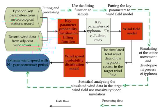
Figure 1.
Flow chart of extreme wind speed (EWS) forecasts for offshore wind farms (OWF) by Monte Carlo method.
- Collect typhoon key parameters record from meteorological stations and adjacent wind tower’s wind speed historical records.
- Fit and statistical process the data to get the key parameter probability distribution fitting function.
- Use the fitting function and Metropolis–Hastings algorithm (‘mhsample‘ function of Matlab software is applied in this paper [36]) to sample key typhoon parameters.
- Put the key typhoon parameters to YM wind model to simulate the entire movement and development process of typhoon and get the total wind data of the typhoon course.
- Repeat step 3–4 for 106 (or more) times to get massive wind data.
- Statistical analyze the massive wind data and get wind speed probability distribution model.
- Use probability distribution model (generalized extreme value theory in this paper) to get the EWS with a certain return period.
2.2. YM Typhoon Wind Field Model
YM typhoon model is a parametric model, which, based on the momentum equation of atmospheric motion, establishes the horizontal momentum equation in the atmospheric gradient layer and boundary layer [19]:
where is the air density, f is the Coriolis coefficient, k is the unit vector normal of the axis of rotation of the earth, F is the boundary layer friction, the typhoon-induced wind velocity v is expressed by the addition of the gradient wind vg in the free atmosphere, and the component v′, caused by the friction on the ground surface, in the boundary layer, when v′ was brought into Equation (1), and disregarded as (in the typhoon boundary layer) [19], the formula can be changed into:
The perturbation method can be adopted to solve the Equation (2), and the boundary layer condition is introduced:
Here, z and z’ denote different vertical coordinate axes. For detailed definitions, see Yang Meng’s paper [19]. vs is the friction velocity at the lower boundary of the wind field, and z = 0 denotes the ground surface. If wind speed profile near the surface conforms with logarithmic law, then the relationship between the resistance coefficient Cd and the surface roughness length z0 can be expressed as follows:
where κ is the Karman constant, take κ = 0.4; the average surface roughness element height h can be calculated by h = Az00.86 [37], where the constant A is usually taken as 11.4 [38,39]; d is the zero plane displacement, which is calculated by d = 0.75h [40].
2.3. Generalized Extreme Value Theory
The generalized extreme value theory can be used to fit the annual extreme wind speed of wind farms under mixed climate conditions affected by extreme weather conditions such as hurricanes or typhoons [4]. Gumbel distribution is commonly selected by national steel structure associations of China, Canada, the United States, etc. It is applied to fit the typhoon’s annual EWS in this paper.
The relationship between guarantee probability P and recurrence T (unit year) is:
The design maximum wind speed with corresponding recurrence period T is:
where μT, αT is the parameter to be fitted.
2.4. Offshore Roughness Calculation Considering the Wind-Wave Coupling Effect
The distribution of horizontal wind speed along the vertical direction of the wind field can be described by logarithmic rate, and the wind speed at height z is calculated via:
where z denotes equivalent ground roughness length, the simulated points can be obtained by consulting the relevant standards when they are located on the land, and the wind tunnel is necessary for determining the special conditions. However, when simulating EWS for offshore, the effect of wind-wave coupling needs to be considered, and the influence of wave on roughness along with consequent influence on drag coefficient should be introduced.
To solve wind-wave coupling, the mainstream approach taking the factor that waves affecting roughness length z0 and using it as the exchange parameter between meteorological and wave fluid models [20]. In order to describe the change of roughness caused by sea waves, Charnock et al. [21] proposed the dynamic parameterization scheme of sea surface roughness: , among which is the empirical constant 0.011, is the friction velocity, is the gravitational acceleration constant. Fairall et al. [22] adds a smooth current term on the sea surface based on Charnock’s model, which is further improved to , v is the kinematic viscosity of seawater (at 20 ℃). Taylor et al. [23] further distinguished the scheme with different wind speeds: , where:
In order to simplify the relationship, the empirical relationship given by Wu et al. [41], where is the resistance coefficient at the height of 10 m, and is the wind speed at the height of 10 m, then through the formula , induces , and take into the Equation (9) and get:
IEC standard (IEC 61400-4) suggested that the relationship between dynamic sea surface roughness z0 and wind speed at hub is [42]:
In the Equation (12), denotes Charnock constant, for open sea condition, while for offshore condition, .
3. Result and Discussion
3.1. Parameters Setting and Verification of Parametric Wind Field Model
In order to verify the applicability of the YM typhoon wind field model and the rationality of the critical parameters used in this paper, the model is adopted to simulate the NO.1911 typhoon “Bailu” in 2019 and obtain the wind speed on the coastal islands of eastern Guangdong, and which is compared with the measured result received from experimental observation station of Shantou University. The observation station is located on Nan’ao island of Shantou City, covering an area of more than 2 hectares. The observation station’s latitude and longitude are 23.481° N, 117.110° E. The wind tower at the station is less than 100 m away from the coastline, back to a gentle slope hill, and it faces to a beach, which causes the roughness length of different wind directions to be different. In this paper, roughness length is changed in the range of 0.001~0.12 m. The altitude of the installation point of the anemometer is 12 m, and the installation height of the anemometer is 10 m from the ground. The parameter information for YM model in this manuscript is obtained from the typhoon network of the China central meteorological station [43]. The typhoon track and relative position with the observation station is shown in Figure 2. Since the meteorological observation data do not contain the radial pressure distribution, the Holland pressure profile is used to describe the pressure distribution of typhoon field [44]. The typhoon pressure profile parameter B is determined by the Equation (13), which is got by reverse calculating the data from the observation station, and the maximum wind speed radius rmax is determined by the scheme defined by Equation (14) fitted by reference [45]. The observed wind speed from the station during the typhoon passed by was selected to compare with the data from the YM typhoon model, as is shown in Figure 3. It can be seen from the figure that the model and critical parameters settings in this manuscript can effectively simulate the whole process of a typhoon in the southeast coastal area.
where p(r) is the pressure value at the distance r from the typhoon center in polar coordinates, p0 is central pressure is the central pressure, ∇p is the difference between the ambient pressure p∞ and the central pressure p0.
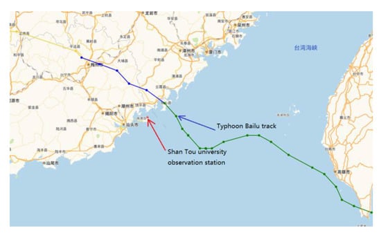
Figure 2.
Typhoon Bailu track and its relative position with observation station.
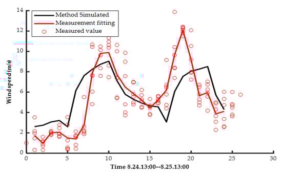
Figure 3.
Comparison of measured and simulated wind speed at observation stations during Typhoon Bailu.
3.2. Statistics and Fitting of Critical Parameters of Typhoons
To study the EWS distribution of OWF affected by typhoons, the CMA tropical cyclone best-path dataset, which records the location and intensity data of tropical cyclones every 6 h, is introduced (the data are available on reference [43]). It was searched from north of the equator and west of 180° E, and the area covering the South China Sea, from 1949 to 2018 [46], is chosen for typhoon statistical analysis. When a typhoon track within the radius of 500 km, it was chosen for analysis. The key parameters of typhoon include the annual probability of occurrence λ, moving direction β (zero eastward, positive counterclockwise rotation), central pressure difference ∇p, moving speed c, and minimum distance dmin. The above parameters are usually fitted with specific probability distribution functions, which will be regarded as the target function when using the Metropolis-Hastings algorithm to sample virtual typhoon parameters in MCS. The critical parameters fitting result of six representative OWF of Guangdong province 13th Five-Year plan is shown in Table 1. The parameters distribution of the representative wind farm Yang Dong in Shantou ocean near Shantou university observation station is shown in Figure 4 below. There are differences between typhoon critical parameters distribution for different station. However, although the overall distribution still conforms to the distribution function given in Table 1, the parameters of the distribution function are different. The specific parameters of the fitting function for six wind farms are shown in Table 2.

Table 1.
Function fitting of typhoon key parameters distribution.
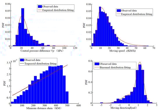
Figure 4.
Fitting results of key parameters of typhoon in the wind farm of Shantou Yang Dong OWF.
Table 2.
Parameters of fitting function for typhoon key parameters of six representative OWF in Guangdong Province.
3.3. Prediction of EWS under the Influence of Typhoon without the Parametrization of Surface Roughness
When applying the YM in this paper, without considering wind–wave coupling, the sea surface roughness length over sea can be assumed z0 = 0.001 m [47]. The EWS and wind direction of Yangdong under the influence of typhoon is predicted. The results are shown in Figure 5a. The 1-h averaged wind speed in each direction with a 50-year recurrence period at the hub height (100 m) is 42.82 m/s. The converting factor between 1 h and 10 min time interval in tropical cyclone conditions is 1.08, which was proposed by Harper et al. [48] and used to convert the wind speed to averaged 10 min is 46.2 m/s. The wind speed in the northeast direction is the largest as shown in Figure 5b (corresponding wind direction number is 10, in the wind rose), and the maximum wind speed is 49.7 m/s. Shantou is located in the east of Guangdong Province, between Xiamen and Shenzhen, and its EWS prediction can be referred to. However, the predicted results in this paper are higher than those predicted by Xiao [9] for Xiamen (42.35 m/s) and Shenzhen (39.81 m/s). The main reason is that the predicted target point is at 100 m above the sea. The landform is relatively flat, and the attenuation of the typhoon moving process is not considered in this simulation. In this paper, the EWS of six representative OWF are demonstrated in Table 3 and compared with the results of the county calculated by the China national standard GB50009-2012 building load code where the wind farms are located [49]. The distribution trend of the average EWS of each wind direction predicted in this paper conforms to the China national standard as shown in Figure 6a. However, the EWS of OWF is generally higher than that from China national standard code. For example, Huizhou Gangkou OWF’s EWS with a 50-year recurrence period is 6.8% higher than Huidong County on land. The reason is, as mentioned above, the typhoon landing attenuation is not considered in this paper. The simulated result distribution trend in this paper is consistent with the load specification, which ensures the reliability of the model.
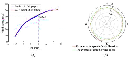
Figure 5.
(a) Average value of EWS with 50-year recurrence period of each wind direction in Shantou Yangdong wind farm; (b) EWS of each wind direction in 50-year recurrence period of Shantou Yangdong wind farm.
Table 3.
Distribution of wind speed and direction with 50-year recurrence at 100 altitudes of six OWF.
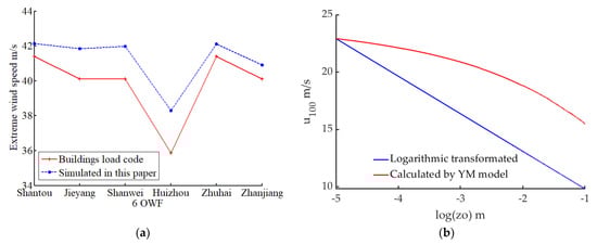
Figure 6.
(a) Comparison of EWS predicted in this paper with the result from building load code for six OWF under construction; (b) the Influence of z0 on wind speed at hub height from two different calculation method.
3.4. Prediction of EWS by Improving YM Model and Considering the Parametrization of Surface Roughness
In order to study the influence of z0 on the wind filed model, the other parameters of the YM typhoon field model are kept unchanged and select different z0 value to verify its influence on the simulated wind speed, and accordingly, recalculate wind speed at hub height by the Equation (9). The results are shown in Figure 6b. It can be seen that when z0 increase, the wind at the simulated height (100 m hub) became gentler, and the wind speed changes due to z0 changing through logarithmic rate transformation significantly greater than the result simulated from YM wind field. The main reason is that with the increase of wind surface roughness, the ground surface resistance to wind flow will increase, thus reducing the surface wind speed.
In this manuscript, Figure 7a reveals the comparison between z0 calculated by the above three empirical formula, IEC standard, and the measurement of Zhao et al. [50]. It can be seen from the figure that the roughness length of the sea surface would go up with the wind speeds; correspondingly, the resistance coefficient Cd would also increase, which is shown in Figure 7b. The result indicates that when the wind speeds less than 25 m/s, the difference of z0 and Cd calculated by the empirical formulas and obtained from the measurement is the least. However, accompanying the increase of wind speed, the roughness length calculated by the above three methods all deviates from the measured values, it increases violently. That means employing the methods mentioned above to calculate z0 without considering wind–wave coupling will hugely overestimate the sea surface roughness. In this way, the sea surface drag coefficient will also be overestimated, while the predicted measured wind speed will be underestimated on the contrary.
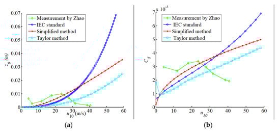
Figure 7.
(a) The comparison of z0 changed with wind speed calculated by different methods; (b) The comparison of changed with wind speed calculated by different methods.
To improve the accuracy of wind speed prediction, especially to realize the wind–wave coupling, the iterative method was adopted. That is, starting with the fixed value of z0 = 0.001 and using YM wind field model to calculate wind speed; then applying the wind sped to above three formula to get a corresponding new z0; and then introducing the new z0 to YM model to obtain the new wind speed. Thus, the iteration would stop when the deviation between the new and previous wind speeds is controlled within the specified range. In the simulation process, the above three methods all converge quickly.
The EWS prediction of Shantou Yangdong wind farm with different roughness length z0 calculating methods and measurement is shown in Figure 8. It reveals that the results of the four methods have little difference in the low recurrence period. With the increase of the recurrence period, both the EWS and the deviation increases. When calculating the 50-year recurrence period, the above four methods will underestimate the EWS. According to Taylor’s empirical formula, the predicted result is the closest to the measured value, with a minimum deviation of −3.9%. According to the IEC standard code, the deviation between the predicted result and the measured value is −11.4%, is the largest. The deviation between the method simplified by this paper and the measured value is −9.3%, but the method in this paper reduces computer time-consuming. When the fixed z0 = 0.001, the predicted wind speed will also be underestimated, the deviation is −4.2%. In this case, the wind–wave coupling relationship will be ignored; the result of predicted EWS offshore will be underestimated. To modify the EWS of the six OWF with 50-year recurrence period, Taylor’s formula of sea surface roughness length is applied to YM wind field when carrying out MCS. The fitted results are shown in Table 4. Among them, compared with fixed z0, the EWS of Huizhou Gangkou OWF has the most significant jump, with a maximum increase of 12.7%, and Shantou Yangdong OWF has the smallest increase of 3.8%. The results are consistent with the conclusions in the reference [20]: The wind–wave coupling increase the EWS.
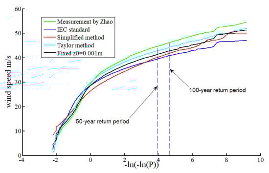
Figure 8.
The comparison of the fitting distribution of EWS value with z0 calculated by different methods.
Table 4.
Comparison of EWS with 50-year recurrence predicted by two methods for six OWF.
3.5. Summary and Discussion
To improve the reliability of EWS prediction for OWF, the meteorological data of typhoons are collected, and the key parameters are fitted by empirical distribution function. The fitting results show that the key parameters of typhoons in the southeast coast of China conform to the similar distribution. In this manuscript, the parameters setting and fitness of the YM model are verified by island observation station data. Taking the above OWF under construction in Guangdong Province as objects, and then comparing the EWS values predicted by the MCS with it by China national standard, respectively, the results demonstrate that OWF’s EWS is higher than that of a land wind farm because typhoon’s energy does not decay when passing through the OWF. A coupling method through exchanging roughness parameters in parametric wind field model and empirical wave formula is proposed. The influence of four roughness calculating methods used for wind speed prediction model is studied and verified by the measurement. It reveals that the wind-wave coupling has decrease effect on the simulated value when the wind speeds at a low level but contrary effect when at a high level. The critical wind speed is 25 m/s. Generally, only the maximum wind speeds will be selected when a typhoon is passing by the target site for predicting EWS. The values selected are usually greater than 25 m/s. If calculated according to a fixed value, then the surface roughness will be overestimated, leading to underestimate the EWS. By comparing the results of the four roughness parametrizations with the measurement, it can be found that the Taylor empirical formula is closest to the measured data. When predicting the EWS for offshore wind farm, the influence of wind–wave coupling should be considered seriously, especially for different sites. The diverse shape of the coastline will generate a significant influence on the wind-wave coupling, which eventually affects the EWS prediction precision. This should arouse our sufficient attention when we plan OWF: the EWS with great probability to exceed the design wind speed from many standards. Considering the results of this paper and wind turbine damaged disaster caused by typhoon, it is wise for decision-makers to choose wind turbines with a higher typhoon-resistant rating, especially in the southeast coastal offshore areas.
Author Contributions
Conceptualization, X.M., formal analysis, X.M., funding acquisition, Y.C., investigation, X.M., methodology, X.M. and Y.C., software, X.M., supervision, Y.C., validation, X.M., writing—original draft, X.M., W.Y. and Z.W., writing—review and editing, X.M., W.Y. and Z.W., project administration, Y.C. All authors have read and agreed to the published version of the manuscript.
Funding
The National Natural Science Foundation of China, grant number 51976113, Science and Technology Planning Project of Guangdong Province, grant number 2015B020240003, Science and Technology Planning Project of Huizhou City, grant number 2020SC0206015.
Institutional Review Board Statement
Not applicable.
Informed Consent Statement
Not applicable.
Data Availability Statement
Data is contained within the article.
Acknowledgments
The authors would like to thank all the scientists, engineers, and students who participated in the wind energy researching field.
Conflicts of Interest
All the authors declare no conflicts of interest.
References
- Song, L.L.; Mao, H.Q.; Qian, G.M. Analysis on the Wind Power by Tropical Cyclone. Taiyangneng Xuebao/Acta Energiae Solaris Sinica 2006, 27, 961–965. [Google Scholar]
- Ishihara, T.; Yamaguchi, A.; Takahara, K. An analysis of damaged wind turbines by typhoon Maemi. In Proceedings of the Sixth Asia-Pacific Conference on Wind Engineering (APCWE-VI), Seoul, Korea, 12–14 September 2005. [Google Scholar]
- Worsnop, R.P.; Lundquist, J.K.; Bryan, G.H. Gusts and shear within hurricane eyewalls can exceed offshore wind turbine design standards. Geophys. Res. Lett. 2016, 44, 6413–6420. [Google Scholar] [CrossRef]
- Guglielmo, D.; Filippo, P.; Flavio, P. Wind speed prediction for wind farm applications by Extreme Value Theory and Copulas. J. Wind. Eng. Ind. Aerodyn. 2015, 145, 229–236. [Google Scholar]
- IEC. IEC 61400-1: Edition Wind Turbines-Part 1: Design Requirements; IEC: Geneva, Switzerland, 2018; pp. 27–30. [Google Scholar]
- General Administration of Quality Supervision, Inspection and Quarantine and Standardization Administration of the People’s Republic of China. Wind Turbine Generator System under Typhoon Condition; GB/T31519; General Administration of Quality Supervision, Inspection and Quarantine and Standardization Administration of the People’s Republic of China: Beijing, China, 2016; p. 20.
- Ishihara, T.; Yamaguchi, A. Prediction of the extreme wind speed in the mixed climate region by using Monte Carlo simulation and measure-correlate-predict method. Wind Energ. 2015, 18, 171–186. [Google Scholar] [CrossRef]
- Zhao, L.; Ge, Y.J.; Song, L.L. Monte Carlo Simulation Analysis of Typhoon Extreme Value Wind Characteristics in Guangzhou. J. Tongji Univ. Nat. Sci. 2007, 35, 1034–1038. [Google Scholar]
- Xiao, Y.F.; Duan, Z.D.; Xiao, Y.Q. Typhoon wind hazard analysis for southeast China coastal regions. Struct. Saf. 2011, 33, 286–295. [Google Scholar] [CrossRef]
- Wang, J.C.; Quan, Y.; Gu, M. Assessment of the directional extreme wind speeds of typhoons via the Copula function and Monte Carlo simulation. Wind Struct. 2020, 30, 141–153. [Google Scholar]
- Fang, W.H.; Lin, W. A review on typhoon wind field modeling for disaster risk assessment. Prog. Phys. Geogr. 2013, 32, 852–867. [Google Scholar]
- Lin, N.; Emanuel, K.; Vanmarcke, E. 7 Physically-based hurricane risk analysis. In Extreme Natural Hazards, Disaster Risks and Societal Implications; Ismail-Zadeh, A., Urrutia Fucugauchi, J., Kijko, A., Takeuchi, K., Zaliapin, I., Eds.; Special Publications of the International Union of Geodesy and Geophysics; Cambridge University Press: Cambridge, UK, 2014; pp. 88–92. [Google Scholar]
- Dayal, K.; Cater, J.E.; Kingan, M.J. Evaluation of the WRF model for simulating surface winds and the diurnal cycle of wind speed for the small island state of Fiji. J. Phys. Conf. Ser. 2020, 1618, 1–12. [Google Scholar] [CrossRef]
- Ruiz-Salcines, P.; Salles, P.; Robles-Díaz, L.; Díaz-Hernández, G.; Torres-Freyermuth, A.; Appendini, C.M. On the Use of Parametric Wind Models for Wind Wave Modeling under Tropical Cyclones. Water 2019, 11, 2044. [Google Scholar] [CrossRef]
- Xu, Y.L. Windstorms and Cable-Supported Bridges. In Wind Effects on Cable-Supported Bridges; Xu, Y.L., Ed.; John Wiley & Sons Singapore Pte. Ltd.: Singapore, 2013; pp. 569–573. [Google Scholar]
- Vickery, P.J.; Twisdale, L.A. Wind-Field and Filling Models for Hurricane Wind-Speed Predictions. J. Struct. Eng. 1995, 121, 1700–1709. [Google Scholar] [CrossRef]
- Thompson, E.F.; Cardone, V.J. Practical modeling of hurricane surface wind fields. J. Waterw. Port Coast. Ocean Eng. 1996, 122, 195–205. [Google Scholar] [CrossRef]
- Batts, M.E.; Simiu, E.; Russell, L.R. Hurricane wind speeds in the United States. J. Struct. Div. 1980, 106, 2001–2016. [Google Scholar] [CrossRef]
- Yan, M.; Matsui, M.; Hibi, K. A numerical study of the wind field in a typhoon boundary layer. J. Wind. Eng. Ind. Aerodyn. 1997, 67, 437–448. [Google Scholar]
- Larsén, X.G.; Du, J.; Bolaños, R. Estimation of offshore extreme wind from wind-wave coupled modeling. Wind Energy 2019, 22, 1043–1057. [Google Scholar] [CrossRef]
- Charnock, H. A note on empirical wind-wave formulae. Q. J. R. Meteorol. Soc. 2010, 84, 443–447. [Google Scholar] [CrossRef]
- Edson, J.B.; Fairall, C.W. Similarity Relationships in the Marine Atmospheric Surface Layer for Terms in the TKE and Scalar Variance Budgets*. J. Atmos. Sci. 1998, 55, 2311–2328. [Google Scholar] [CrossRef]
- Taylor, P.K.; Yelland, M.J. The Dependence of Sea Surface Roughness on the Height and Steepness of the Waves. J. Phys. Oceanogr. 2000, 31, 572–590. [Google Scholar] [CrossRef]
- Zijlema, M.; Vledder, G.P.V.; Holthuijsen, L. Bottom friction and wind drag for wave models. Coast. Eng. 2012, 65, 19–26. [Google Scholar] [CrossRef]
- Edson, J.B.; Jampana, V.; Weller, R. On the Exchange of Momentum over the Open Ocean. J. Phys. Oceanogr. 2013, 43, 1589–1610. [Google Scholar] [CrossRef]
- Fan, Y.; Lin, S.J.; Held, I.M. Global ocean surface wave simulation using a coupled atmosphere–wave model. J. Clim. 2012, 25, 6233–6252. [Google Scholar] [CrossRef]
- Liu, B.; Liu, H.; Xie, L. A Coupled Atmosphere-Wave-Ocean Modeling System: Simulation of the Intensity of an Idealized Tropical Cyclone. Mon. Weather Rev. 2011, 139, 132–152. [Google Scholar] [CrossRef]
- Janssen, P.; Lionello, P.; Zambresky, L. On the interaction of wind and waves. Philos. Trans. R. Soc. Lond. Ser. Math. Phys. Sci. 1989, 329, 289–301. [Google Scholar]
- Jensen, R.E.; Cardone, V.J.; Cox, A.T. Performance of Third Generation Wave Models in Extreme Hurricanes. In Proceedings of the 9th International Workshop of Wave Hindcasting and Forecasting, Victoria, BC, Canada, 24–29 September 2006. [Google Scholar]
- Chalikov, D.V.; Makin, V.K. Models of the wave boundary layer. Bound.-Layer Meteorol. 1991, 56, 83–99. [Google Scholar] [CrossRef]
- Makin, V.K.; Kudryavtsev, V.N.; Mastenbroek, C. Drag of the sea surface. Bound.-Layer Meteorol. 1995, 73, 159–182. [Google Scholar] [CrossRef]
- Drost, E.J.F.; Lowe, R.J.; Ivey, G.N. The effects of tropical cyclone characteristics on Australia’s North West region. Cont. Shelf Res. 2017, 139, 35–53. [Google Scholar] [CrossRef]
- Guo, Y.; Hou, Y.; Liu, Z. Risk Prediction of Coastal Hazards Induced by Typhoon: A case study in the Coastal Region of Shenzhen, China. Remote Sens. 2020, 12, 1731. [Google Scholar] [CrossRef]
- Yan, Z.D.; Liang, B.C.; Wu, G.X. Ultra-long return level estimation of extreme wind speed based on the deductive method. Ocean Eng. 2020, 197, 106900–106912. [Google Scholar] [CrossRef]
- Cappé, O.; Godsill, S.J.; Moulines, E. An Overview of Existing Methods and Recent Advances in Sequential Monte Carlo; IEEE: Piscataway, NJ, USA, 2007; Volume 95, pp. 899–924. [Google Scholar]
- MathWorks. Available online: https://www.mathworks.com/help/stats/mhsample.html (accessed on 1 January 2021).
- Lettau, H.H. Physical and meteorological basis for mathematical models of urban diffusion processes. In Proceedings of Symposium on Multiple-Source Urban Diffusion Models; Arthur, C.S., Ed.; US Environmental Protection Agency: Durham, NC, USA, 1970; pp. 2.1–2.26. [Google Scholar]
- Helliwell, N.C. Wind over London. In Proceedings of the Wind Effects on Buildings and Structures; Saikon Co.: Tokyo, Japan, 1971; pp. 23–32. [Google Scholar]
- Kondo, J.; Yamazawa, H. Aerodynamic roughness over an inhomogeneous ground surface. Bound.-Layer Meteorol. 1986, 35, 331–348. [Google Scholar] [CrossRef]
- Simiu, E. Equivalent static wind load for tall building design. In Proceedings of the 4th International Conference, Munich, Germany, 26–30 July 2004. [Google Scholar]
- Wu, J. Wind stress and surface roughness at air-sea interface. J. Geophys. Res. 1969, 74, 444–455. [Google Scholar] [CrossRef]
- IEC. IEC 61400–3 Edition 1.0: Design Requirements for Offshore Wind Turbines Eoliennes; IEC: Geneva, Switzerland, 2019; pp. 30–40. [Google Scholar]
- Typhoon Network of the China Central Meteorological Station. Available online: http://typhoon.nmc.cn/web.html (accessed on 1 March 2020).
- Holland, G.J. An analytic model of the wind and pressure profiles in hurricanes. Mon. Weather Rev. 1980, 108, 1212–1218. [Google Scholar] [CrossRef]
- Jiang, Z.H.; HUA, F.; Qu, P. A New Scheme for Adjusting the Tropical Cyclone Parameter. Adv. Marine Sci. 2008, 26, 5–11. [Google Scholar]
- Ying, M.; Zhang, W.; Yu, H. An Overview of the China Meteorological Administration Tropical Cyclone Database. J. Atmos. Ocean. Technol. 2014, 31, 287–301. [Google Scholar] [CrossRef]
- SA/SNZ (Standard Australian/Standard New Zealand). Structural Design Actions—Wind Actions AS/NZS 1170.2-2002; Standards Australia and Standards New Zealand: Sydney, Australia; Wellington, New Zealand, 2002; pp. 6–20.
- Harper, B.A.; Kepert, J.D.; Ginger, J.D. Guidelines for Converting between Various Wind Averaging Periods in Tropical Cyclone Conditions; No. 1555; WMO: Geneva, Switzerland, 2010; pp. 4–16. [Google Scholar]
- MOHURD (Ministry of Housing and Urban-Rural Development of the People’s Republic of China). Load Code for the Design of Building Structures GB 50009-2012; MOHURD: Beijing, China, 2012; pp. 30–50.
- Zhao, Z.K.; Liu, C.X.; Li, Q.; Dai, G.-F.; Song, Q.-T.; Lv, W.-H. Typhoon air-sea drag coefficient in coastal regions. J. Geophys. Res. Oceans 2015, 120, 716–727. [Google Scholar] [CrossRef]
Publisher’s Note: MDPI stays neutral with regard to jurisdictional claims in published maps and institutional affiliations. |
© 2021 by the authors. Licensee MDPI, Basel, Switzerland. This article is an open access article distributed under the terms and conditions of the Creative Commons Attribution (CC BY) license (http://creativecommons.org/licenses/by/4.0/).