Modeling Water Droplet Freezing and Collision with a Solid Surface

Abstract

Water droplets released from the sea surface represent one of the major causes of ice accretion on marine vessels. A one-dimensional model of the freezing of a spherical water droplet moving in cold air was developed. The crystallization model allows one to obtain an analytical solution if a uniform temperature distribution over the liquid’s core is assumed. The model was validated using STAR CCM+ Computational fluid dynamics (CFD) code. A collision of a partially frozen droplet with a solid wall assuming the plastic deformation of an ice crust was also considered. The ratio of the crust deformation to the crust thickness was evaluated. It was assumed that if this ratio were to exceed unity, the droplet would stick to the wall’s surface due to ice bridge formation caused by the water released from the droplet’s core.

1. Introduction

Droplets may be generated on water surfaces under windy conditions. As they are transported with cold air, the droplets rapidly cool and then either partially or entirely solidify. If it collides with a solid wall, such a partially frozen droplet may either stick to the wall’s surface or bounce off. Particles sticking to offshore structures and ships’ surfaces may eventually lead to significant ice accretion, representing a severe problem for further equipment exploitation [1].

The rate of the ice accretion depends mainly on the following factors [2]: (1) wind speed; (2) surface-wave conditions; (3) ambient air temperature; (4) air humidity; (5) water surface temperature; (6) water salinity; (7) angle of droplet-surface interaction; and (8) properties of the vessel’s (equipment’s) surface, its special orientation, and its speed. Additional loads caused by ice formations alter the vessel’s or stationary structure’s center of mass, increasing construction instability risks. Another important problem is the erosion of floating wind turbines.

There is a lack of statistical data for accurate analyzing the accretion problem [1]. Therefore, a mathematical model can be a useful tool for ice formation forecasting. A number of ice accretion models have been reported for different objects, such as aircraft [3,4], electrical power lines [5,6], and marine equipment [7]. The ice accretion process involves the modeling of several sub-processes. First, a droplet’s generation from a water surface and interaction with wind flow have to be modeled. A model should properly forecast droplet generation frequency, size, and velocity distribution. Second, the transportation of the droplet through the ambient air, accompanied by cooling and freezing, should also be modeled. Finally, multiple interactions of droplets with a solid wall and ice layer formation and growth on that wall have to be forecasted. To the best of our knowledge, there are no ice accretion simulation tools that account for all of the aforementioned sub-processes [8]. Moreover, the majority of the known models of these sub-processes are computationally expensive, limiting their employment as components of an efficient computational tool. The present work suggests a preliminary engineering approach to solving the second and third groups of the formulated problems.

We limit our considerations to the development of a simple model of the cooling of a droplet, its partial solidification, and its further interaction with the solid wall surface. To a great extent, our work is in line with the research of [9], who developed a model of the collision of an ice particle with a wall, which has an implied applicability to the modeling of ice accretion. The model presented below is simple and suitable only for an approximate analysis of ice accretion. The simplicity of the model is justified by our intention to incorporate this model into a detailed CFD code developed for 3D simulations of the entire ice accretion process that will be adjusted, verified, and validated with experimental data.

2. Modeling

The model consists of two sub-models: (a) droplet cooling and ice crust growth; (b) breakage of a partially frozen droplet caused by its collision with the solid surface.

2.1. Droplet Cooling and Solidification

Let us assume that a droplet maintains a spherical shape during its motion. This assumption is justified by the relatively small sizes of droplets generated on the surface of seawater. Seawater is usually contaminated with different impurities. Therefore, it is possible to assume that a droplet’s surface is rigid (immobile), and the circulation motion inside a droplet can be neglected [10]. A small-sized droplet generated in the air is cooled due to convective heat transfer. Such a droplet usually rotates with an unknown and non-constant angular velocity. Due to this uncertainty, in engineering applications, the droplet–air heat transfer coefficient is calculated with empirical correlations (e.g., [11]). Assuming that the heat flux through the droplet’s surface is uniform, we can conclude that the heat transfer inside the droplet can be described by the one-dimensional equation of heat conduction for a sphere. Prior to the solidification of a droplet, its surface should be cooled to the crystallization temperature. To describe the cooling of a liquid droplet, we use the heat conduction equation, which is formulated in the dimensionless form [12]:

$$\frac{\partial \theta (\xi ,\tau )}{\partial \tau }=\frac{{\partial }^2\theta (\xi ,\tau )}{\partial {\xi }^2}+\frac{\partial \theta (\xi ,\tau )}{\partial \xi }\frac{2}{\xi },$$

(1)

where $\theta (\xi ,\tau )=(T(\xi ,\tau )-T_{\infty })/(T_{cr}-T_{\infty })$ is the dimensionless temperature, T is the temperature, $T_{\infty }$ is the ambient air temperature, $T_{cr}$ is the water crystallization (freezing) temperature, $\tau ={\alpha }_{w}t/R_0^2$ is the dimensionless time, t is the time, $R_0$ is the droplet radius, ${\alpha }_w=k_w/\left({\rho }_w{c}_w\right)$ is the water’s thermal diffusivity, $k_w$ is the water’s thermal conductivity, ${\rho }_w$ is the water’s density, $c_w$ is the water’s specific heat capacity, $\xi =r/R_0$ is the dimensionless radial coordinate, and r is the radial coordinate.

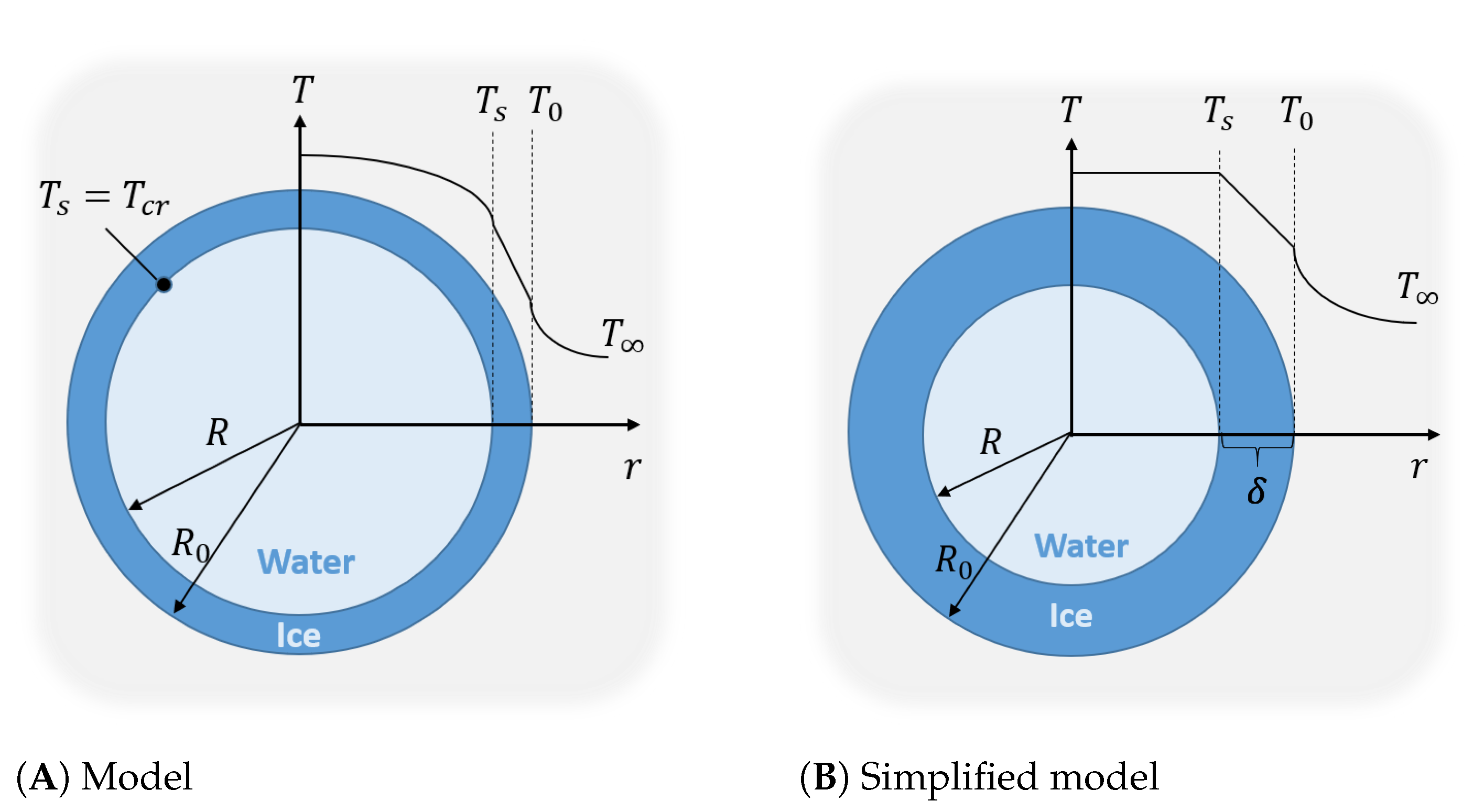
Equation (1) is applicable until the moment when the temperature at the droplet’s surface, $T_s$, reaches the water’s freezing temperature. After that, the solid crust starts growing toward the droplet’s center. This solidification process represents a well-known Stefan problem. A diagram illustrating this process is shown in Figure 1A. The heat conduction inside a shrinking liquid core that is coated with a solid crust of increasing thickness is described by the heat conduction equation, which is formulated in coordinates normalized by the radius of the liquid core. Equation (1) can be converted into the heat conduction equation for the liquid core, accounting for a decreasing radius, through the following coordinate transformation [13]:

$$(t,r)\to (\tau ,\xi );\frac{\partial }{\partial t}=\frac{{\alpha }_w}{R_0^2}\left(\frac{\partial }{\partial \tau }-\frac{dln\overline{R}}{d\tau }\xi \frac{\partial }{\partial \xi }\right);\frac{\partial }{\partial r}=\frac{1}{R\left(t\right)}\frac{\partial }{\partial \xi },$$

(2)

where $\xi =r/R$ is the dimensionless radial coordinate, R is the liquid core’s radius, and $\overline{R}\left(\tau \right)=R/R_0$ is the dimensionless radius of the liquid core.

This transformation leads to the following equation:

$$\frac{\partial \theta (\xi ,\tau )}{\partial \tau }=\frac{1}{{\overline{R}}^2\left(\tau \right)}\left[\frac{\partial \theta (\xi ,\tau )}{\partial \xi }\left(\frac{d\overline{R}}{d\tau }\xi \overline{R}\left(\tau \right)+\frac{2}{\xi }\right)+\frac{{\partial }^2\theta (\xi ,\tau )}{\partial {\xi }^2}\right].$$

(3)

We would like to emphasize that Equation (3) was successfully employed in [14] for modeling the heat transfer inside an oil sand lump digested in a hot pipeline water flow.

The liquid core’s shrinkage rate, which is caused by ice crust formation, is derived from the heat balance at the liquid core/solid crust boundary formulated for a small time lapse $dt$. During $dt$, the heat rejected from the liquid core’s surface due to conduction through the solid crust is spent on both solidification of a thin spherical layer of the thickness $dR$ and on cooling of the liquid core by heat conduction through the liquid. The only assumption employed for the derivation of the shrinking rate equation is the steady-state heat conduction through the solid crust. This assumption is justified by both a rather small ice crust thickness, which is caused by the short time of droplet motion in cold air, and the relatively high thermal diffusivity of ice. After conducting routine math, the obtained heat balance equation is transformed into the dimensionless equation for the radius reduction rate of the unfrozen core as follows:

$$\frac{d\overline{R}}{d\tau }=-Ste\frac{c_w{\rho }_w}{c_s{\rho }_s}\left[\frac{k_a}{k_w}\frac{Nu}{Bi\overline{R}(1-\overline{R})+2{\overline{R}}^2}+\frac{1}{\overline{R}}\frac{\partial \theta }{\partial \xi }\right],$$

(4)

where $Ste=\frac{c_s(T_{cr}-T_{\infty })}{H_f}$ is the Stefan number, $H_f$ is the latent heat of crystallization, $c_s$ is the ice’s specific heat capacity, ${\rho }_s$ is the ice’s density, $Bi=2R_{0}h/k_s$ is the droplet’s Biot number, $k_s$ is the ice’s thermal conductivity, h is the droplet–ambient-air convective heat transfer coefficient, $Nu=2R_{0}h/k_a$ is the droplet’s Nusselt number, and $k_a$ is the air’s thermal conductivity.

In the present work, the Nusselt number was calculated with the well-known Ranz–Marshal correlation: $Nu=2+0.6R{e}^{1/2}P{r}^{1/3}$ [11], where $Re=2{\rho }_a{R}_{0}U/{\mu }_a$ is the droplet’s Reynolds number, U is the droplet–air relative velocity, ${\rho }_a$ is the density of air, ${\mu }_a$ is the air’s dynamic viscosity, $Pr=c_a{\mu }_a/k_a$ is the air’s Prandtl number, and $c_a$ is the air’s specific heat capacity.

The initial condition required for the solution of the equation of droplet cooling, Equation (1), is the known water temperature uniformly distributed over the droplet volume. The first boundary condition in the droplet center is as follows:

$${\left(\frac{\partial \theta }{\partial \xi }\right)}_{\xi =0}=0.$$

(5)

Note that the first boundary condition is also the same for Equation (3). The second boundary condition for Equation (1) is obtained by equating the convection heat flux out of the droplet’s surface to the conduction flux toward this surface, and it is formulated as follows:

$${\left(\frac{\partial \theta }{\partial \xi }\right)}_{\xi =1}=-0.5Nu\frac{k_a}{k_w}\theta (1,\tau ).$$

(6)

The second boundary condition for Equation (3) expresses the equality of the temperature at the liquid core’s boundary to the water’s crystallization temperature, i.e.,

$$\theta (1,\tau )=1.$$

(7)

Thus, Equations (1)–(7) allow the calculation of both the cooling and freezing processes for a droplet moving in cold air.

Assuming that, at the initial moment in time, the temperature over the droplet’s liquid core is uniform and equal to the crystallization temperature (i.e., $\partial \theta /\partial \xi =0$), Equation (4) can be solved analytically. A diagram illustrating this simplified case is shown in Figure 1B. The analytical equation relating the dimensionless time and the solid crust’s thickness has the following form [15]:

$$\tau =\frac{1}{2Ste}\frac{{\rho }_s}{{\rho }_w}\frac{{\alpha }_w}{{\alpha }_s}\left[1-{\left(1-\frac{\delta }{R_0}\right)}^2+\frac{2}{3}\left(\frac{2}{Bi}-1\right)\left(1-{\left(1-\frac{\delta }{R_0}\right)}^3\right)\right],$$

(8)

where ${\alpha }_s=k_s/\left({\rho }_s{c}_s\right)$ is the ice’s thermal diffusivity and $\delta$ is the ice crust’s thickness.

Although at the normal conditions, the ice’s density is about 9% lower than the water’s density, for the sake of simplicity, we assume ${\rho }_s/{\rho }_w=1$. This simplification weakly affects the modeling results.

The model equations (Equations (1), (3), and (4)) were solved numerically using an explicit finite difference technique. A Matlab code was developed for this purpose. The code demonstrated rapid convergence and independence of the solution on the chosen radial and time steps ($d\xi =0.02$ and $dt={10}^{-5}$ s, respectively). Note that for the one-dimensional heat conduction problem, the stability of an explicit numerical method is determined by the Fourier number formulated for a single integration cell [16]. If this criterion is smaller than 0.5, the numerical method is stable. This condition has been satisfied for the computations conducted within the present work. To further support the correctness of the model validation presented here, we would like to emphasize again that the model of droplet solidification proposed in the present work has a single assumption that differentiates it from the accurate one-dimensional model that was solved and validated by different authors [15,17]. This assumption is the steady-state heat transfer through the ice crust, which is justified by both the small crust thickness and high thermal diffusivity of ice. We estimated the Fourier number for the crust, assuming that its characteristic size was equal to the crust’s thickness. It turned out that the Fourier numbers corresponding to the crust thickness range considered in the present work are almost always below the critical value, 0.1, indicating the nearly immediate formation of a uniform temperature profile across the crust if the liquid core is absent. This result means that heat conduction through the crust is practically the steady state process. Thus, the model for forecasting the thin ice crust growth suggested in this work has to provide results that are very close to those calculated using the standard (accurate) model [15]. Therefore, the model validation given here is primarily aimed at validating not the model itself, but the numerical code developed.

The presented cooling/freezing model was validated by comparing the calculated results with those computed using the commercial STAR CCM+ CFD code. The model incorporated into this code assumes that solidification occurs not at a single temperature value, but within a defined temperature range [18]. Note that this modeling approach was originally developed for metal alloys. According to this model, a mixture of solid and liquid is formed during the crystallization process. A solid-phase volume fraction corresponding to a certain temperature is assumed to be known. This model was meticulously validated [19]. To apply it to the ice crust formation calculation, we assumed a very small range for the solidification temperature, 0.002 °C. The volume fraction of ice was linearly interpolated within this range.

The STAR CCM+ simulations were conducted in the three-dimensional formulation. The initial and boundary conditions for the CFD model were the same as those for the developed model. The uniform mesh was employed for all of the computations. The mesh size was assumed to be equal to the initial mesh size used in the Matlab code. The same time step was employed for both codes.

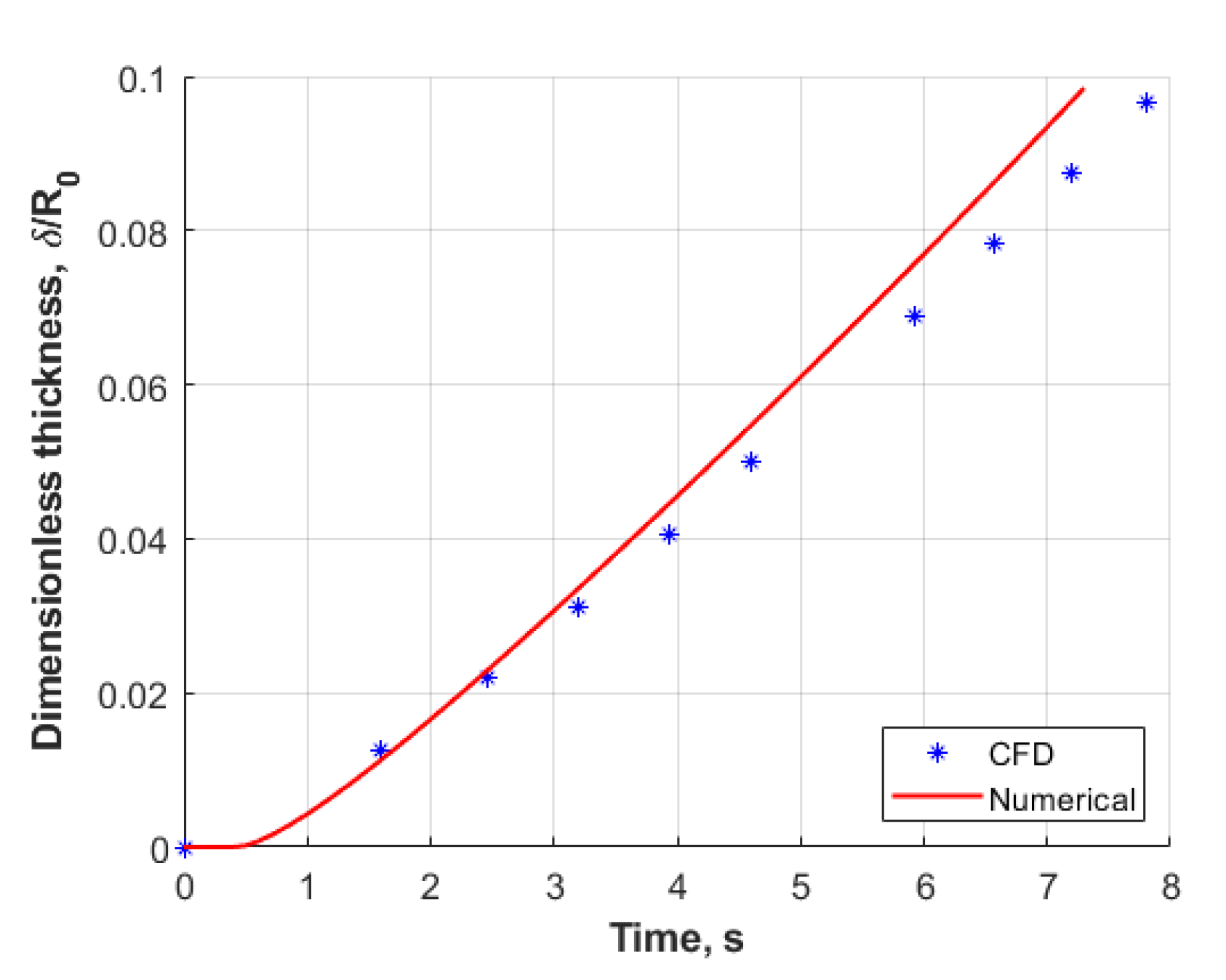
In Figure 2, we show the dimensionless crust thickness vs. time, comparing the computed results using the STAR CCM+ CFD code with the results calculated using the in-house engineering code developed based on the model presented here. The computations were done for a droplet with a 2 mm diameter. The initial droplet temperature was assumed to be $T_0$ = 3 °C and the ambient air temperature was assumed to be $T_{\infty }=-20$ °C. The air–droplet heat transfer coefficient was calculated, assuming that the droplet–air relative velocity was equal to the droplet’s terminal velocity. The properties of the water, ice, and air used for the calculations are given in

Table 1. Physical properties of water, ice, and air used for the computations.

Physical Property	Unit	Water	Ice	Air
Density	kg/m3	1000	1000	1.292
Thermal conductivity	W/(m·K)	0.57	2.2	0.024
Specific heat capacity	J/(kg·K)	4217	2108	1003

. These data were obtained at a constant temperature equal to 0 °C [20].

One can see that the results of computations by the different models are relatively close to each other. The slightly faster growth of the ice crust forecasted by the Matlab code was probably caused by the assumption of the steady-state heat transfer through this crust. The difference between the computational results increases with an increase in the crust thickness: The thicker the crust is, the longer the time needed to obtain the steady-state temperature distribution across the crust assumed in the Matlab code. The larger the deviation from the steady-state assumption, the larger the error caused by this simplification. Note that the Matlab code’s numerical inaccuracy is excluded from the present analysis due to the proven independence of the generated data on both the spatial and time steps. It is possible to affirm that the results presented in Figure 2 support our conclusion that the developed ice crust formation model is sufficiently accurate for practical calculations. We would like to stress that further model validation with experimental data is unfeasible for two reasons: (1) It has been proven that the developed model provides results close to those produced by the accurate model for a small crust thickness; (2) there are no known experimental data on droplet freezing that were obtained while monitoring the thickness of a thin ice crust.

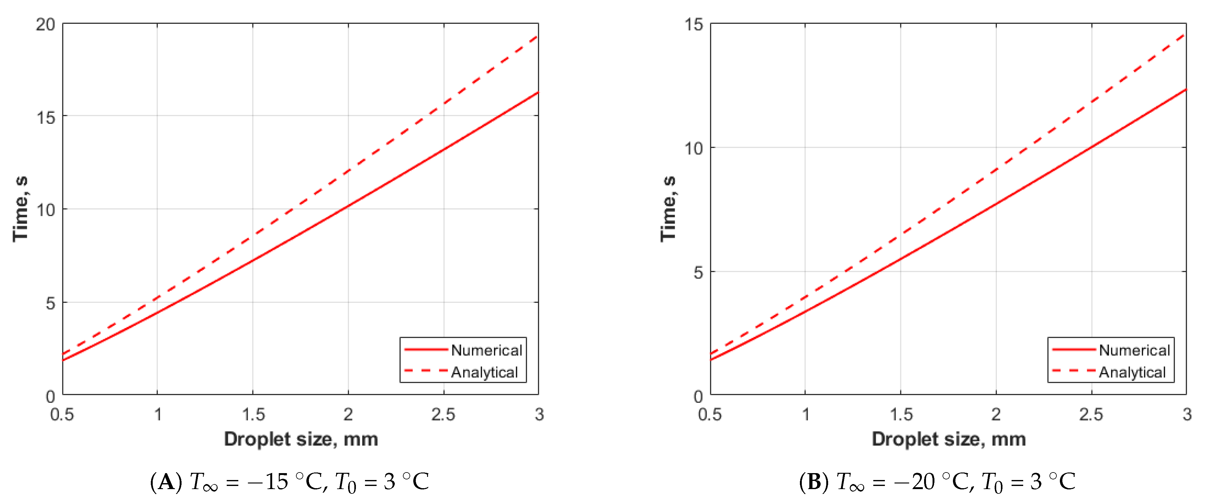
In Figure 3, we compare the numerical solution obtained by the developed Matlab code with the analytical solution. The initial droplet temperature was assumed to be $T_0$ = 3 °C. For Figure 3A, the ambient air temperature was set equal to $T_{\infty }$ = −15 °C, and for Figure 3B, it was set to $T_{\infty }$ = −20 °C. All of the calculations for Figure 3 were conducted with the assumption that the obtained crust thickness, $\delta$, was equal to $10\%$ of the droplet’s radius. Note that the curve showing the analytical solution was obtained as a sum of the crystallization time, which was calculated by Equation (8), and the cooling time, ${\tau }_c$, which was estimated assuming a uniform droplet temperature [21]. The dimensionless cooling time is calculated as follows:

$${\tau }_c=\frac{2}{3}\frac{ln\theta \left(1\right)}{Nu}.$$

(9)

Our calculations showed that the cooling time stage is relatively short for the droplet size range considered. The crust formation times calculated by the analytical equation are close to those computed by the Matlab code; however, the deviations of the analytical solution from the numerical one increase with an increase in the droplet size. This observation is explained as follows. The analytical solution does not account for heat conduction through the liquid core during the solidification process. The larger the droplet size, the higher the corresponding heat conduction flux because larger droplets are characterized by higher temperature gradients; therefore, the error associated with neglecting the conduction flux in the liquid core increases with an increase in the droplet size. Nevertheless, the analytical equations (Equations (8) and (9)) are accurate enough to be used for practical estimations of the crust thickness vs. time if the droplet size is relatively small.

2.2. Particle–Wall Collision

We would like to emphasize that rapid growth of the ice crust is accompanied with the formation of different defects (e.g., micro-cracks) and, consequently, is characterized by a relatively low strength. There are numerous research works on solid particle–wall collisions. It is worth mentioning a couple of recent experimental works [22,23] where ice particle–wall interactions were studied.

Our estimations showed that a collision of a droplet coated by an ice crust with a wall is usually associated with plastic deformation of the ice. Elastic deformation corresponds to a very low collision velocity and, therefore, does not represent a practical interest.

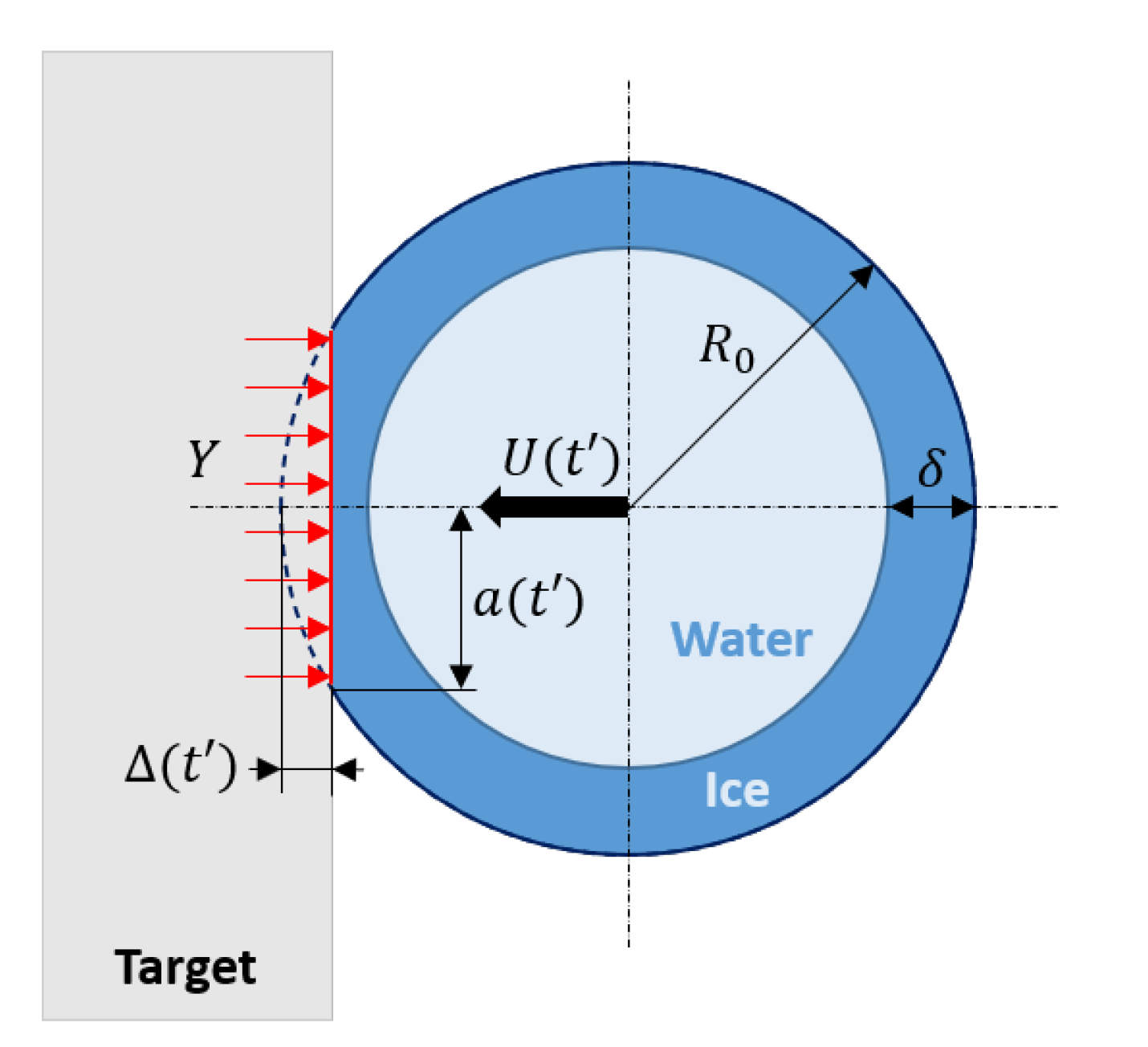
The process of a collision of a partially frozen droplet with a solid surface can be modeled using the approach suggested in [9]. The corresponding diagram is shown in Figure 4. We limit our analysis to normal collisions, i.e., we assume that the droplet’s velocity is normal to the wall. However, this approach can also be employed for oblique collisions if a velocity component that is normal to the wall is used.

The particle’s displacement during the plastic deformation of the solid crust is described by the following equation [9]:

$$\frac{d^{2}z}{d{t^{\prime }}^2}=-\frac{\pi Ya\left(z\right)}{R_0{\rho }_{w}V\left(z\right)},$$

(10)

where $z=\Delta /R_0$ is the dimensionless droplet displacement during an interaction with the wall surface, $\Delta$ is the droplet displacement, Y is the ice’s yield strength (assumed to be $Y=5.2$ MPa [24]), $a\left(z\right)=R_0\sqrt{z(2-z)}$ is the radius of the particle–wall contact area, and $V\left(z\right)=\frac{\pi R_0^3}{3}{(2-z)}^2(1+z)$ is the volume of the uncrushed particle part. Note that the time count, $t^{\prime }$, for this equation starts from the moment at which the particle touches the wall.

The initial condition for Equation (10) is the known particle velocity at the moment of touching the wall, $U_0$, which is written as:

$$z=0,\frac{dz}{d{t}^{\prime }}=\frac{U_0}{R_0}.$$

(11)

Equation (10) has the analytical solution [9], where the maximum dimensionless center displacement, $z_{max}=\Delta \left(t_{end}^{\prime }\right)/R_0$, is expressed as:

$${(2-z_{max})}^2(1+z_{max})=4exp\left(-\frac{{\rho }_w{U}_0^2}{2Y}\right),$$

(12)

where $t_{end}^{\prime }$ is the collision duration.

In the present work, the equation describing plastic deformation of the ice crust was utilized to evaluate the probability of a particle sticking to the wall in the following way. It was assumed that if the deformation $\Delta$ is smaller than the crust thickness, the droplet bounces from the wall. In contrast, if the deformation exceeds the crust thickness, the droplet sticks to the wall due to adhesion caused by the immediate formation of an ice bridge induced by water released from the droplet’s core.

3. Results and Discussion

To analyze the interaction of a partially solidified droplet with a wall, we introduced the critical velocity, which indicates the equality of the plastic droplet’s deformation and the ice crust’s thickness. We assume that if the droplet velocity exceeds the critical velocity, the droplet sticks to the wall.

For our simplified analysis, we assume that the droplet velocity, representing a droplet–wall interaction, is equal to the normal-to-the-wall component of the absolute droplet velocity.

The analysis, which is illustrated in Figure 5, is based on the following computational algorithm for the critical droplet velocity: (1) The droplet diameter and traveling duration are given, whilst the droplet velocity is assumed; (2) the temperature distribution along the droplet radius is calculated numerically by Equation (1) until the moment when the temperature at the droplet surface is equal to the water crystallization temperature; (3) then, both the temperature distribution along the liquid core radius and the crust thickness are calculated by Equations (3) and (4), respectively; (4) the crust deformation is calculated by Equation (12) and compared to the crust thickness; (5) if the crust deformation is smaller than the crust thickness, the droplet velocity is increased, and if it is larger, the droplet velocity is decreased; (6) steps 2–5 are repeated until the difference between the crust thickness and its deformation becomes smaller than an acceptable error assumed in advance, which means that the droplet velocity reached the critical value.

In Figure 5A–D, we show the dependence of the critical droplet velocity on the droplet size for the different traveling times in ambient air. In each figure, (A)–(D) correspond to a certain air temperature.

Note that it was assumed that the droplet–air relative velocity is constant and equal to the terminal droplet velocity for all of the computations.

It can be seen that for the fixed traveling time, the critical velocity after an initial rapid reduction slowly decreases with an increase in the droplet size. This observation is explained as follows. First, the smaller the droplet size, the faster both the cooling and the further increase in the ice crust’s thickness. The thicker the crust, the higher the critical velocity. Second, the smaller the droplet size, the lower the droplet inertia, leading to a smaller collision-induced deformation than the deformation of a larger particle at the same collision velocity. Both of these factors lead to the strong effect of the droplet size on the critical collision velocity. This effect is rapidly reduced with an increase in the droplet size because the relative contributions of these factors are decreased. An increase in the critical velocity with an increase in the droplet traveling time is obvious. The longer the time, the thicker the crust; therefore, a higher velocity is required to break it. A reduction in the ambient air temperature, which is different for Figure 5A–D, leads to faster droplet cooling and crust growth. Therefore, an ambient temperature drop causes an upward shift of the curves due to the increase in the droplet velocities required to break thicker crusts. It is important to emphasize that the ranges of the critical velocity values obtained in the calculations, which are illustrated by Figure 5, are realistic, i.e., they correspond to actual wind speeds. Our results are also in agreement with the field data [25], showing that an increase in the wind speed leads to an increase in the ice accretion rate. The computational results also do not contradict to the field data [25], according to which the highest ice accretion rate is observed in the ambient temperature range of about −10 to −5 °C. The same set of field data show that the ice accretion rate decreases with a decrease in temperature, which can be explained by the corresponding increase in the critical droplet velocity (see Figure 5). The decrease in the ice accretion rate observed at ambient air temperatures higher than −5 °C [25] can be explained by a corresponding reduction in the strength of the ice bridge that glues partially frozen droplets to the wall surface. The suggested engineering approach for evaluating the sticking probability of a partially frozen droplet to the solid wall surface allowed us to evaluate the minimum velocity that indicates this event. This approach was reduced to solving relatively simple equations. Moreover, the rather accurate analytical solution of droplet solidification enabled us to avoid solving the partial differential equation of heat conduction (Equations (1)–(3)). As a result, the developed modeling approach requires one to solve several analytical equations (Equations (8), (9), and (12)), which do not require significant computational resources. Thus, the modeling approach looks suitable for incorporation into the three-dimensional CFD code for computations of the generation of multiple droplets from a sea surface and their transport to structures that are expected to be coated with ice. Finally, we would like to emphasize that although the suggested approach to modeling droplet sticking probability looks oversimplified, it represents a reasonably justified step toward the development of a comprehensive CFD-based model of ice accretion.

4. Conclusions

An approach for evaluating the sticking probability of a partially frozen spherical droplet colliding with a rigid wall has been developed. This model includes two sub-models: (1) cooling of a droplet and formation of an ice crust coating the liquid droplet’s core; (2) droplet–solid wall interaction. The formation of an ice crust was modeled by solving the heat conduction equation formulated in the moving coordinate system. A collision of the partially frozen droplet with the wall was modeled with the assumption of plastic deformation of the ice crust. It was assumed that the droplet sticks to the wall if the ice crust deformation exceeds the crust thickness. The critical droplet velocity, indicating the minimum droplet velocity leading to the sticking event, was introduced. The critical velocity was employed as a criterion for illustrating the effects of the droplet size, the total time required for droplet cooling and solidification, and the ambient air temperature on the droplet sticking to the wall. The computed dependencies of the critical velocity on the different factors allow the explanation of the corresponding ice accretion rate trends observed in the field.

Although the developed modeling approach is very approximate, it has the potential to be efficiently incorporated into a prospective three-dimensional CFD code for simulations of ice accretion on different structures as a subroutine. It is also possible to tune our simplified model for more detailed models if improved accuracy is needed.

References

1. Minsk, L.D. Ice Accumulation on Ocean Structures; Number 77; Department of Defense, Department of the Army, Corps of Engineers, Cold Regions Research and Engineering Laboratory: Hanover, NH, USA, 1977. [Google Scholar]
2. Dehghani, S.; Naterer, G.; Muzychka, Y. Droplet size and velocity distributions of wave-impact sea spray over a marine vessel. Cold Reg. Sci. Technol. 2016, 132, 60–67. [Google Scholar] [CrossRef] [Green Version]
3. Papadakis, M.; Rachman, A.; Wong, S.C.; Yeong, H.W.; Hung, K.E.; Vu, G.T.; Bidwell, C.S. Water Droplet Impingement on Simulated Glaze, Mixed, and Rime Ice Accretions; NASA STI Report Series: Hanover, MD, USA, 2007. [Google Scholar]
4. Cao, Y.; Huang, J.; Yin, J. Numerical simulation of three-dimensional ice accretion on an aircraft wing. Int. J. Heat Mass Transf. 2016, 92, 34–54. [Google Scholar] [CrossRef]
5. Fu, P.; Farzaneh, M.; Bouchard, G. Two-dimensional modelling of the ice accretion process on transmission line wires and conductors. Cold Reg. Sci. Technol. 2006, 46, 132–146. [Google Scholar] [CrossRef]
6. Fu, P.; Farzaneh, M. A CFD approach for modeling the rime-ice accretion process on a horizontal-axis wind turbine. J. Wind. Eng. Ind. Aerodyn. 2010, 98, 181–188. [Google Scholar] [CrossRef]
7. Dehghani-Sanij, A.; Dehghani, S.; Naterer, G.; Muzychka, Y. Marine icing phenomena on vessels and offshore structures: Prediction and analysis. Ocean. Eng. 2017, 143, 1–23. [Google Scholar] [CrossRef]
8. Mintu, S.; Molyneux, D.; Oldford, D. State-of-the-Art Review of Research on ice Accretion Measurements and Modelling. In Proceedings of the Arctic Technology Conference. Offshore Technology Conference, Houston, TX, USA, 24 October 2016. [Google Scholar]
9. Roisman, I.; Tropea, C. Impact of a crushing ice particle onto a dry solid wall. Proc. R. Soc. A Math. Phys. Eng. Sci. 2015, 471, 20150525. [Google Scholar] [CrossRef] [Green Version]
10. Levich, V.G. Physicochemical Hydrodynamics; Prentice-Hall Inc.: Upper Saddle River, NJ, USA, 1962. [Google Scholar]
11. Ranz, W.; Marshall, W. Evaporation from drops. Chem. Eng. Prog 1952, 48, 141–146. [Google Scholar]
12. Hines, A.L.; Maddox, R.N. Mass Transfer: Fundamentals and Applications; Prentice-Hall: Englewood-Cliffs, NJ, USA, 1985. [Google Scholar]
13. Nigmatulin, R. Dynamics of Multiphase Media; CHI Science: Moscow, Russia, 1987; Pt. 1. (In Russian) [Google Scholar]
14. Eskin, D.; Leonenko, Y.; Lezhnin, S.; Vinogradov, O. A model of oil sand lump digestion. Miner. Eng. 2002, 15, 469–472. [Google Scholar] [CrossRef]
15. Tao, L.C. Generalized numerical solutions of freezing a saturated liquid in cylinders and spheres. AIChE J. 1967, 13, 165–169. [Google Scholar] [CrossRef]
16. Özişik, M.N.; Orlande, H.R.; Colaço, M.J.; Cotta, R.M. Finite Difference Methods in Heat Transfer; CRC Press: Boca Raton, FL, USA, 2017. [Google Scholar]
17. Bilir, L.; Ilken, Z. Total solidification time of a liquid phase change material enclosed in cylindrical/spherical containers. Appl. Therm. Eng. 2005, 25, 1488–1502. [Google Scholar] [CrossRef] [Green Version]
18. Hiis, E.; Stenhjem, M.; Pisarev, G.I.; Balakin, B.V. Theoretical and experimental study of hydraulic accumulator discharge. In AIP Conference Proceedings; AIP Publishing LLC.: Melville, NY, USA, 2019; Volume 2116, p. 030031. [Google Scholar]
19. Profir, M.; Moreau, V.; Melichar, T. Numerical and experimental campaigns for lead solidification modelling and testing. Nucl. Eng. Des. 2020, 359, 110482. [Google Scholar] [CrossRef]
20. Vargaftik, N.B. Handbook on Thermophysical Properties of Gases and Liquids; Ripol Classic: Moscow, Russia, 1963. (In Russian) [Google Scholar]
21. Bergman, T.L.; Incropera, F.P.; DeWitt, D.P.; Lavine, A.S. Fundamentals of Heat and Mass Transfer; John Wiley & Sons: Hoboken, NJ, USA, 2011. [Google Scholar]
22. Yao, Y.; Yang, R.; Li, C.; Tao, Z.; Zhang, H. Investigation of the freezing process of water droplets based on average and local initial ice fraction. Exp. Heat Transf. 2020, 33, 197–209. [Google Scholar] [CrossRef]
23. Ju, J.; Yang, Z.; Yi, X.; Jin, Z. Experimental investigation of the impact and freezing processes of a hot water droplet on an ice surface. Phys. Fluids 2019, 31, 057107. [Google Scholar]
24. Tippmann, J.D.; Kim, H.; Rhymer, J.D. Experimentally validated strain rate dependent material model for spherical ice impact simulation. Int. J. Impact Eng. 2013, 57, 43–54. [Google Scholar] [CrossRef]
25. Shellard, H.C. The Meteorological Aspects of Ice Accretion on Ships-No.10; Technical Report; World Meteorological Organization: Geneva, Switzerland, 1974. [Google Scholar]
Figure 1. Model
Energies 14 01020 g001
Figure 2. Dimensionless crust thickness vs. time for a droplet with a 2 mm diameter at T = −20 °C and T 0 = 3 °C.
Energies 14 01020 g002
Figure 3. Comparison of the numerical and analytical solutions for the freezing time required to crystallize a layer whose thickness is equal to 10% of the droplet’s radius.
Energies 14 01020 g003
Figure 4. Particle–wall collision diagram.
Energies 14 01020 g004
Figure 5. Critical velocity vs. droplet size.
Energies 14 01020 g005