Determination of Price Zones during Transition from Uniform to Zonal Electricity Market: A Case Study for Turkey

Abstract

In the electricity market, different pricing models can be applied to increase market competitiveness. Different electricity systems use different market structures. Uniform marginal pricing, zonal marginal pricing, and nodal marginal pricing methods are commonly used market structures. For markets wishing to move from a uniform pricing structure to a more competitive zonal pricing structure, the determination of price zones is critical for achieving a competitive market that generates accurate price signals. Three different pricing zone detection algorithms are analyzed in this paper including the k-means clustering and queen/rook spatially constraint clustering. Finally, the results of a case study for the Turkish electricity system are shared to compare each method.

1. Introduction

Electricity is one of the forms of energy that cannot be used directly by the end-user. It is used to transfer energy due to its speed and efficiency. However, it does not occur spontaneously in nature and has to be available on demand. Based on the law of conservation of energy [1], the amount of electricity fed into the grid must always be equal to the amount of electricity consumed. Various production techniques are used to generate electricity to meet demand. The generation cost of these techniques differs from each other. There were vertically integrated electric generation-transmission-distribution utilities before the market structures. Today, the main purpose of the electricity market is to ensure this form of energy is generated in a way that will maximize social welfare while keeping the supply and demand balance [2].

The uniform marginal pricing (UMP) method in day-ahead electricity markets is designed to ignore physical transmission line capacities and the losses that occurred during transmission. It also charges a single price for the market footprint. Therefore, the only constraint is the supply and demand balance. Besides this balance, there are physical constraints in the power network, such as transmission line capacities. In the zonal marginal pricing (ZMP) method, the overall service area of the market is divided into several zones based on the available transfer capacity among the pricing zones [3]. Theoretically, if there is no transmission congestion in the system, there is no difference among zonal marginal prices. However, if transfer limits are active, then zonal marginal prices begin to split [4]. Another pricing method is nodal marginal pricing or, in other words, local marginal pricing where each location on the transmission grid, called a node, is expected to have a location-based marginal price. Physical laws of power flow should be included in the constraint set to find the locational marginal price (LMP) for each node.

Europe and America constructed electricity markets differently. They were shaped by the discussions that started in the 1990s [5,6,7,8], and discussions are still ongoing for these two continents [9,10,11]. Europe follows the ZMP system, but America follows the LMP system for different reasons. Although, in theory, the LMP system accurately creates the price signal accounting for the transmission constraints [5,6], Europe-wide cost-benefit analysis has not yet been realized based on a study by the European Union [12]. One of the key findings in the report is the requirement of defining and allocating new roles and responsibilities to the institutes in Europe. In addition, the balancing markets being as close as possible to real-time operations requires a change in view regarding the reference market. A very detailed comparison of zonal and nodal markets is also studied in Reference [9], stating that the zonal pricing model contains simplifications and requires additional mechanisms to compensate the investments. However, the framework of transitioning from vertically integrated utilities to the market structure follows a roadmap in several countries: UMP first, then ZMP, and then LMP [13,14,15].

The contribution of this study is providing quantitative methods for identifying zones during the transition from a UMP market to a ZMP market for developing countries where competitive electricity markets are newly formed. A case study for the Turkish electricity system has been completed to compare the methods. The Turkish day-ahead electricity market has been operating since 2011. Until 2015, it was operated by the Turkish transmission system operator (TEIAS) and, as of 2015, it has been operated by the market operator, Exchange Istanbul (EXIST). The electricity market structure, especially the types of bids and types of markets, is similar to the European counterpart, especially Nord Pool. However, EXIST has been using UMP to clear the day-ahead market. There are local discussions on whether zonal pricing should be implemented or not [16,17]. However, there is no public announcement as of 2021.

This study proposes and applies three clustering methods on the pricing zone detection of an electricity market. The detection of the zones problem is addressed by two different methods: a machine learning approach in which the k-means clustering method is applied and a spatial and temporal-based approach in which a spatially constrained clustering method is applied. Both methods are applied to a case study of the Turkish electricity system. The quality of the clustering methods is quantified by Within-Cluster-Sum of Squares and silhouette coefficient methods.

The rest of the paper is structured as follows. Section 2 provides the mathematical model of the optimum power flow in linear programming as well as the solution methodology and the details of the Turkish electricity system. Section 3 explains the cluster validation techniques including the Silhouette score and elbow methods. Section 4 describes the use of k-means clustering in electricity-market zone-detection. Section 5 describes the zone detection by spatially constrained clustering. Section 6 discusses the impact of three clustering methods on the economy, social life, and politics. Lastly, Section 7 concludes the study.

2. Nodal Market Model with Flow Limitations

The Optimum Power Flow (OPF) problem is first developed in France to identify the economic management of the power fleet [18]. Later, the advanced models are discussed to be used in day-ahead market design. The problem aims to find the dispatch of suppliers to minimize the total fuel cost subject to a power balance and flow limits.

Although there are discussions on which OPF model should be used in a market structure, we are going to explain the Direct Current Optimal Power Flow (DC-OPF) model as given in Model 1. The objective function aims to minimize the total fuel cost of the generators, as given in Equation (1). The fuel cost of generators can be considered as a quadratic function: C_i(G_i) = γ_i + β_iG_i + α_iG_i², yet the constant term (γ) is not included for simplicity and non-necessity in Model 1. The real power balance equality, matching generation to demand in each node, is given in Equation (2). The amount of power flow on a transmission line between Node i and Node j is defined in Equation (3). All generator’s offered quantity is given by its limits in Equation (4). Finally, the line flow limit can be modeled in Equation (5). This constraint is considered for the physical laws of power flow.

MODEL 1. DC OPTIMAL POWER FLOW
Variables:	Gi: Dispatch of a generator at Node i ${\theta }_i$: Voltage angle at Node i
	Pij: Line flow on the line connecting Node i and Node j
Parameters:	Di: Power demand at Node i Bij: Susceptance of the line connecting Node i and Node j Gimax: Maximum quantity offered to market from generator at Node i Gimin: Minimum quantity offered to market from generator at Node i Pijmax: Maximum power flow allowed to transfer on the line connecting Node i and Node j α, β: Fuel cost coefficients for generators

$$\underset{G,P,\theta }{\mathrm{minimize}}{\displaystyle \sum }_{i\in \mathsf{\Omega }}{a}_i{G}_i^2+b_i{G}_i$$

(1)

Subject to

$$G_i-D_i={\displaystyle \sum }_{iϵ\left\{i,*\right\}}{P}_{ij}-{\displaystyle \sum }_{jϵ\left\{*,i\right\}}{P}_{ij}\forall i\in N$$

(2)

$$P_{ij}=B_{ij}\left({\theta }_i-{\theta }_j\right)\forall i,j\in N$$

(3)

$$G_i^{min}\le G_i\le G_i^{max}\forall i\in \mathsf{\Omega }$$

(4)

$$-P_{ij}^{max}\le P_{ij}\le P_{ij}^{max}\forall i,j\in N$$

(5)

One of the key results of Model 1 is the dispatch of generators (G_i). However, another key result is also coming from the dual-primal solution methodology of linear programming (LP). It is the lambda variable, generally referred to as the Lagrange multiplier [19], assigned to all equality constraints in the model by the Lagrange method to solve an LP. For any given minimization problem with equality constraints, the problem can be solved using the method of the Lagrange multiplier. The key idea is to modify a constrained problem to be an easily solved unconstrained problem. For the general problem of Model 2 as given in Equation (6), the Lagrangian function can be written as Equation (7).

Minimize f(x) subject to g(x) = 0

(6)

Minimize L(x,λ) = f(x) + λ^Tg(x)

(7)

A necessary condition for the minimum is the gradient of the Lagrange function, which must be zero. Therefore, ∇L_x (x,λ) = 0 and ∇L_λ (x,λ) = 0. The created set of equations from the gradient of the Lagrange function now can be solved by the lambda-iteration algorithm and the inequalities given in Equations (4) and (5) are considered in the iteration until the convergence condition is satisfied [20]. For the given problem of Model 1, the first N entries of λ represent the marginal cost of supplying power to each bus. They are called the locational marginal price (LMP). The LMP is the shadow price of Model 1. It is the dual variable of the power balance equation given in Equation (2). The LMP is a nodal variable so that it shows the price of electrical energy at each node [21].

The LMP can be used to monitor transmission congestion as well [22]. If there is congestion on a line, then the price is higher at one of its connecting nodes, and lower at the other node. A rise in hourly demand at a node can cause congestion. Thus, the price at one side of the congested line can increase/decrease.

The physical properties of the power network (topology) are included as constraints in the nodal market model. The electricity follows Kirchhoff’s current law (KCL) and voltage law (KVL) so that the current flow does not follow the shortest path to reach the demand. That is the main difference between the electricity market and the other commodity markets that requires transportation. The power network is connected in the sense that any change at any location has an impact on all other locations. Therefore, a phenomenon called “line congestion” is likely to appear on the transmission lines that affect the available transfer capability between two nodes in the network. If the maximum flow limit constraint of a transmission line is active at the solution, then the line is called congested.

Monitoring line congestion is one of the important steps in power system operations. However, from the market perspective, any line congestion may cause LMP differentiation within the market area [4,23]. If there is no congestion, the result of the nodal market model is the same as the uniform market model.

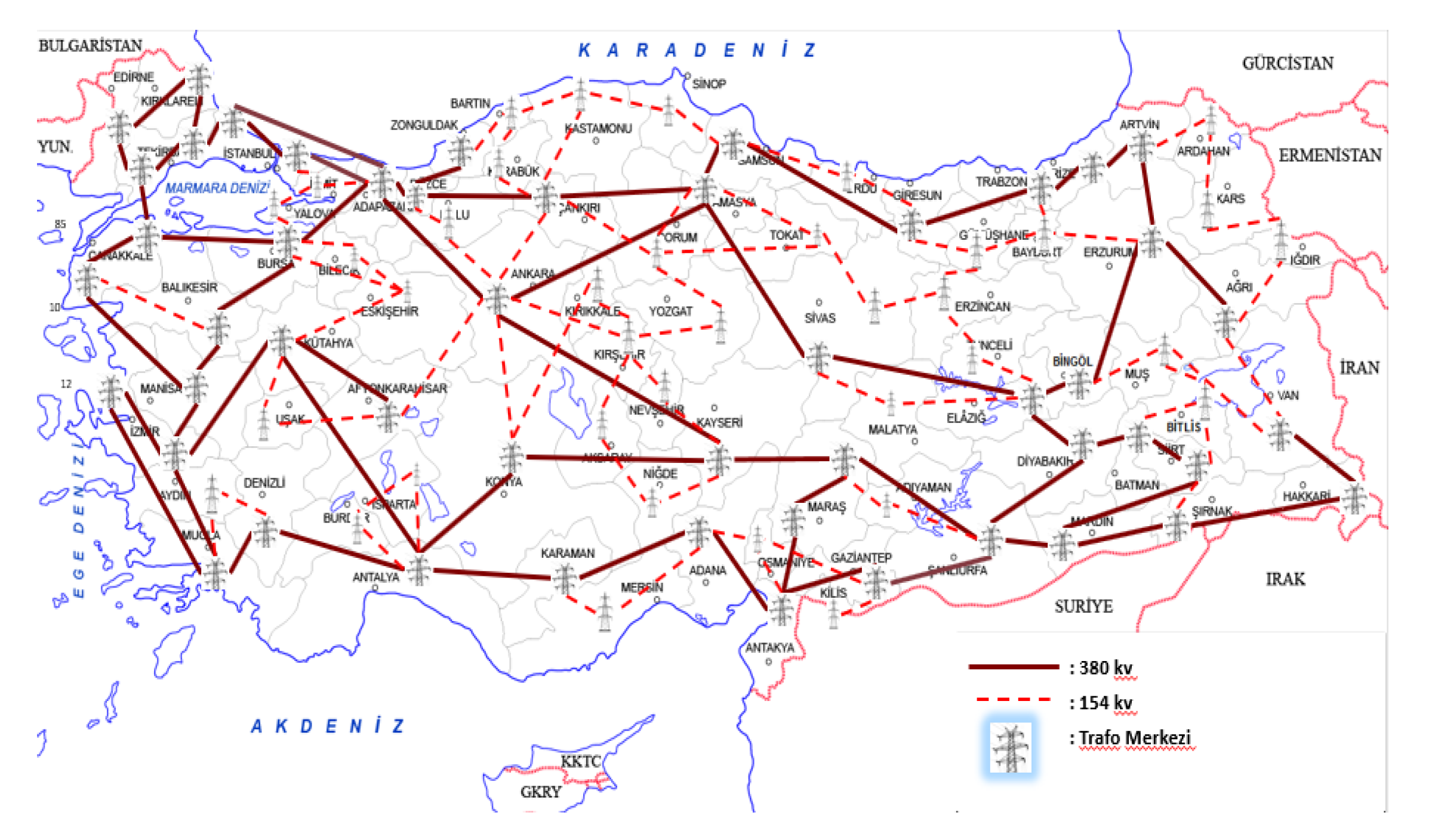
A case study for the Turkish power systems includes 81 pricing nodes, 153 transmission lines, and 318 generators. Eighty-one pricing nodes are selected from 81 cities in Turkey. The transmission network as used in the case study is illustrated in Figure 1. Transmission lines of 154 kV and 380 kV are considered in this study and their electricity carrying capacity is altered according to their size.

The generator dataset aggregates the individual power plants in a city into a single power plant by fuel type. Fifteen fuel types are considered in the study: asphaltite, biogas, coal, fuel oil, geothermal, hydro, import coal, lignite, LPG, naphtha, natural gas, solar plant, thermal plant, waste heat, and wind. A power plant by fuel type is assigned to each city if there is a power plant in the city’s footprint. A fuel cost is assigned to all fuel types. The intermittency of renewable energy, such as wind, solar, and hydro, are assumed to have a scheduled profile for the day. Therefore, no renewable curtailment or dispatchable capacity is assumed. The geographical locations of the generators as adopted in the case study are illustrated by fuel type in Figure 2.

The historical demand of Turkey in 2019 is extracted from the Turkish Market Operator, Exchange Istanbul (EXIST), transparency platform and used to calculate the nodal demand. Nodal demand data is created by considering the population of the cities. The share of the population is used as the share of electricity consumption. A sample day from 2019 is used in the case study. The optimization problem of Model 1 is written by YALMIP [24] and solved by CPLEX in MATLAB.

3. Cluster Validation

Cluster validation seeks to measure the quality of the clustering. The validity measures are divided into three: external, internal, and relative validations [25].

The external validation is used when the class labels of the dataset are already known. Some examples of external clustering validation measures are purity, maximum matching, and F-measure [26]. These measures evaluate all points in the dataset by comparing their pre-label and post-labels. The contingency table induced for each cluster is constructed and all three external measures can be calculated accordingly. However, the clustering of LMPs for an electricity market is an unsupervised learning problem. Hence, there exist no class labels at the beginning of the problem. Therefore, the external validation measures do not apply to such clustering.

The internal validation measures consist of calculations related to the data itself such as intra-cluster and inter-cluster distances [27]. The Silhouette score concept is an internal valuation of the clustering [26]. The silhouette coefficient (SC) of the clustering is defined by Equation (8).

SC = (∑s_i)/n

(8)

where n is the number of points in the dataset and s_i is the silhouette score of each point in the dataset, as given in Equation (9).

$$s_i=\frac{{\mu }_{out}^{min}\left(x_i\right)-{\mu }_{in}\left(x_i\right)}{max\left\{{\mu }_{out}^{min}\left(x_i\right),{\mu }_{in}\left(x_i\right)\right\}}$$

(9)

where $x_i$ is any point in the dataset, ${\mu }_{out}^{min}\left(x_i\right)$ is the mean distances between $x_i$ and points in the closest cluster, and ${\mu }_{in}\left(x_i\right)$ is the mean distance between $x_i$ and points in its own cluster. The silhouette score and silhouette coefficient lie in the interval [−1, 1]. For Equation (9) to be close to 1, ${\mu }_{out}^{min}\left(x_i\right)$ should be greater than ${\mu }_{in}\left(x_i\right)$, as ${\mu }_{in}\left(x_i\right)$ is a measure of how dissimilar $x_i$ is to its own cluster and ${\mu }_{in}\left(x_i\right)$ is a measure of how dissimilar $x_i$ to other clusters. For Equation (9) to be close to −1, however, we require ${\mu }_{in}\left(x_i\right)$ to be greater than ${\mu }_{out}^{min}\left(x_i\right)$, which implies a high dissimilarity within the cluster. Therefore, if the coefficient is close to 1, we can conclude that the resultant clusters are dense and well separated. However, if the coefficient is close to −1, the points are mis-clustered in which the similarity of $x_i$ with other clusters is greater than the similarity with its own cluster.

The relative validation requires varying parameter values, such as the number of clusters to evaluate the quality of the clustering. The elbow method uses a varying number of clusters versus the Within-Cluster-Sum of Squares (WCSS) to calculate the quality of the cluster. The k represents the number of clusters that the user expects to see in this unlabeled data. Therefore, it is a parameter to choose by experience or by some other methods, such as the elbow method. The very first application of the elbow method can be traced back to an article in Psychometrika [28], and it has been used as one of the methods for determining the number of clusters in a data set in different domains, such as electrical engineering [29,30], computer science [31], education [32], statistics [33,34], and communications [35,36].

To find the optimal k value in the k-means clustering algorithm, the elbow method shall be applied to the data. Since the elbow method runs k-means clustering on the dataset for a range of values of k, then, for each k value, it computes the WCSS for all clusters. The WCSS is the sum of the squared distance between each member of the cluster and its centroid is given in Equation (10).

WCSS = ∑ (x_i,j − c_j)²

(10)

where x_i,j is the ith observation assumed to be in Cluster j in the dataset and c_j is the centroid of the Cluster j. For a multi-dimensional space, the centroid is the mean position of all the points in all the coordinate directions. The calculation of WCSS even for a given number of clusters k has a Non-deterministic Polynomial-time (NP) hard complexity [37], but existing heuristic algorithms may converge to a local optimum.

Once the WCSS and the number of clusters are illustrated in a two-dimensional graph, it is likely to have WCSS beginning to level off at a certain number of clusters. The shape of the curve looks like an elbow, where the method takes its name of the elbow method. The elbow method suggests the optimal k-value where the change in WCSS begins to level off.

4. Zone Detection by k-Means Clustering

One of the methods that can be used to determine a pricing zone in the electricity market is the method of the k-means clustering by using the similarity of locational marginal prices. k-means clustering is a highly used, unsupervised clustering algorithm that takes unlabeled data and returns the cluster label of entries out of a k number of clusters. It is originally developed to grouping n observations into k clusters based on the distance of the observation and the center or centroid of the cluster that the observation belongs to [38]. Although there are variations on algorithms applied to different types of datasets, the method has been used in several studies in power systems [39,40,41,42].

In the market, the zone is used as a terminology, as an area formed by price points where electricity prices are similar or the same. For this reason, using the k-means clustering algorithm on the LMPs calculated by Model 1 may open the way for the nodes with similar prices to be placed in the same cluster and to use the nodes in this cluster as a zone. In this study, the k-means clustering algorithm is applied to the LMP results from Model 1 for a 24-h horizon and, thus, group the price points into clusters, including the hourly price changes during the day.

In addition, 24-h LMPs of all nodes are used in the k-means algorithm to detect the pricing zones with similar LMPs. The elbow method is applied to the dataset to find the optimal k value. Figure 3 represents the within-cluster-sum-of-squares (WCSS) versus the number of clusters. The elbow is seen when the number of clusters is three. Since the elbow method is only a decision support mechanism, four clusters are also studied.

A further internal valuation analysis by a silhouette score method to verify the findings of the relative valuation by the elbow method is studied and silhouette scores of each point and clusters (in different colors), as well as the cluster silhouette coefficient (red dashed line), are illustrated in Figure 4 for the k-means algorithm. The silhouette score of three clusters is closer to 1 than the four clusters, indicating a more dense and well-separated clustering.

Figure 5a illustrates the three-means clustering results of the 24-h Locational Marginal Prices (LMP). Four-means clustering results are also illustrated in Figure 5b.

The statistical measures to understand the differences between clusters are given in

Table 1. Statistical measures of k-means clustering.

Method		24-h k-Means Clustering
Number of Clusters		3			4
Cluster Label		0	1	2	0	1	2	3
Min	$/MWh	10.48	37.58	23.34	18.63	25.12	37.58	10.48
25% percentile	$/MWh	16.47	40.29	26.17	19.38	26.59	40.29	16.39
Mean	$/MWh	17.76	40.79	27.74	20.28	28.24	40.8	16.47
Median	$/MWh	17.45	41.57	27.23	20.06	27.93	41.57	16.51
75% percentile	$/MWh	19.45	42.04	29.47	20.66	29.89	42.04	16.94
Max	$/MWh	21.9	42.5	34.14	23.57	34.14	42.5	18.53
Std. Dev.	$/MWh	2.13	1.77	2.59	1.3	2.26	1.77	1.49
Variance	$/MWh	4.57	3.13	6.75	1.69	5.13	3.13	2.23

for 24-h k-mean clustering results. The mean values of LMPs within the clusters are changing from $16.47/MWh to $40.80/MWh when four clusters are generated from a daily dataset.

5. Zone Detection by Spatially Constrained Clustering

Since the k-means clustering method in Section 4 only uses hourly electricity prices as input, the geographical features of these price points are not used when separating the zones. For this reason, while determining zones, the neighborhood status of the cities is not evaluated. In electricity markets where zonal pricing is applied, power transmission flow restrictions between two zones are generally imposed, implying that the zones are geographically as well as electrically separated from each other. When using these power transmission flow constraints, the cities that make up a zone are expected to be neighbors to each other. Therefore, a temporal and spatial clustering method including geographical neighborhood information is required. This method is called spatially constrained clustering. The early applications of spatially constrained clustering are applied to landscape and vegetation [43,44,45]. However, it is now used in various disciplines such as geoinformatics [46], energy modeling [47], and pattern recognition [48].

Generally, in such studies, an assumption must be made of which geographical region the price point represents. A price point can refer to a district, a city, or a region that includes several of them. On behalf of emulating the example in the previous section, this section will also accept every price point as an expression of a city in Turkey. In this case, 81 price points for 81 cities in Turkey and the geographical proximity of the city on the map have been identified. These data are usually kept in GeoJson files.

A similar but slightly different approach than the k-means algorithm is required to satisfy the spatial contiguity condition. The new clustering problem called the max-p-regions problem can be modeled as Mixed-Integer Programming (MIP) and it can be solved by a heuristic approach [49]. There are two different algorithms to which the spatially constrained clustering method can be applied. These are the neighborhood detection algorithms named Queen and Rook, which are referred to as their equivalents in the chess game. If you consider the movement characteristics of the rook in the game of chess, it is necessary to have the border of two cities in the north, south, east, or west in order to understand whether the two cities are neighbors. Similarly, like the full free movement features of the Queen in chess, even if two cities have a border at only one point, this point neighborhood is valued during zone selection. It should not be forgotten that, if a study is conducted over smaller settlements rather than cities, as in our example, the two methods may yield completely different results. Nevertheless, in our example here, some cities have a point neighborhood, and, therefore, the zone detection has been completed with both Queen and Rook algorithms.

In the Queen and Rook algorithms, where evaluated within the clustering method in geographical neighborhoods, a threshold value is determined depending on the value of the parameter to be clustered (it is the hourly price for the electricity market). This value is one of the inputs of the algorithms. Depending on this threshold value, the algorithms utilize a heuristic method to minimize the number of clusters while placing neighboring points within the threshold into the same cluster [50]. While creating these zones, cluster numbers were not given to the algorithms as in Section 4, but the desired number of zones was obtained by changing the threshold value. In Figure 6a,c, pricing zones created with Queen neighborhood features are shown with a threshold value of 0.2 and 0.15, respectively. Similarly, the electrical pricing zones determined by Rook neighborhood features are shown in Figure 6b,d with a threshold value of 0.2 and 0.14, respectively.

For a quantitative comparison of queen and rook algorithms within the framework of spatially constrained clustering (SCC), the statistical measures are given in

Table 2. Statistical measures of queen-based spatially constrained clustering.

Method		Queen-Based Spatially Constrained Clustering
Number of Clusters		3			4
Cluster Label		0	1	2	0	1	2	3
Min	$/MWh	12.35	10.49	18.08	10.49	12.35	16.42	16.29
25% percentile	$/MWh	16.52	16.47	21.16	16.48	16.47	18.64	18.64
Mean	$/MWh	19.58	19.85	25.36	21.41	19.38	21.47	25.38
Median	$/MWh	17.82	16.84	25.85	19.29	16.76	20.30	25.70
75% percentile	$/MWh	19.38	19.30	27.76	22.88	19.50	25.13	28.92
Max	$/MWh	42.04	42.50	41.58	40.29	42.50	27.93	42.04
Std. Dev.	$/MWh	6.11	7.58	4.88	7.18	6.43	3.68	8.00
Variance	$/MWh	37.35	57.47	23.84	51.55	41.38	13.57	63.94

for queen-based SCC and

Table 3. Statistical measures of rook-based spatially constrained clustering.

Method		Rook-Based Spatially Constrained Clustering
Number of Clusters		3			4
Cluster Label		0	1	2	0	1	2	3
Min	$/MWh	10.49	13.98	18.08	10.49	12.35	18.08	16.29
25% percentile	$/MWh	16.47	16.49	21.91	16.48	16.46	22.92	16.64
Mean	$/MWh	20.36	19.16	26.65	19.62	20.63	26.14	21.05
Median	$/MWh	19.12	16.92	26.59	18.15	16.97	26.48	19.01
75% percentile	$/MWh	20.39	19.01	28.79	20.31	19.64	27.41	21.24
Max	$/MWh	40.29	42.50	42.04	40.29	42.50	41.58	42.04
Std. Dev.	$/MWh	6.48	5.81	6.06	5.73	8.02	5.29	6.28
Variance	$/MWh	42.01	33.77	36.72	32.86	64.37	27.97	39.46

for rook-based SCC.

For comparison of different clustering methods used to determine pricing zones in this study, the silhouette coefficients are given in

Table 4. Silhouette coefficients of clustering methods.

Method	Number of Clusters	Silhouette Coefficient
k-means clustering	3	0.730
k-means clustering	4	0.576
Queen-based SCC	3	−0.019
Queen-based SCC	4	−0.101
Rook-based SCC	3	0.015
Rook-based SCC	4	−0.084

. The k-clustering method using three zones resulted in the most dense and well-separated clusters, while the Queen-based SCC with four zones had the least.

6. Discussion

6.1. Economic Impact

While electrical energy is bought and sold as a commodity under market conditions, the price formed as an output of this market must be formed correctly. Commodity prices are an argument used as a signal in investor decisions. Thanks to this signal, investors can make the right decisions from choice of location to capacity selection in their buy or sell investments.

The method that can be used in the transition to zonal pricing in the national markets, where a single price is used in the electricity market, is explained in this study. In the later stages of the study, we plan to examine the differences that may occur according to the use of the created zones within a market structure and the single price market structure. At the same time, we want to analyze the impact of zonal pricing on the intraday market with combined modeling as day-ahead and intraday markets in the market design phase.

Uniform marginal price application, which is used as pricing of electrical energy regardless of location, eliminates the feature of location choice in investment decisions and signals that the investment can be made anywhere in the country. However, regional pricing can create an accurate signal for investors in their decisions due to the energy losses that occur between the places where electrical energy is produced and consumed and the congestion that may occur during electricity transmission. Changing zonal prices may reveal that there is no balance between supply and demand within a zone. Therefore, it is necessary to purchase electricity from another zone or to transmit electricity to another zone. It is understood that demand is higher than supply in zones where electricity prices are higher, and this price signal encourages investors to put generation plants in this region. Similarly, in zones with lower prices, it is understood that supply is higher than demand and investors increase the demand in that region by increasing their industrial investments in regions where cheaper electricity can be purchased. Considering the regional pricing practice only as a method in which prices differ is a deficiency at this point. In fact, zonal pricing is an application that affects investment decisions and serves as a signal for the formation of the supply-demand balance.

6.2. Social and Political Impact

The price of electricity is a social measure that has a big impact not only in the energy sector but anywhere electricity is consumed. The price might also be used as a political instrument by policymakers. The pricing system of electricity is not only related to engineering and mathematical modeling disciplines. It is a very important commodity of society that should be discussed in a multi-disciplinary platform. From an engineering perspective, the proposed methodology of electricity pricing based on an optimization problem to minimize the total production cost of electricity (Model 1) is intended to maximize social welfare. Further explanations on the zonal markets and also the discussions around how to find the best pricing zones in this study may not capture and assess the political background of the energy sector entirely. However, the intentions of mathematical modeling with the support of various simulations are always the beginning of multi-disciplinary studies to quantify the necessity of a bigger change in society. The planned future work of this study is further discussed in Section 6.3.

6.3. Future Work

The method that can be used in the transition to zonal pricing in the national markets, where a single price is used in the electricity market, is explained in this study. In future work, we plan to examine the differences that may occur in the bidding structure of the power market, according to the use of the proposed zones. At the same time, we want to analyze the impact of zonal pricing on the intraday market with combined modeling as day-ahead and intraday markets as well as the balancing mechanism prices in the market design phase.

7. Conclusions

Day-ahead electricity markets are an auction-based market where supply and demand are brought together. Considering the physical properties of electrical energy, it can be modeled as an optimization problem to maximize social welfare. While designing a national electricity market, which is generally built on creating a single national price in the first place, deepen with the transition to zonal or locational pricing methods and create a more competitive structure.

This paper describes three clustering methods that might be used in zone detection for a power market in the transition from a uniform price to a zonal price mechanism in the day-ahead electricity market. For a case study of Turkey, three algorithms are tested, and the final clusters’ geographical representations are illustrated on a map. These methods can be used by policy-makers as a decision support mechanism. By optimal power flow model as given in Model 1, locational marginal prices can be calculated for each price point. Then zones can be determined by combining points with similar price ranges. One of the methods described in this article is the spatial constraint clustering method, which works to include the geographical proximity of price points, instead of single clustering by LMPs. In this method, different zone preferences can be made by determining neighborly relations as queen and rook, and different zone preferences can be formed by changing the geographical regions expressed by point prices.