
Optimal Scheduling of Non-Convex Cogeneration Units Using Exponentially Varying Whale Optimization Algorithm

 ,
,  ,
,  , , and
Abstract
1. Introduction
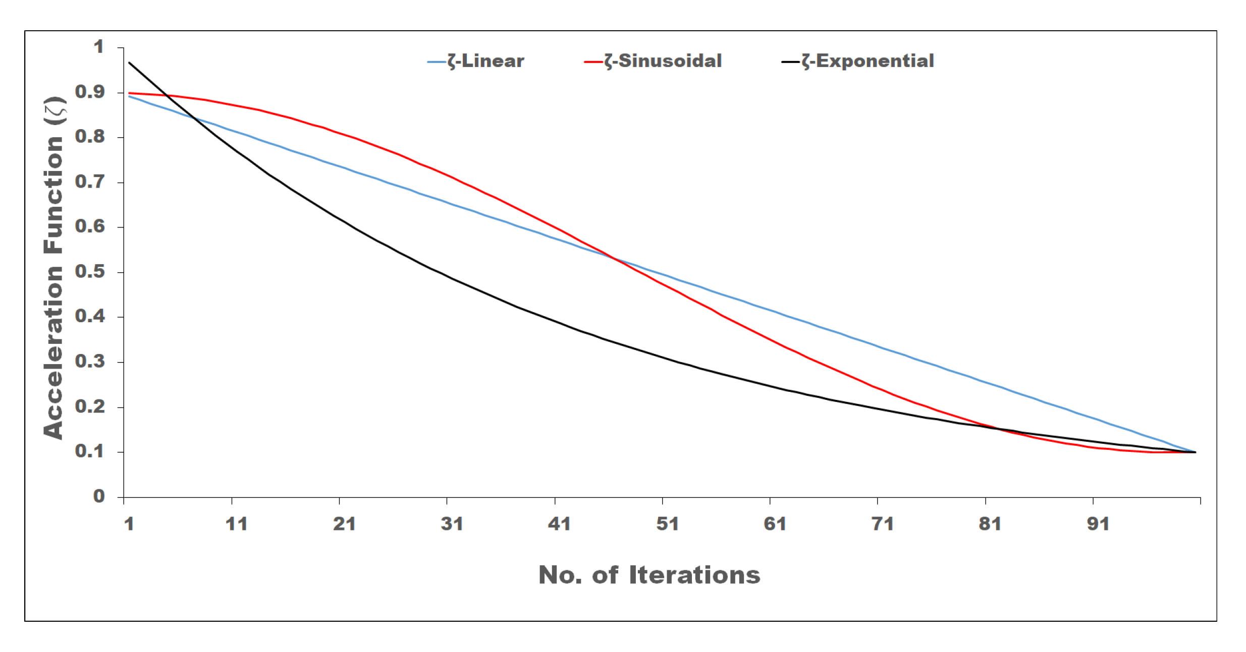
- Four different variants of WOA are considered for improving and enhancing the performance of the basic WOA. In the first variant of WOA, the acceleration function is randomly selected, and it is written as Randomly Varying WOA (RVWOA). In the second variant of WOA, the acceleration function is linearly varied and is called Linearly Varying WOA (LVWOA), the third variant is Sinusoidally Varying WOA (SVWOA), where the acceleration function is varied Sinusoidally. In addition, in the proposed variant, Exponentially Varying WOA (EVWOA), the exponentially varied acceleration function is used.
- All the four variants of WOA and basic WOA are tested on well-known and standard benchmark functions for performance evaluation and later on six small to large different CHP case studies.
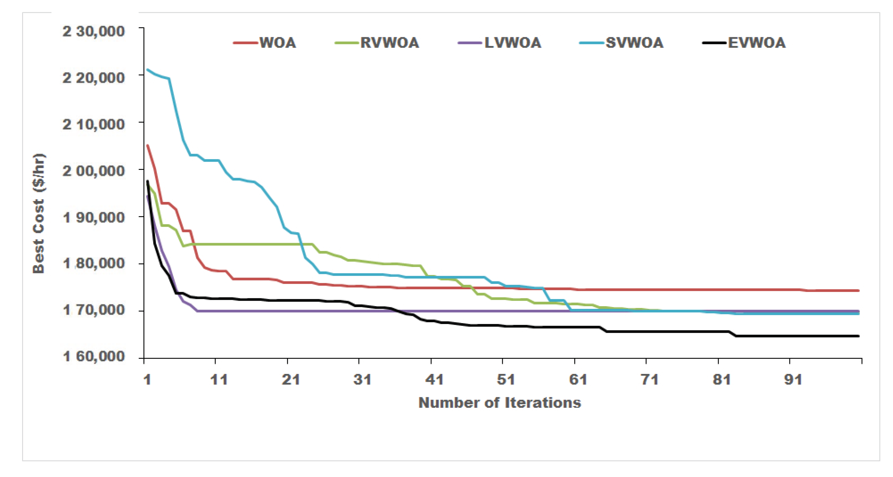
- Simulation results generated by EVWOA after independent 100 different trials are compared with basic WOA, other remaining variants of WOA, and recently published results obtained by different latest methods. The comparison results show that the proposed EVWOA performs much better than other latest methods.
2. Problem Formulation
2.1. Constraints
2.1.1. Equality Constraints
2.1.2. Inequality Constraints
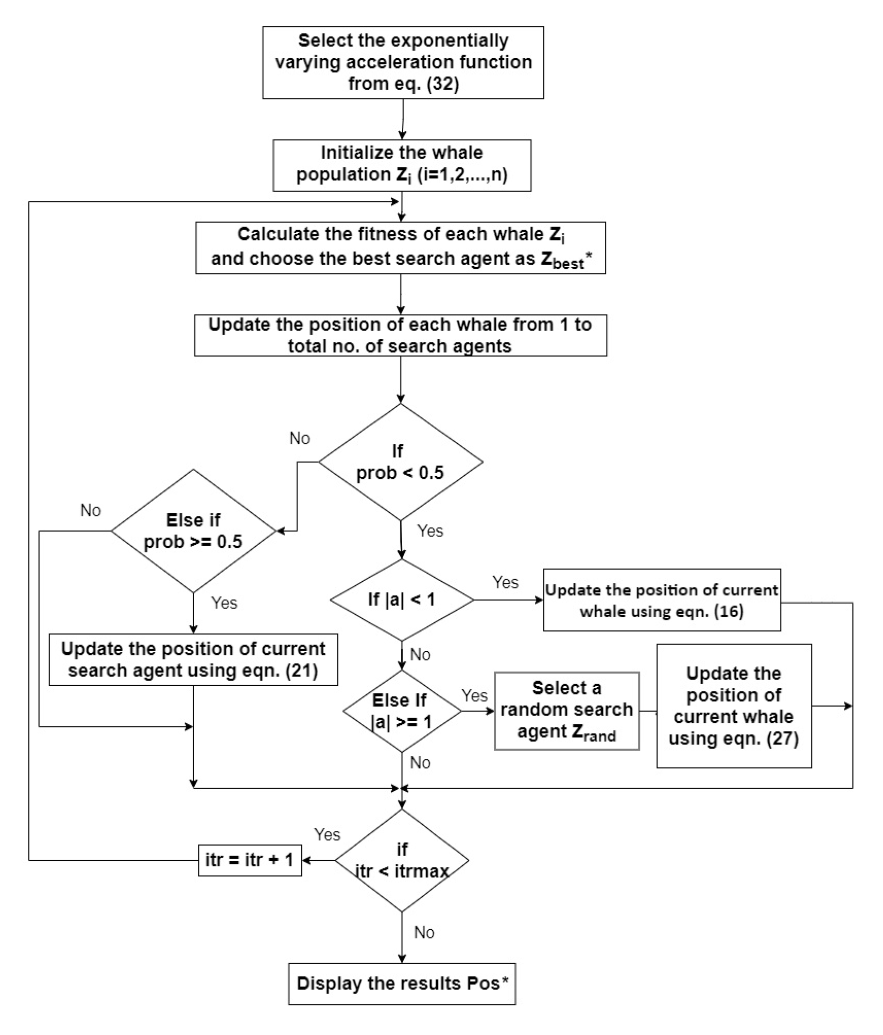
3. Proposed Exponentially Varying Whale Optimization Algorithm (EVWOA)
3.1. Encircling Prey
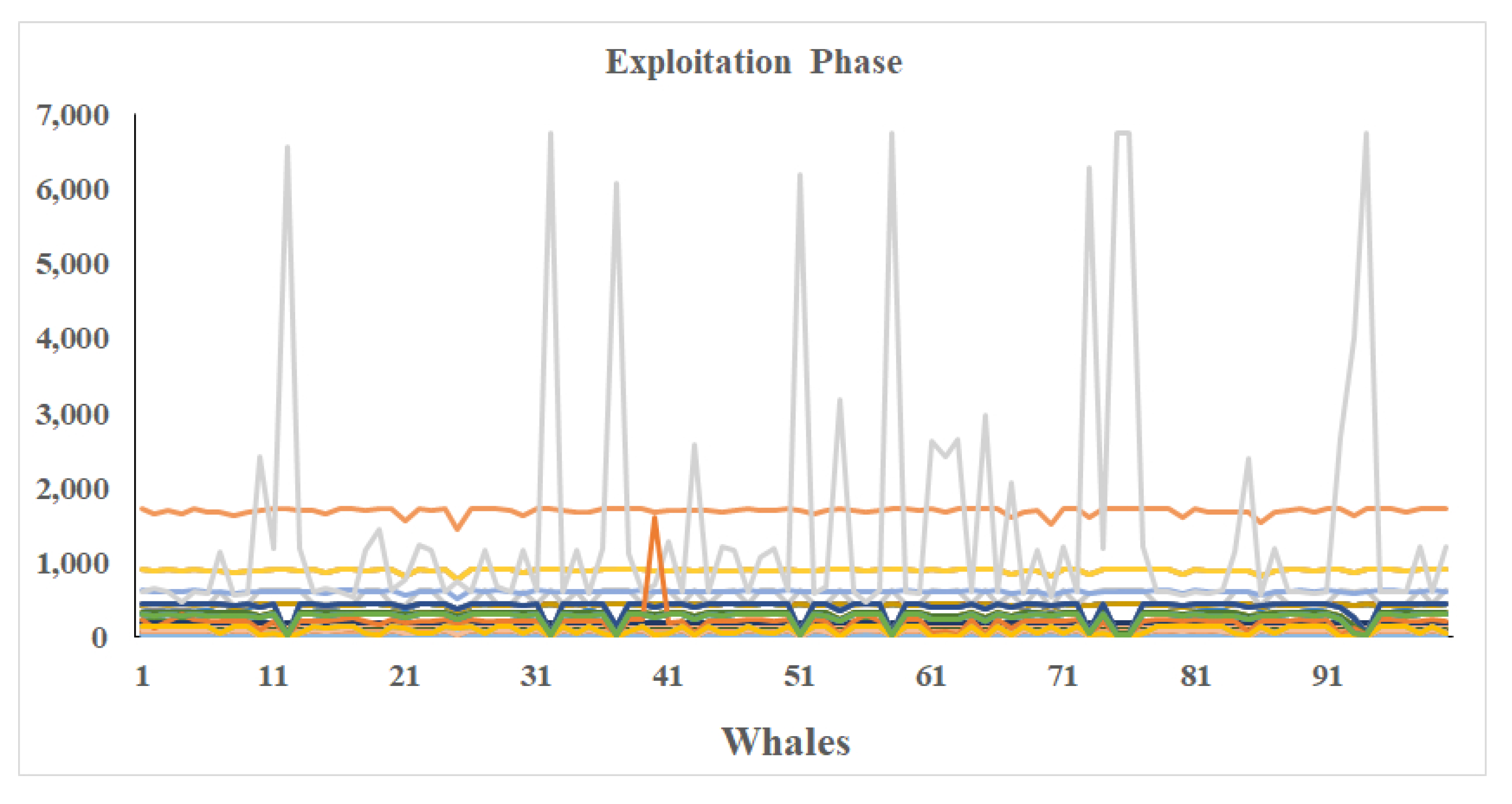
3.2. Exploitation Phase
3.2.1. Shrinking Encircling
3.2.2. Spiral Updating Position
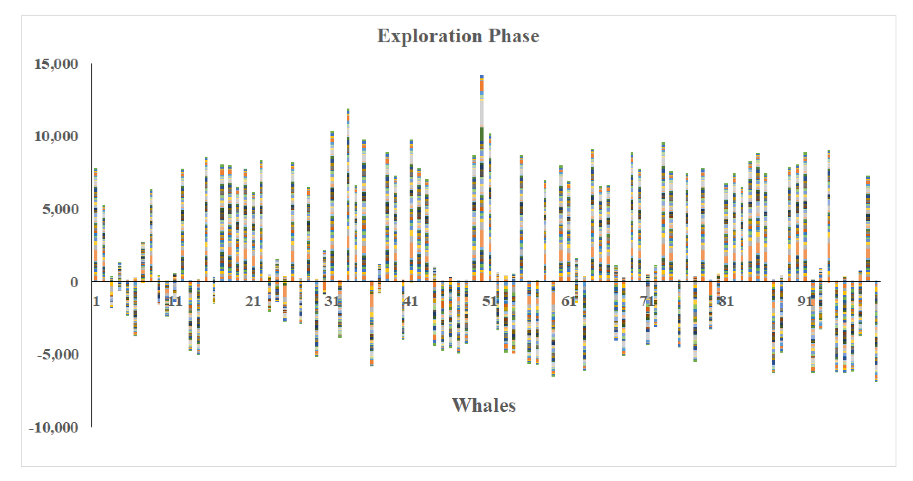
3.3. Exploration Phase
3.4. Choice of Acceleration Function
- Randomly Varying WOA (RVWOA)
- Linearly Varying WOA (LVWOA)
- Sinusoidally Varying WOA (SVWOA)
- Exponentially Varying WOA (EVWOA)
- Randomly Varying WOA (RVWOA): In the first variant of WOA, acceleration function is randomly selected between [0,1] as in Reference [29].
- Sinusoidally Varying WOA (SVWOA): In this variant, the acceleration function () is varied sinusoidally from 0.9 to 0.1 as in [39]. The mathematical expression is given below:where = X * itr + Y and the coefficients X and Y are calculated by Equations (30) and (31) and iteration (itr) is varied from itrmin to itrmax.
- Exponentially Varying WOA (EVWOA): In this proposed variant, the acceleration function () is varied exponentially as in [40]. The exponential variation of is calculated by the following relation:where and is the ratio of maximum minimum bounds of the acceleration function.
3.5. Testing of the WOA Variants on Well-Known Benchmark Functions
4. Results and Discussions
4.1. Case Study 1
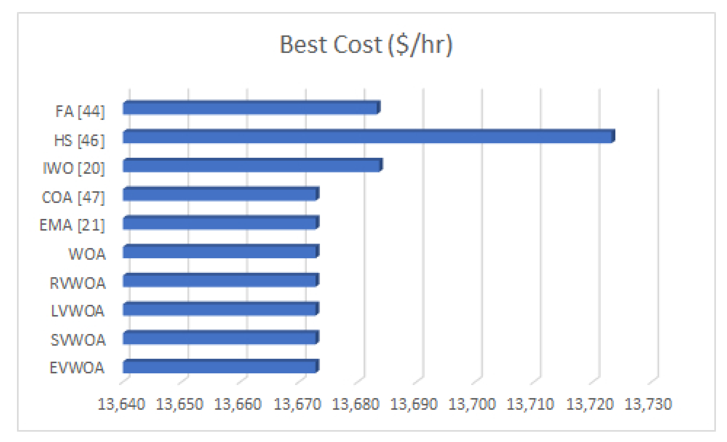
4.2. Case Study 2
4.3. Case Study 3
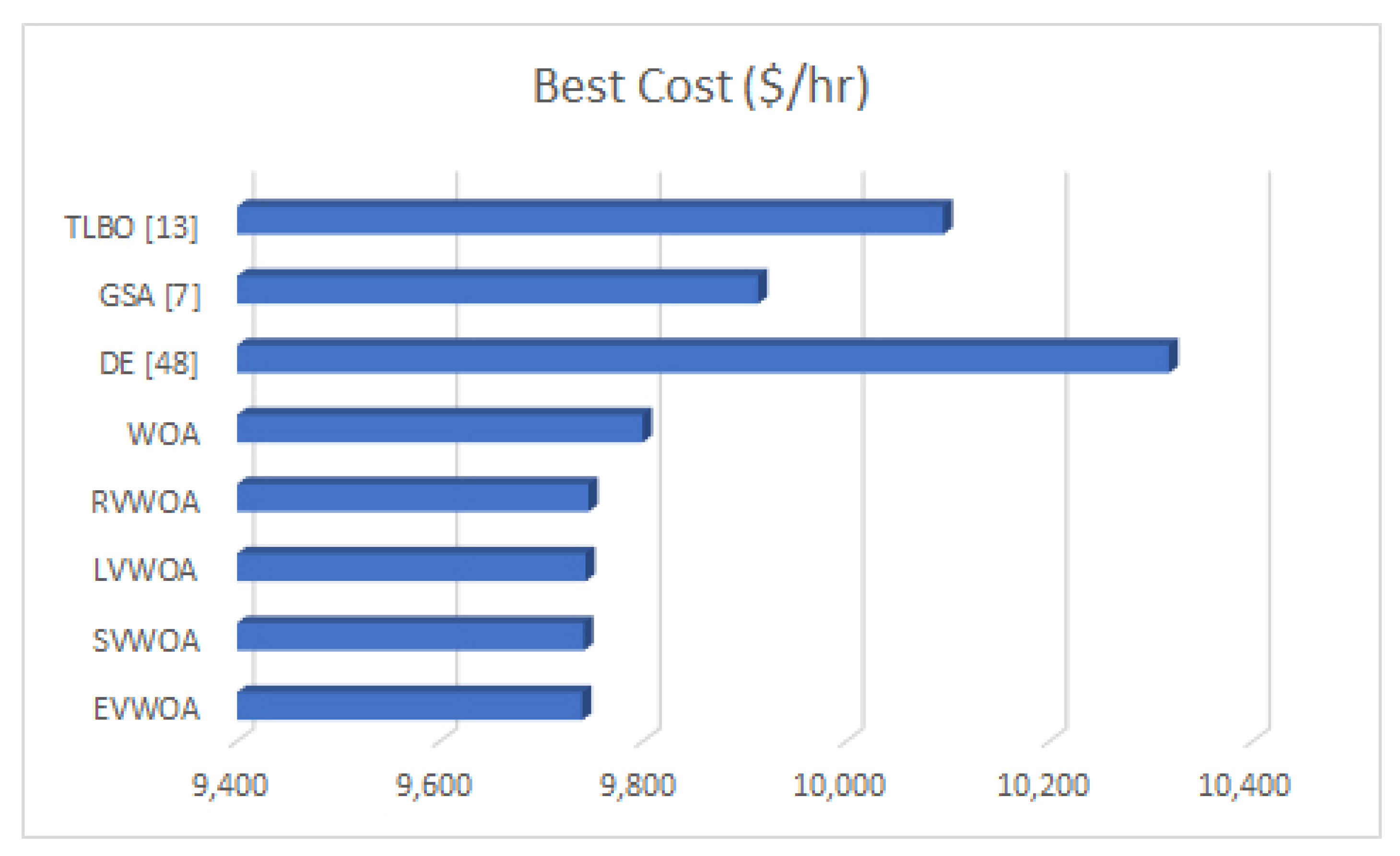
4.4. Case Study 4
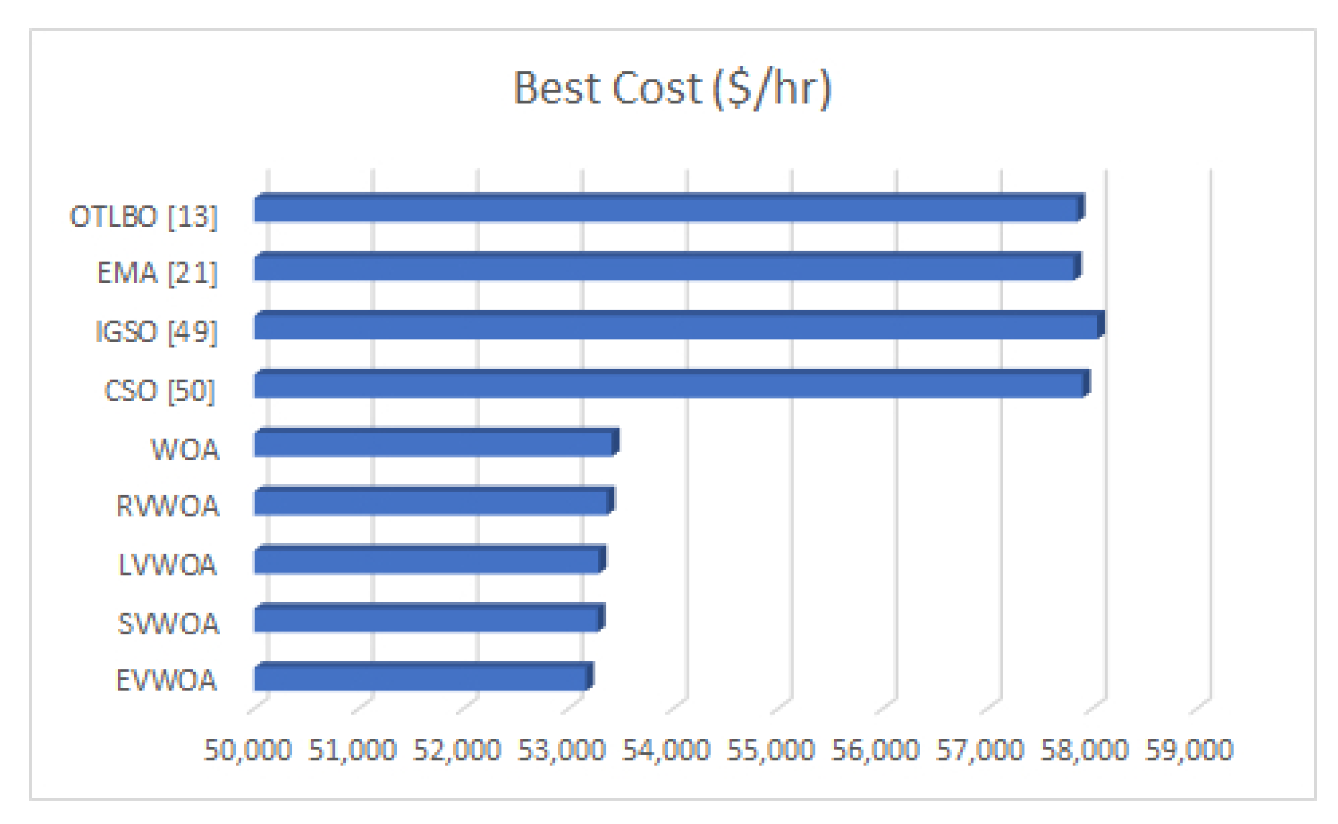
4.5. Case Study 5
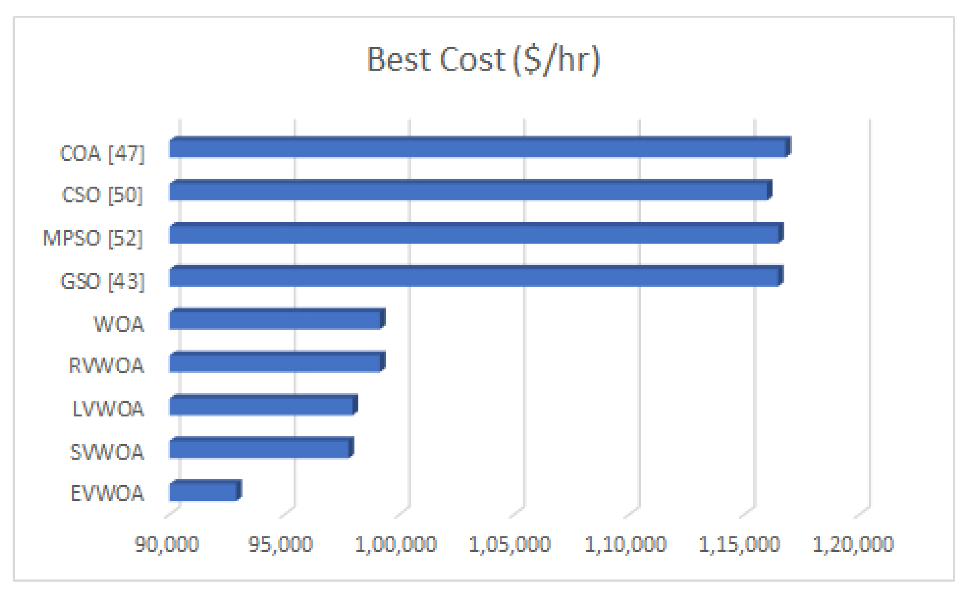
4.6. Case Study 6
Discussion about Convergence Characteristics
5. Conclusions
Author Contributions
Funding
Institutional Review Board Statement
Informed Consent Statement
Conflicts of Interest
Appendix A

| Unit | a ($/MW2) | b ($/MW) | c ($) | Pmin (MW) | Pmax (MW) |
|---|---|---|---|---|---|
| 1 | 0 | 50 | 0 | 0 | 150 |
| Unit | a ($/MW2) | b ($/MW) | c ($) | d ($/MWth2) | e ($/MWth) | f ($/MW.MWth) | FOR (P,H) |
|---|---|---|---|---|---|---|---|
| 2 | 0.0345 | 14.5 | 2650 | 0.030 | 1.200 | 0.031 | [98.8, 0], [81, 104.8], [215, 180], [247, 0] |
| 3 | 0.0435 | 36.0 | 1250 | 0.027 | 0.600 | 0.011 | [44, 0], [44, 15.9], [40, 75], [110.2, 135.6], [125.8, 32.4], [125.8, 0] |
| Unit | a ($/MW2) | b ($/MW) | c ($) | Hmin (MWth) | Hmax (MWth) |
|---|---|---|---|---|---|
| 4 | 0 | 23.4 | 0 | 0 | 2695.2 |
Appendix B
| Unit | h ($/MW3) | a ($/MW2) | b ($/MW) | c ($) | Pmin (MW) | Pmax (MW) |
|---|---|---|---|---|---|---|
| 1 | 0.000115 | 0.00172 | 7.6997 | 254.8863 | 0 | 35 |
| Unit | a ($/MW2) | b ($/MW) | c ($) | d ($/MWth2) | e ($/MWth) | f ($/MW.MWth) | FOR (P,H) |
|---|---|---|---|---|---|---|---|
| 2 | 0.0435 | 36.0 | 1250 | 0.027 | 0.600 | 0.011 | [44, 0], [44, 15.9], [40, 75], [110.2, 135.6], [125.8, 32.4], [125.8, 0] |
| 3 | 0.1035 | 34.5 | 2650 | 0.025 | 2.203 | 0.051 | [20, 0], [10, 40], [45, 55], [60, 0] |
| 4 | 0.072 | 20 | 1565 | 0.02 | 2.340 | 0.04 | [35, 0], [35, 20], [90, 45], [90, 25], [105, 0] |
| Unit | a ($/MW2) | b ($/MW) | c ($) | Hmin (MWth) | Hmax (MWth) |
|---|---|---|---|---|---|
| 5 | 0.038 | 2.0109 | 950 | 0 | 60 |
Appendix C
| Unit | a ($/MW2) | b ($/MW) | c ($) | d ($) | e (rad/MW) | Pmin (MW) | Pmax (MW) |
|---|---|---|---|---|---|---|---|
| 1 | 0.008 | 2 | 25 | 100 | 0.042 | 10 | 75 |
| 2 | 0.003 | 1.8 | 10 | 140 | 0.04 | 20 | 125 |
| 3 | 0.0012 | 2.1 | 100 | 160 | 0.038 | 30 | 175 |
| 4 | 0.001 | 2 | 120 | 180 | 0.037 | 40 | 250 |
| Unit | a ($/MW2) | b ($/MW) | c ($) | d ($/MWth2) | e ($/MWth) | f ($/MW.MWth) | FOR (P,H) |
|---|---|---|---|---|---|---|---|
| 5 | 0.0345 | 14.5 | 2650 | 0.030 | 1.200 | 0.031 | [98.8, 0], [81, 104.8], [215, 180], [247, 0] |
| 6 | 0.0435 | 36.0 | 1250 | 0.027 | 0.600 | 0.011 | [44, 0], [44, 15.9], [40, 75], [110.2, 135.6], [125.8, 32.4], [125.8, 0] |
| Unit | a ($/MW2) | b ($/MW) | c ($) | Hmin (MWth) | Hmax (MWth) |
|---|---|---|---|---|---|
| 7 | 0.038 | 2.0109 | 950 | 0 | 2695.2 |
Appendix D
| Unit | a ($/MW2) | b ($/MW) | c ($) | d ($) | e (rad/MW) | Pmin (MW) | Pmax (MW) |
|---|---|---|---|---|---|---|---|
| 1 | 0.00028 | 8.1 | 550 | 300 | 0.035 | 0 | 680 |
| 2,3 | 0.00056 | 8.1 | 309 | 200 | 0.042 | 0 | 360 |
| 4,5,6,7,8,9 | 0.00324 | 7.74 | 240 | 150 | 0.063 | 60 | 180 |
| 10,11 | 0.00284 | 8.6 | 126 | 100 | 0.084 | 40 | 120 |
| 12,13 | 0.00284 | 8.6 | 126 | 100 | 0.084 | 55 | 120 |
| Unit | a ($/MW2) | b ($/MW) | c ($) | d ($/MWth2) | e ($/MWth) | f ($/MW.MWth) | FOR (P,H) |
|---|---|---|---|---|---|---|---|
| 14,16 | 0.0345 | 14.5 | 2650 | 0.030 | 1.200 | 0.031 | [98.8, 0], [81, 104.8], [215, 180], [247, 0] |
| 15,17 | 0.0435 | 36.0 | 1250 | 0.027 | 0.600 | 0.011 | [44, 0], [44, 15.9], [40, 75], [110.2, 135.6], [125.8, 32.4], [125.8, 0] |
| 18 | 0.1035 | 34.5 | 2650 | 0.025 | 2.203 | 0.051 | [20, 0], [10, 40], [45, 55], [60, 0] |
| 19 | 0.072 | 20 | 1565 | 0.02 | 2.340 | 0.04 | [35, 0], [35, 20], [90, 45], [90, 25], [105, 0] |
| Unit | a ($/MW2) | b ($/MW) | c ($) | Hmin (MWth) | Hmax (MWth) |
|---|---|---|---|---|---|
| 20 | 0.038 | 2.0109 | 950 | 0 | 2695.2 |
| 21,22 | 0.038 | 2.0109 | 950 | 0 | 60 |
| 23,24 | 0.052 | 3.0651 | 480 | 0 | 120 |
Appendix E
| Unit | a ($/MW2) | b ($/MW) | c ($) | d ($) | e (rad/MW) | Pmin (MW) | Pmax (MW) |
|---|---|---|---|---|---|---|---|
| 1,14 | 0.00028 | 8.1 | 550 | 300 | 0.035 | 0 | 680 |
| 2,3,15,16 | 0.00056 | 8.1 | 309 | 200 | 0.042 | 0 | 360 |
| 4,5,6,7,8,9, 17,18,19,20, 21,22 | 0.00324 | 7.74 | 240 | 150 | 0.063 | 60 | 180 |
| 10,11,23,24 | 0.00284 | 8.6 | 126 | 100 | 0.084 | 40 | 120 |
| 12,13,25,26 | 0.00284 | 8.6 | 126 | 100 | 0.084 | 55 | 120 |
| Unit | a ($/MW2) | b ($/MW) | c ($) | d ($/MWth2) | e ($/MWth) | f ($/MW.MWth) | FOR (P,H) |
|---|---|---|---|---|---|---|---|
| 27,29, 33,35 | 0.0345 | 14.5 | 2650 | 0.030 | 1.200 | 0.031 | [98.8, 0], [81, 104.8], [215, 180], [247, 0] |
| 28,30, 34,36 | 0.0435 | 36.0 | 1250 | 0.027 | 0.600 | 0.011 | [44, 0], [44, 15.9], [40, 75], [110.2, 135.6], [125.8, 32.4], [125.8, 0] |
| 31,37 | 0.1035 | 34.5 | 2650 | 0.025 | 2.203 | 0.051 | [20, 0], [10, 40], [45, 55], [60, 0] |
| 32,38 | 0.072 | 20 | 1565 | 0.02 | 2.340 | 0.04 | [35, 0], [35, 20], [90, 45], [90, 25], [105, 0] |
| Unit | a ($/MW2) | b ($/MW) | c ($) | Hmin (MWth) | Hmax (MWth) |
|---|---|---|---|---|---|
| 39,44 | 0.038 | 2.0109 | 950 | 0 | 2695.2 |
| 40,41,45,46 | 0.038 | 2.0109 | 950 | 0 | 60 |
| 42,43,47,48 | 0.052 | 3.0651 | 480 | 0 | 120 |
Appendix F
| Unit | a ($/MW2) | b ($/MW) | c ($) | d ($) | e (rad/MW) | Pmin (MW) | Pmax (MW) |
|---|---|---|---|---|---|---|---|
| 1,14,27,40 | 0.00028 | 8.1 | 550 | 300 | 0.035 | 0 | 680 |
| 2,3,15,16, 28,29,41,42 | 0.00056 | 8.1 | 309 | 200 | 0.042 | 0 | 360 |
| 4,5,6,7,8,9, 17,18,19,20, 21,22,30,31, 32,33,34,35, 43,44,45,46, 47,48 | 0.00324 | 7.74 | 240 | 150 | 0.063 | 60 | 180 |
| 10,11,23,24, 36,37,49,50 | 0.00284 | 8.6 | 126 | 100 | 0.084 | 40 | 120 |
| 12,13,25,26, 38,39,51,52 | 0.00284 | 8.6 | 126 | 100 | 0.084 | 55 | 120 |
| Unit | a ($/MW2) | b ($/MW) | c ($) | d ($/MWth2) | e ($/MWth) | f ($MW.MWth) | FOR (P,H) |
|---|---|---|---|---|---|---|---|
| 27,29, 33,35 | 0.0345 | 14.5 | 2650 | 0.030 | 1.200 | 0.031 | [98.8, 0], [81, 104.8], [215, 180], [247, 0] |
| 28,30, 34,36 | 0.0435 | 36.0 | 1250 | 0.027 | 0.600 | 0.011 | [44, 0], [44, 15.9], [40, 75], [110.2, 135.6], [125.8, 32.4], [125.8, 0] |
| 31,37 | 0.1035 | 34.5 | 2650 | 0.025 | 2.203 | 0.051 | [20, 0], [10, 40], [45, 55], [60, 0] |
| 32,38 | 0.072 | 20 | 1565 | 0.02 | 2.340 | 0.04 | [35, 0], [35, 20], [90, 45], [90, 25], [105, 0] |
| Unit | a ($/MW2) | b ($/MW) | c ($) | Hmin (MWth) | Hmax (MWth) |
|---|---|---|---|---|---|
| 39,44 | 0.038 | 2.0109 | 950 | 0 | 2695.2 |
| 40,41,45,46 | 0.038 | 2.0109 | 950 | 0 | 60 |
| 42,43,47,48 | 0.052 | 3.0651 | 480 | 0 | 120 |
References
- Keirstead, J.; Samsatli, N.; Shah, N.; Weber, C. The impact of CHP (combined heat and power) planning restrictions on the efficiency of urban energy systems. Energy 2012, 41, 93–103. [Google Scholar] [CrossRef]
- Karki, S.; Kulkarni, M.; Mann, M.D.; Salehfar, H. TEfficiency improvements through combined heat and power for on-site distributed generation technologies. Cogenerat. Distrib. Generat. J. 2007, 3, 19–34. [Google Scholar] [CrossRef]
- Guo, T.; Henwood, M.I.; Ooijen, M.V. An algorithm for combined heat and power economic dispatch. IEEE Trans. Power Syst 1996, 11, 1778–1784. [Google Scholar] [CrossRef]
- Rooijers, F.J.; VanAmerongen, R.A.M. Static economic dispatch for co-generation systems. IEEE Trans. Power Syst 1994, 9, 1392–1398. [Google Scholar]
- Abdol Mohammadi, H.R.; Kazemi, A. A Benders decomposition approach for a combined heat and power economic dispatch. Energy Convers. Manag. 2013, 71, 21–31. [Google Scholar] [CrossRef]
- Song, Y.; Chou, C.; Stonham, T. Combined heat and power economic dispatch by improved ant colony search algorithm. Electric Power Syst. Res. 1999, 52, 115–121. [Google Scholar] [CrossRef]
- Beigvand, S.D.; Abdi, H.; La Scala, M. Combined heat and power economic dispatch problem using gravitational search algorithm. Electric Power Syst. Res. 2016, 133, 160–172. [Google Scholar] [CrossRef]
- Adhvaryyu, P.K.; Chattopadhyay, P.K.; Bhattacharjya, A. Application of bio-inspired krill herd algorithm to combined heat and power economic dispatch. In Proceedings of the 2014 IEEE Innovative Smart Grid Technologies-Asia (ISGTASIA), Kuala Lumpur, Malaysia, 20–23 May 2014; Volume 1, pp. 338–343. [Google Scholar]
- Mohammadi-Ivatloo, B.; Moradi-Dalvand, M.; Rabiee, A. Combined heat and power economic dispatch problem solution using particle swarm optimization with time varying acceleration coefficients. Electr. Power Sys. Res. 2013, 95, 9–18. [Google Scholar] [CrossRef]
- Ramesh, V.; Jayabarathi, T.; Shrivastava, N.; Baska, A. A novel selective particle swarm optimization approach for combined heat and power economic dispatch. Electr. Power Syst. Res. 2009, 37, 1231–1240. [Google Scholar] [CrossRef]
- Subbaraj, P.; Rengaraj, R.; Salivahanan, S. Enhancement of combined heat and power economic dispatch using self-adaptive real-coded genetic algorithm. Appl. Energy 2009, 86, 915–921. [Google Scholar] [CrossRef]
- Khorram, E.; Jaberipour, M. Harmony search algorithm for solving combined heat and power economic dispatch problems. Energy Convers. Manag. 2011, 52, 1550–1554. [Google Scholar] [CrossRef]
- Roy, P.K.; Paul, C.; Sultana, S. Oppositional teaching learning-based optimization approach for combined heat and power dispatch. Int. J. Electr. Power Energy Syst. 2014, 57, 392–403. [Google Scholar] [CrossRef]
- Civicioglu, P.; Besdok, E. TA conceptual comparison of the Cuckoo-search, particle swarm optimization, differential evolution and artificial bee colony algorithms. Artif. Intell. Rev. 2013, 39, 315–346. [Google Scholar] [CrossRef]
- Jena, C.; Basu, M.; Panigrahi, C. Differential evolution with Gaussian mutation for combined heat and power economic dispatch. Soft Comput. 2016, 20, 681–688. [Google Scholar] [CrossRef]
- He, S.; Wu, Q.H. Saunders, J. Group search optimizer: An optimization algorithm inspired by animal searching behaviour. IEEE Trans. Evolut. Comput. 2009, 13, 973–990. [Google Scholar]
- Basu, M. Combined heat and power economic dispatch using opposition-based group search optimization. Int. J. Electr. Power Energy Syst. 2015, 73, 819–829. [Google Scholar] [CrossRef]
- Nguyen, T.T.; Vo, D.N.; Dinh, B.H. Cuckoo search algorithm for combined heat and power economic dispatch. Int. J. Electr. Power Energy Syst. 2016, 81, 204–214. [Google Scholar] [CrossRef]
- Basu, M. Bee colony optimization for combined heat and power economic dispatch. Expert. Syst. Appl. 2011, 38, 13527–13531. [Google Scholar] [CrossRef]
- Jayabarathi, T.; Yazdani, A.; Ramesh, V.; Raghunathan, T. Combined heat and power economic dispatch problem using the invasive weed optimization algorithm. Front. Energy 2014, 8, 25–30. [Google Scholar] [CrossRef]
- Ghorbani, N. Combined heat and power economic dispatch using exchange market algorithm. Int. J. Electr. Power Energy Syst. 2016, 82, 58–66. [Google Scholar] [CrossRef]
- Jayakumar, N. Combined heat and power dispatch by grey wolf optimization. Int. J. Energy Sect. Manag. 2015, 9, 523–546. [Google Scholar] [CrossRef]
- Seyedali, M.; Andrew, L. The Whale Optimization Algorithm. Adv. Eng. Softw. 2016, 95, 51–67. [Google Scholar]
- Nazari-Heris, M.; Mehdinejad, M.; Mohammadi-Ivatloo, B.; Babamalek-Gharehpetian, G. Combined heat and power economic dispatch problem solution by implementation of whale optimization method. Neural Comput. Appl. 2019, 31, 421–436. [Google Scholar] [CrossRef]
- Ying, L.; Yongquan, Z.; Qifang, L. Levy, Flight Trajectory-Based Whale Optimization Algorithm for Global Optimization. IEEE Access. 2017, 5, 6168–6186. [Google Scholar]
- Gaganpreet, K.; Sankalap, A. Chaotic whale optimization algorithm. J. Computat. Des. Eng. 2018, 5, 275–284. [Google Scholar]
- Guojiang, X.; Jing, Z.; Dongyuan, S.; Yu, H. Parameter extraction of solar photovoltaic models using an improved whale optimization algorithm. Energy Convers. Manag. 2018, 174, 388–405. [Google Scholar]
- Hongping, H.; Yanping, B.; Ting, X. A whale optimization algorithm with inertia weight. WSEAS Transact. Comput. 2016, 15, 319–326. [Google Scholar]
- Hongping, H.; Yanping, B.; Ting, X. Improved whale optimization algorithms based on inertia weights and theirs applications. Int. J. Circuits Syst. Signal Process. 2017, 11, 12–26. [Google Scholar]
- Kaveh, A.; Ilchi Ghazaan, M. Enhanced whale optimization algorithm for sizing optimization of skeletal structures. Mech. Based Des. Struct. Mach. 2017, 45, 345–365. [Google Scholar] [CrossRef]
- Majdi, M. M; Seyedali, M. Hybrid Whale Optimization Algorithm with simulated annealing for feature selection. Neuro Comput. 2017, 260, 302–312. [Google Scholar]
- Diego, O.; Mohamed, A.E.A.; Aboul, E.H. Parameter estimation of photovoltaic cells using an improved chaotic whale optimization algorithm. Appl. Energy 2017, 200, 141–154. [Google Scholar]
- Mohamed, A.E.A.; Ahmed, A.E.; Aboul, E.H. Whale Optimization Algorithm and Moth-Flame Optimization for multilevel thresholding image segmentation. Expert Syst. Appl. 2017, 83, 242–256. [Google Scholar]
- Ibrahim, A.; Hossam, F.; Seyedali, M. Optimizing connection weights in neural networks using the whale optimization algorithm. Soft Comput. 2018, 22, 1–15. [Google Scholar]
- Mohamed, A.B.; Gunasekaran, M.; Doaa, E.S.; Seyedali, M. A hybrid whale optimization algorithm based on local search strategy for the permutation flow shop scheduling problem. Future Generat. Comput. Syst. 2018, 85, 129–145. [Google Scholar]
- Al-Zoubi, A.M.; Faris, H.; Alqatawna, J.; Hassonah, M.A. Evolving Support Vector Machines using Whale Optimization Algorithm for spam profiles detection on online social networks in different lingual contexts. Knowl. Based Syst. 2018, 153, 91–104. [Google Scholar] [CrossRef]
- Amolkumar, N.; Gomathi, J. Hybridization of exponential grey wolf optimizer with whale optimization for data clustering. Alexandria Eng. J. 2018, 57, 1569–1584. [Google Scholar]
- Mohamed, A.-B.; Doaa, E.-S.; Arun, K.S. A modified nature inspired meta-heuristic whale optimization algorithm for solving 0–1 knapsack problem. Int. J. Mach. Learn. Cyber 2019, 10, 495–514. [Google Scholar]
- Vinay, K.; Jadoun, N.; Gupta, K.R.; Niazi, A.S. Nonconvex Economic Dispatch Using Particle Swarm Optimization with Time Varying Operators. Adv. Electric. Eng. 2014, 2014, 13. [Google Scholar]
- Jadoun, V.K.; Gupta, N.; Niazi, K.R.; Swarnakar, A. Dynamically Controlled Particle Swarm Optimization for Large Scale Non-Convex Economic Dispatch Problems. Int. Transact. Electric. Energy Syst. 2015, 11, 3060–3074. [Google Scholar] [CrossRef]
- Pandey, V.C.; Jadoun, V.K.; Gupta, N.; Niazi, K.R.; Swarnakar, A. Improved Fireworks Algorithm with Chaotic Sequence Operator for Large-Scale Non-convex Economic Load Dispatch Problem. Arabian J. Sci. Eng. 2018, 43, 2919–2929. [Google Scholar] [CrossRef]
- Ghorbani, N.; Babaei, E. Exchange market algorithm. Appl. Soft Comput. 2014, 19, 177–187. [Google Scholar] [CrossRef]
- Yazdani, A.; Jayabarathi, T.; Ramesh, V.; Raghunathan, T. Combined heat and power economic dispatch problem using firefly algorithm. Front. Energy 2013, 7, 133–139. [Google Scholar] [CrossRef]
- Song, Y.; Xuan, Q. Combined heat and power economic dispatch using genetic algorithm-based penalty function method. Electr. Mach. Power Syst. 1998, 26, 363–372. [Google Scholar] [CrossRef]
- Vasebi, A.; Fesanghary, M.; Bathaee, S. Combined heat and power economic dispatch by harmony search algorithm. Int. J. Electr. Power Energy Syst. 2007, 29, 713–719. [Google Scholar] [CrossRef]
- Mehdinejad, M.; Mohammadi-Ivatloo, B.; Dadashzadeh-Bonab, R. Energy production cost minimization in a combined heat and power generation systems using cuckoo optimization algorithm. Energy Effic. 2016, 1, 1–16. [Google Scholar] [CrossRef]
- Heidarali, S.; Reza, D.B.; Navid, T.; Mehdi, M. Combined Heat and Power Economic Dispatch Solution Using Iterative Cultural Algorithm. Int. Conf. Artif. Intell. 2017, 191–197. [Google Scholar]
- Basu, M. Combined heat and power economic dispatch by using differential evolution. Electr. Power Compon. Syst. 2010, 38, 996–1004. [Google Scholar] [CrossRef]
- Hagh, M.T.; Teimourzadeh, S.; Alipour, M.; Aliasghary, P. Improved group search optimization method for solving CHPED in large scale power systems. Energy Convers. Manag. 2014, 80, 446–456. [Google Scholar] [CrossRef]
- Meng, A.; Mei, P.; Yin, H.; Peng, X.; Guo, Z. Crisscross optimization algorithm for solving combined heat and power economic dispatch problem. Energy Convers. Manag. 2015, 105, 1303–1317. [Google Scholar] [CrossRef]
- Basu, M. Modified particle swarm optimization for non-smooth nonconvex combined heat and power economic dispatch. Electr. Power Compon. Syst. 2015, 43, 2146–2155. [Google Scholar] [CrossRef]
- Basu, M. Group search optimization for combined heat and power economic dispatch. Int. J. Electr. Power Energy Syst. 2016, 78, 138–147. [Google Scholar] [CrossRef]
- Haghrah, A.; Nazari-Heris, M.; Mohammadi-Ivatloo, B. Solving combined heat and power economic dispatch problem using real coded genetic algorithm with improved Mu¨hlenbein mutation. Appl. Therm. Eng. 2016, 99, 465–475. [Google Scholar] [CrossRef]


| Function | Expression | D | Search Space |
|---|---|---|---|
| Ackley | 30 | ||
| Generalized | 30 | ||
| Griewank | |||
| Generalized | 30 | ||
| Rastrigin | |||
| Generalized | 30 | ||
| Rosenbrock | |||
| Schwefel 1.2 | 30 | ||
| Schwefel 2.26 | 30 | ||
| Sphere | 30 | ||
| Six-hump | 2 | ||
| Camel-back | |||
| Goldstein- | 2 | ||
| Price | |||
| F | PSO | HS | EFWA | IFWA | RV | LV | SV | EV |
|---|---|---|---|---|---|---|---|---|
| [42] | [42] | [41] | CSO [41] | WOA | WOA | WOA | WOA | |
| F1 | 2.00 × 10 | 2.94 × 10 | - | - | 0 | 0 | 0 | 0 |
| F2 | 5.50 × 10 | 5.00 × 10 | 9.64 × 10 | 0 | 0 | 0 | 0 | 0 |
| F3 | 7.28 × 10 | 4.27 × 10 | 4.02 × 10 | 0 | 0 | 0 | 0 | 0 |
| F4 | 1.70 × 10 | 7.64 × 10 | 1.01 × 10 | 3.02 × 10 | 0 | 0 | 0 | 0 |
| F5 | 2.90 × 10 | 3.66 × 10 | 2.36 × 10 | 5.30 × 10 | 0 | 0 | 0 | 0 |
| F6 | - | - | −1.12 × 10 | −1.26 × 10 | 0 | 0 | 0 | 0 |
| F7 | 5.00 × 10 | 5.14 × 10 | - | - | 0 | 0 | 0 | 0 |
| F8 | - | - | −1.03 | −1.03 | 0 | 0 | 0 | 0 |
| F9 | - | - | 3.00 | 3.00 | 3.00 | 3.00 | 3.00 | 0 |
| Case Study | ||||||
|---|---|---|---|---|---|---|
| 1 | 1 | 2 | 1 | 4 | 200 | 115 |
| 2 | 1 | 3 | 1 | 5 | 300 | 150 |
| 3 | 4 | 2 | 1 | 7 | 600 | 150 |
| 4 | 13 | 6 | 5 | 24 | 2350 | 1250 |
| 5 | 26 | 12 | 10 | 48 | 4700 | 2500 |
| 6 | 52 | 24 | 20 | 96 | 9400 | 5000 |
| P1 | P2 | P3 | H2 | H3 | H4 |
|---|---|---|---|---|---|
| 0 | 159.99 | 39.99 | 0 | 115 | 0 |
| Technique | Best ($/h) | Mean ($/h) | Worst ($/h) | STD | Time(s) |
|---|---|---|---|---|---|
| Cost | Cost | Cost | |||
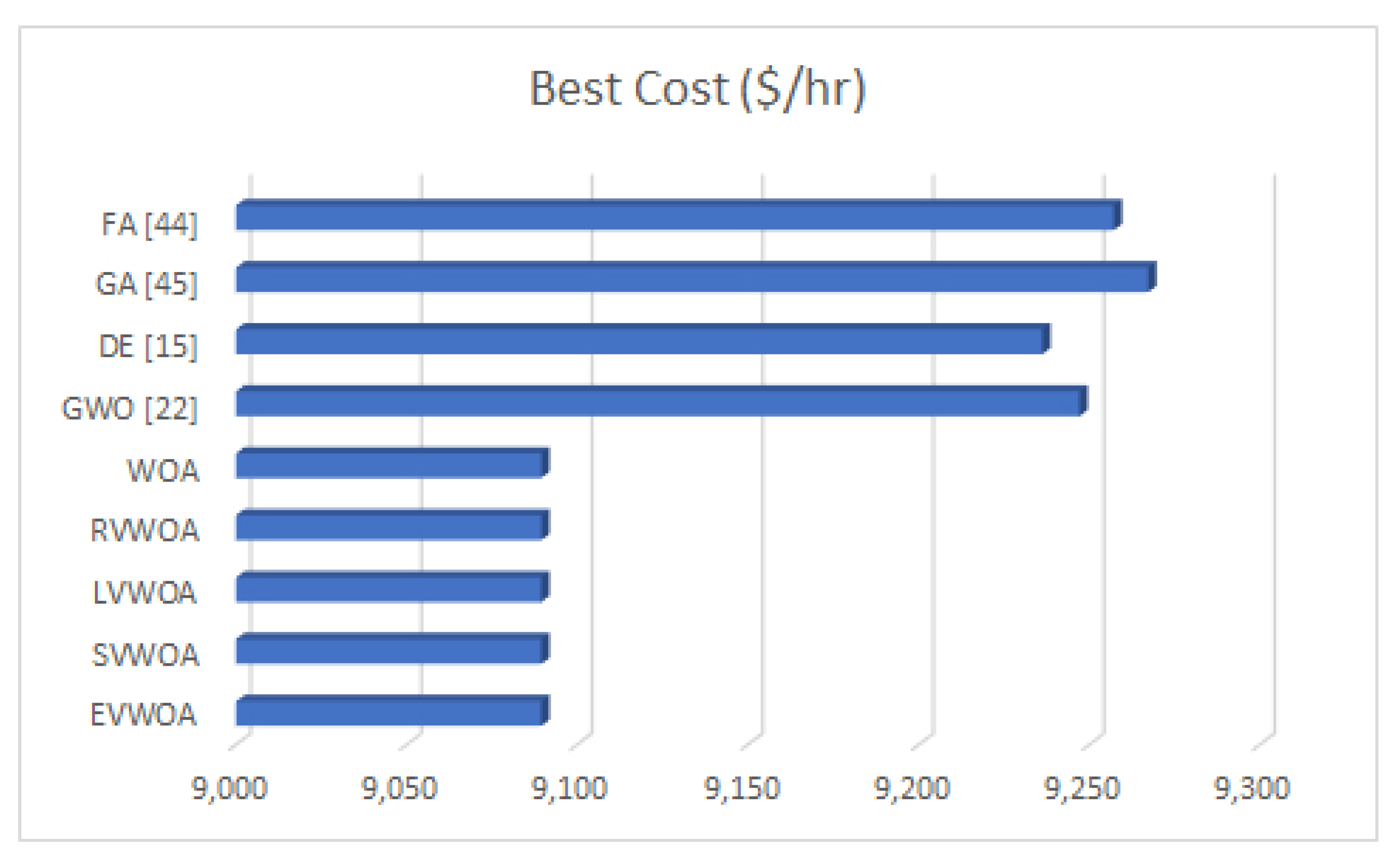
| FA [43] | 9257.1 | - | - | - | - |
| GA [44] | 9267.2 | - | - | - | - |
| DE [15] | 9236.14 | - | - | - | 1.0674 |
| GWO [22] | 9257.07 | - | - | - | 1.33 |
| WOA | 9089.446 | 9108.160 | 9496.51 | 0.019422 | 0.23 |
| RVWOA | 9089.440 | 9089.489 | 9089.498 | 0.000001 | 0.27 |
| LVWOA | 9089.432 | 9089.488 | 9089.497 | 0.000001 | 0.24 |
| SVWOA | 9089.429 | 9089.486 | 9089.497 | 0.000002 | 0.22 |
| EVWOA | 9089.420 | 9089.441 | 9089.442 | 0.000001 | 0.26 |
| P1 | P2 | P3 | P4 | H2 | H3 | H4 | H5 |
|---|---|---|---|---|---|---|---|
| 135 | 40.77 | 19.23 | 105 | 73.64 | 36.73 | 0 | 39.63 |
| Technique | Best ($/h) | Mean ($/h) | Worst ($/h) | STD | Time(s) |
|---|---|---|---|---|---|
| Cost | Cost | Cost | |||
| FA [43] | 13,683.22 | - | - | - | - |
| HS [45] | 13,723.2 | - | - | - | - |
| IWO [20] | 13,683.65 | - | - | - | 1.0674 |
| COA [46] | 13,672.83 | - | - | - | 1.33 |
| EMA [21] | 13,672.84 | - | - | - | 1.33 |
| WOA | 13,672.8211 | 13,686.0696 | 13,738.7084 | 0.001269 | 0.179 |
| RVWOA | 13,672.7970 | 13,673.5999 | 13,715.5134 | 0.000403 | 0.178 |
| LVWOA | 13,672.7964 | 13,673.4296 | 13,694.7275 | 0.000311 | 0.161 |
| SVWOA | 13,672.7961 | 13,673.1225 | 13,681.8538 | 0.000073 | 0.162 |
| EVWOA | 13,672.7889 | 13,672.7911 | 13,672.8052 | 0.000000 | 0.229 |
| P1 | P2 | P3 | P4 | P5 | P6 | H5 | H6 | H7 |
|---|---|---|---|---|---|---|---|---|
| 58.81 | 98.54 | 112.67 | 209.82 | 81 | 40 | 0 | 95.18 | 54.82 |
| Technique | Best ($/h) | Mean ($/h) | Worst ($/h) | STD | Time(s) |
|---|---|---|---|---|---|
| Cost | Cost | Cost | |||
| TLBO [13] | 10,094.84 | - | - | - | 2.86 |
| GSA [7] | 9912.69 | - | - | - | 2.578 |
| DE [48] | 10,317 | - | - | - | 5.26 |
| WOA | 9798.9957 | 10,025.0678 | 10,445.6392 | 0.015587 | 0.84 |
| RVWOA | 9745.6136 | 9820.6379 | 10,052.4499 | 0.005443 | 0.764 |
| LVWOA | 9742.9177 | 9819.7254 | 10,048.6937 | 0.005436 | 0.637 |
| SVWOA | 9741.0869 | 9818.4077 | 10,030.7712 | 0.004869 | 0.643 |
| EVWOA | 9739.5049 | 9810.4882 | 10,003.2598 | 0.004716 | 0.767 |
| P1 | 628.32 | P7 | 159.73 | P13 | 55 | P19 | 35 | H19 | 45 |
| P2 | 298.65 | P8 | 60 | P14 | 81 | H14 | 180 | H20 | 158.79 |
| P3 | 286.85 | P9 | 60 | P15 | 40 | H15 | 135.6 | H21 | 60 |
| P4 | 109.86 | P10 | 40 | P16 | 81 | H16 | 180 | H22 | 60 |
| P5 | 109.86 | P11 | 40 | P17 | 40 | H17 | 135.6 | H23 | 120 |
| P6 | 159.73 | P12 | 55 | P18 | 10 | H18 | 55 | H24 | 120 |
| Technique | Best ($/h) | Mean ($/h) | Worst ($/h) | STD | Time(s) |
|---|---|---|---|---|---|
| Cost | Cost | Cost | |||
| OTLBO [13] | 57,856.27 | 57,883.22 | 57,913.77 | - | - |
| EMA [21] | 57,825.48 | 57,832.74 | 57,841.15 | - | - |
| IGSO [49] | 58,049.02 | 58,156.52 | 58,219.14 | - | - |
| CSO [21] | 57,907.12 | 57,908.31 | 579,11.95 | - | - |
| WOA | 53413.4800 | 53,985.95 | 55,991.7200 | 0.011879 | 0.513 |
| RVWOA | 53,370.3314 | 53,766.9799 | 55,314.1664 | 0.005630 | 0.560 |
| LVWOA | 53,288.2511 | 53,737.1996 | 55,253.9625 | 0.005256 | 0.564 |
| SVWOA | 53,275.6137 | 53,730.6929 | 54,805.6054 | 0.004046 | 0.564 |
| EVWOA | 53,167.3683 | 53,373.1923 | 53,813.7479 | 0.002577 | 0.587 |
| P1 | 616.01 | P16 | 360 | 31 | 10 | H34 | 135.6 |
| P2 | 0 | P17 | 179.99 | P32 | 35 | H35 | 180 |
| P3 | 0 | P18 | 179.99 | P33 | 81 | H36 | 135.6 |
| P4 | 60 | P19 | 179.99 | P34 | 40 | H37 | 55 |
| P5 | 60 | P20 | 179.99 | P35 | 81 | H38 | 45 |
| P6 | 60 | P21 | 179.99 | P36 | 40 | H39 | 176.41 |
| P7 | 60 | P22 | 179.99 | P37 | 10 | H40 | 60 |
| P8 | 60 | P23 | 119.99 | P38 | 35 | H41 | 60 |
| P9 | 60 | P24 | 119.99 | H27 | 179.98 | H42 | 120 |
| P10 | 40 | P25 | 119.99 | H28 | 135.6 | H43 | 120 |
| P11 | 40 | P26 | 120 | H29 | 144.74 | H44 | 176.46 |
| P12 | 55 | P27 | 81 | H30 | 135.6 | H45 | 60 |
| P13 | 55 | P28 | 40 | H31 | 55 | H46 | 60 |
| P14 | 679.99 | P29 | 81 | H32 | 45 | H47 | 120 |
| P15 | 359.99 | P30 | 40 | H33 | 180 | H48 | 120 |
| Technique | Best ($/h) | Mean ($/h) | Worst ($/h) | STD | Time(s) |
|---|---|---|---|---|---|
| Cost | Cost | Cost | |||
| COA [46] | 116,789.92 | 116,835.55 | 117,068.27 | - | - |
| CSO [50] | 115,967.72 | 115,995.88 | 116,047.22 | - | - |
| MPSO [51] | 116,465.54 | 116,471.36 | 116,482.44 | - | - |
| GSO [52] | 116,457.96 | 116,463.65 | 116,473.22 | - | - |
| WOA | 99,136.8303 | 107,026.2565 | 116,304.7858 | 0.033216 | 0.471 |
| RVWOA | 99,136.8303 | 107,026.2565 | 116,304.7858 | 0.033216 | 0.471 |
| LVWOA | 97,958.8952 | 104,552.0051 | 111,761.6686 | 0.026202 | 0.559 |
| SVWOA | 97,774.6398 | 104,342.2406 | 111,088.5884 | 0.023165 | 0.540 |
| EVWOA | 92,887.876940 | 96,657.722614 | 105,615.720811 | 0.021991 | 0.617 |
| P 1 | 630.39 | P 21 | 109.69 | P 41 | 294.73 | P 61 | 81 | H 57 | 0.014 | H 77 | 0.014 |
| P 2 | 294.73 | P 22 | 109.91 | P 42 | 294.73 | P 62 | 40 | H 58 | 0.014 | H 78 | 0.014 |
| P 3 | 294.73 | P 23 | 40 | P 43 | 109.91 | P 63 | 10 | H 59 | 0.014 | H 79 | 0.014 |
| P 4 | 109.91 | P 24 | 40 | P 44 | 109.91 | P 64 | 35 | H 60 | 0.014 | H 80 | 0.014 |
| P 5 | 109.91 | P 25 | 55 | P 45 | 109.91 | P 65 | 81 | H 61 | 0.014 | H 81 | 0.014 |
| P 6 | 109.91 | P 26 | 55 | P 46 | 108.22 | P 66 | 40 | H 62 | 0.014 | H 82 | 2499.70 |
| P 7 | 109.91 | P 27 | 630.39 | P 47 | 109.69 | P 67 | 81 | H 63 | 0.014 | H 83 | 0.014 |
| P 8 | 109.91 | P 28 | 294.73 | P 48 | 86.79 | P 68 | 40 | H 64 | 0.014 | H 84 | 0.014 |
| P 9 | 109.91 | P 29 | 294.73 | P 49 | 40 | P 69 | 10 | H 65 | 0.014 | H 85 | 0.014 |
| P 10 | 40 | P 30 | 109.91 | P 50 | 40 | P 70 | 35 | H 66 | 0.014 | H 86 | 0.014 |
| P 11 | 40 | P 31 | 109.91 | P 51 | 55 | P 71 | 81 | H 67 | 0.014 | H 87 | 2499.70 |
| P 12 | 55 | P 32 | 109.91 | P 52 | 55 | P 72 | 40 | H 68 | 0.014 | H 88 | 0.014 |
| P 13 | 55 | P 33 | 109.91 | P 53 | 81 | P 73 | 81 | H 69 | 0.014 | H 89 | 0.014 |
| P 14 | 630.39 | P 34 | 109.91 | P 54 | 40 | P 74 | 40 | H 70 | 0.014 | H 90 | 0.014 |
| P 15 | 294.73 | P 35 | 109.91 | P 55 | 81 | P 75 | 10 | H 71 | 0.014 | H 91 | 0.014 |
| P 16 | 294.73 | P 36 | 40 | P 56 | 40 | P 76 | 35 | H 72 | 0.014 | H 92 | 0.014 |
| P 17 | 109.91 | P 37 | 40 | P 57 | 10 | H 53 | 0.014 | H 73 | 0.014 | H 93 | 0.014 |
| P 18 | 109.91 | P 38 | 55 | P 58 | 35 | H 54 | 0.014 | H 74 | 0.014 | H 94 | 0.014 |
| P 19 | 109.91 | P 39 | 55 | P 59 | 81 | H 55 | 0.014 | H 75 | 0.014 | H 95 | 0.014 |
| P 20 | 109.91 | P 40 | 630.39 | P 60 | 40 | H 56 | 0.014 | H 76 | 0.014 | H 96 | 0.014 |
| Technique | Best ($/h) | Mean ($/h) | Worst ($/h) | STD | Time(s) |
|---|---|---|---|---|---|
| Cost | Cost | Cost | |||
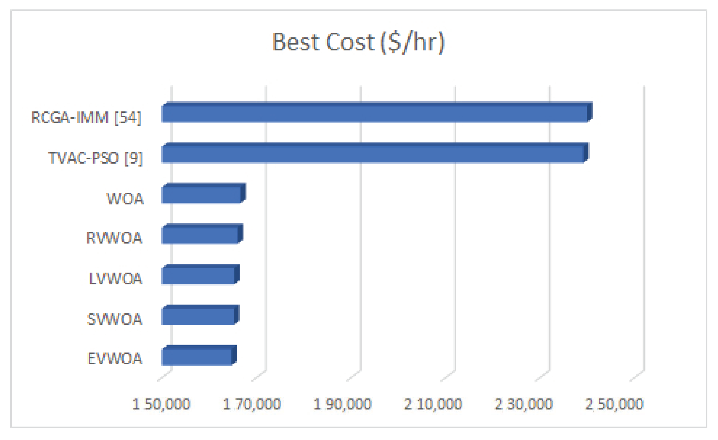
| RCGA-IMM [53] | 239,896.4082 | - | - | - | 280.47 |
| TVAC-PSO [9] | 239,139.5018 | - | - | - | 198.25 |
| WOA | 166,598.2166 | 172,476.1561 | 190,501.0311 | 0.019690 | 2.555 |
| RVWOA | 166,017.3783 | 170,507.9580 | 182,953.4631 | 0.018518 | 1.922 |
| LVWOA | 165,290.1180 | 170,003.9993 | 176,234.0878 | 0.014683 | 1.749 |
| SVWOA | 165,224.8771 | 168,008.8607 | 173,527.3772 | 0.010526 | 1.922 |
| EVWOA | 164,691.7101 | 167,690.1798 | 171,696.4346 | 0.008756 | 2.600 |
Publisher’s Note: MDPI stays neutral with regard to jurisdictional claims in published maps and institutional affiliations. |
© 2021 by the authors. Licensee MDPI, Basel, Switzerland. This article is an open access article distributed under the terms and conditions of the Creative Commons Attribution (CC BY) license (http://creativecommons.org/licenses/by/4.0/).
Share and Cite
Jadoun, V.K.; Prashanth, G.R.; Joshi, S.S.; Agarwal, A.; Malik, H.; Alotaibi, M.A.; Almutairi, A. Optimal Scheduling of Non-Convex Cogeneration Units Using Exponentially Varying Whale Optimization Algorithm. Energies 2021, 14, 1008. https://doi.org/10.3390/en14041008
Jadoun VK, Prashanth GR, Joshi SS, Agarwal A, Malik H, Alotaibi MA, Almutairi A. Optimal Scheduling of Non-Convex Cogeneration Units Using Exponentially Varying Whale Optimization Algorithm. Energies. 2021; 14(4):1008. https://doi.org/10.3390/en14041008
Chicago/Turabian StyleJadoun, Vinay Kumar, G. Rahul Prashanth, Siddharth Suhas Joshi, Anshul Agarwal, Hasmat Malik, Majed A. Alotaibi, and Abdulaziz Almutairi. 2021. "Optimal Scheduling of Non-Convex Cogeneration Units Using Exponentially Varying Whale Optimization Algorithm" Energies 14, no. 4: 1008. https://doi.org/10.3390/en14041008
APA StyleJadoun, V. K., Prashanth, G. R., Joshi, S. S., Agarwal, A., Malik, H., Alotaibi, M. A., & Almutairi, A. (2021). Optimal Scheduling of Non-Convex Cogeneration Units Using Exponentially Varying Whale Optimization Algorithm. Energies, 14(4), 1008. https://doi.org/10.3390/en14041008