1. Introduction
Over the past years, wind turbines have increased significantly in size in an effort to reduce the cost of wind energy and make it a competitive source of energy. So far, this has been a successful approach. An example of this success can be seen in the increased installation numbers of new wind turbines in Germany [
1]. Yet increasing the turbine size also has its drawbacks. A larger rotor will be subjected to higher aerodynamic and gravitational loads. For example, the aerodynamic bending moments and the moments due to the self-weight of the blade scale as the third and fourth power of the rotor diameter respectively ([
2], (pp. 97–123)). As a consequence, the structure of the turbine components such as rotor blades has to be stiffer, which requires more or stronger material. This leads to an increase in the cost of energy. A way of counteracting the load increase seen in larger wind turbines is through the use of advanced wind turbine controllers. This allows for less material use in the design of the different components and hence results in a decrease of the cost of energy.
The most common actuator used for load alleviation is the blade pitch actuator. This comes from it being already used in the power regulation strategy of modern turbines. Many advanced load alleviation strategies using pitch actuators have been proposed. One of the best-known ones is the Individual Pitch Control (IPC) strategy [
3], which commonly relies on the out-of-plane Blade Root Bending Moments (BRBM) of the individual blades as input signals. It has been used in combination with different input sensors—such as inflow sensors [
4,
5]—and also in combination with different actuators—such as active trailing edge flaps [
6,
7,
8,
9]. Other studies have studied advanced model-based [
10] or adaptive [
11] controllers for load alleviation. A controller that uses neural networks as part of its architecture has also been recently proposed in [
12].
Oftentimes, the results of these studies are difficult to compare and reproduce. This is partly because many research groups use self-developed baseline controller strategies as a basis for load reduction comparative studies. The source code of these controllers is rarely available. Alternatively, studies that use the NREL 5 MW Reference Wind Turbine (RWT) [
13] also use the baseline controller available in the model definition. This is an older controller—based on [
14,
15]—that offers limited functionality and is inconvenient to use with other turbine models. This is because the controller parameters are hard-coded in the source file and the controller has to be recompiled every time the parameters change.
As part of the UpWind Project, a more advanced baseline controller was developed which allows for better power tracking and smoother transitions between the operating regions. These features lead to better energy capture and to reduced loading compared to the NREL 5 MW controller. Many of the aforementioned features are also implemented in the Basic DTU Wind Energy Controller [
16].
In recent years, the wind energy community has started to address the problem of reproducible controller results by introducing several modern, open-source reference wind turbine controllers. Mulders and van Wingerden publish the Delft Research Controller (DRC) [
17], which is expanded by Abbas et al. into NREL’s Reference Open-Source Controller (ROSCO) [
18]. Meng et al. also extend the Basic DTU Wind Controller to form the DTU Wind Energy Controller (DTUWEC), which includes advanced industrial features [
19].
All of the cited reference controllers use classical controller architectures such as PID controllers. As discussed in ([
20], (pp. 506–518)), there are several reasons for this choice. An important one is that with classical controller architectures, controller stability can be guaranteed. This is of utmost importance since modern large wind turbines are expected to operate reliably under all circumstances with minimum supervision. Another reason is that individual features can be added to the controller without the need to re-calibrate the whole controller. Also, the integration of a supervisory controller is much more straight-forward when classical controller architectures are used. Other control techniques such as neural networks are powerful techniques that could potentially be used to solve specific control objectives. They are therefore well suited to be part of advanced controller features. They are however less appropriate as candidates for reference baseline controllers. Because of their black-box model nature, it is difficult to guarantee their stability, add specific features or integrate them with supervisory controllers.
Having a reference controller is one aspect of accurate and comparable load reduction estimation. In order to have a complete picture of the design loads of different wind turbine components, we need to simulate the wind turbine in realistic aeroelastic scenarios that often include controller faults or other unforeseen events. Current industry standards prescribe a large number of aeroelastic simulations of the complete turbine [
21]. These are grouped together into Design Load Case (DLC) groups, each considering a particular scenario in the wind turbine’s design life. Most of the aforementioned studies only include a selection of DLC groups, such as the power production DLC group. While being a good approximation for certain component’s loads, using a selection of DLCs will not give a complete picture of the load reduction capabilities of the different turbine controllers. This is in part because many of the available wind turbine controllers do not feature a supervisory controller. The latter oversees the pitch and torque controller and reacts to unforeseen events, shutting down if threshold values of certain signals are passed in order to ensure the structural integrity of the turbine components. Only a full load calculation according to industry standards will give an accurate estimate of the load reduction capabilities of advanced controller strategies.
Another important aspect for accurate load estimation is the use of appropriate models in the aeroelastic simulations. Current aeroelastic codes mostly rely on the Blade Element Momentum (BEM) aerodynamic model to calculate aerodynamic loads ([
20], (pp. 57–66)). BEM models are attractive because they are computationally inexpensive. Yet in order to capture the more challenging unsteady aerodynamic phenomena present in DLCs, BEM models require a series of engineering corrections. These corrections have been developed and tested so that they work for a wide range of operating conditions. If the wind turbine operates in a condition outside this range, then the BEM corrections could introduce inaccuracies and overestimate the aerodynamic loading on the turbine. Examples of this include turbine operation in extreme yawed conditions or inflow conditions that are inhomogeneous across the rotor. This could arise if the turbine is operating in the partial wake of another turbine, in sheared and/or turbulent inflow due to the Earth’s boundary layer or if there is a large difference in the individual pitch angles of the blades (e.g., with pitch actuator faults) [
22,
23,
24,
25].
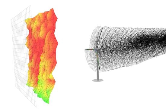
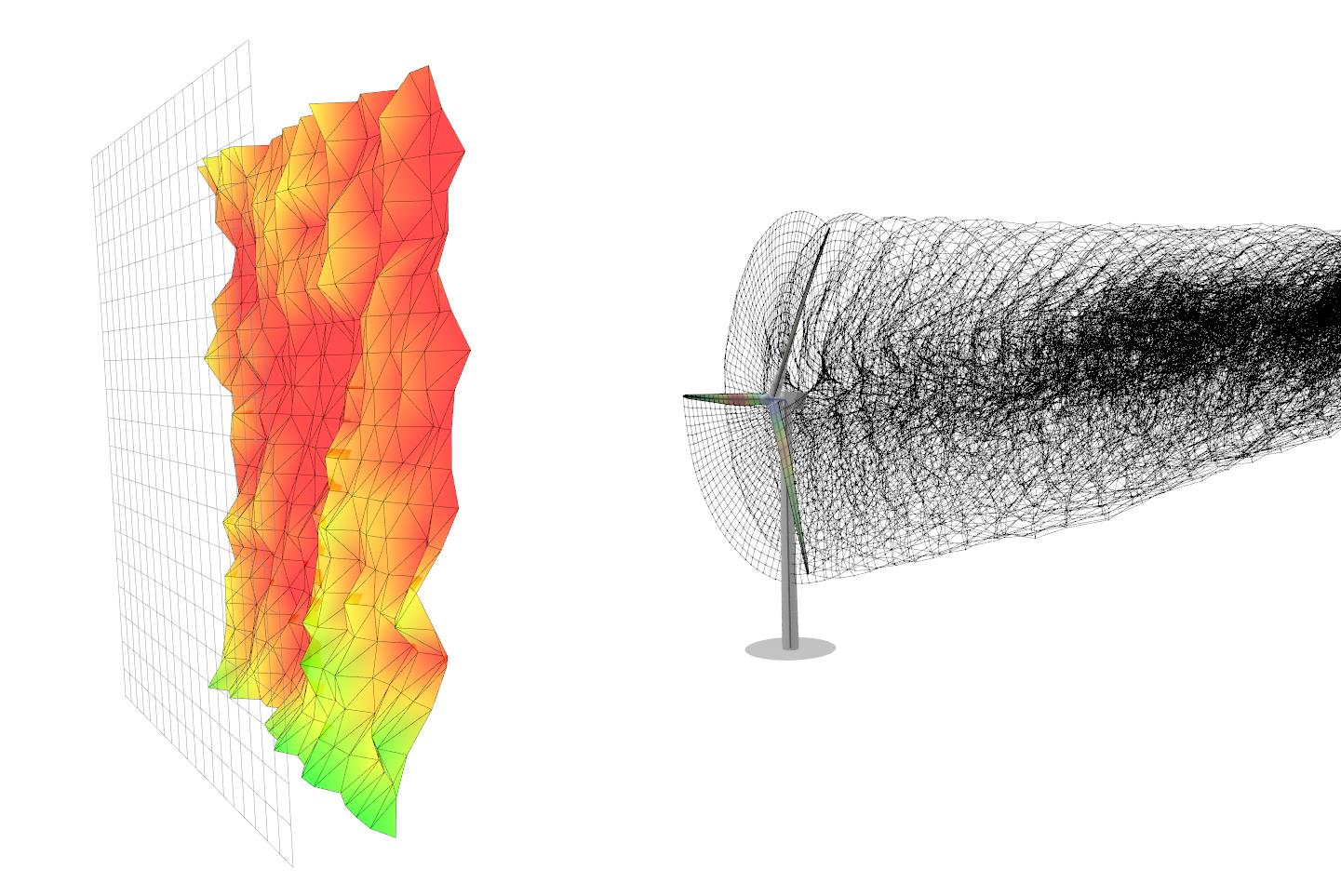
Vortex methods such as the Lifting Line Free Vortex Wake (LLFVW) aerodynamic model have a higher order representation of the unsteady aerodynamic phenomena and are capable of modeling these with far fewer assumptions than BEM models [
26]. This is because in the LLFVW method the wake is explicitly modeled. In [
27] the authors show that there are significant differences in fatigue and extreme loading if the aeroelastic simulations are performed with a BEM aerodynamic model compared to a LLFVW model, with the BEM model predicting increased fatigue loads. If we wish to accurately asses the load reduction potential of advanced control strategies based on individual pitch action, we require an accurate representation of the local aerodynamic effects that occur on each blade. Since the advanced controller action will be individual on each blade, the resulting induction field will be non-homogeneous. This in turn requires a higher-order aerodynamic model such as the LLFVW model to accurately estimate the effect of the resulting aerodynamic loads.
In this study, we address the aforementioned issues by introducing the TUB Controller (TUBCon). It is an open-source reference wind turbine controller with advanced load reduction strategies that features a complete supervisory controller. It can therefore be used to perform a full load calculation so that an accurate load picture of the turbine loads is obtained. Furthermore, this controller is fully compatible with the aeroelastic software QBlade [
28]—which features the LLFVW aerodynamic model. In combination, QBlade and TUBCon can be used to accurately calculate wind turbine loads and also evaluate the performance of advanced load reduction strategies. We give an example of this by analyzing the load reduction capabilities of the well-known IPC strategy in power production with turbulent wind conditions. This paper is structured as follows: In
Section 3 we present and fully describe TUBCon, including its advanced load reduction strategy and supervisory controller. In
Section 4, we validate TUBCon in steady and turbulent wind conditions by comparing its performance to an established wind turbine controller from the literature. In
Section 5 we analyze TUBCon’s advanced load reduction capabilities in turbulent wind conditions by simulating a reference wind turbine using the baseline and IPC variants of TUBCon. Conclusions are drawn in
Section 6.
3. Description of the TUB Controller
This section describes the TUB Controller (TUBCon). A graphical representation of the controller architecture is shown in
Figure 1.
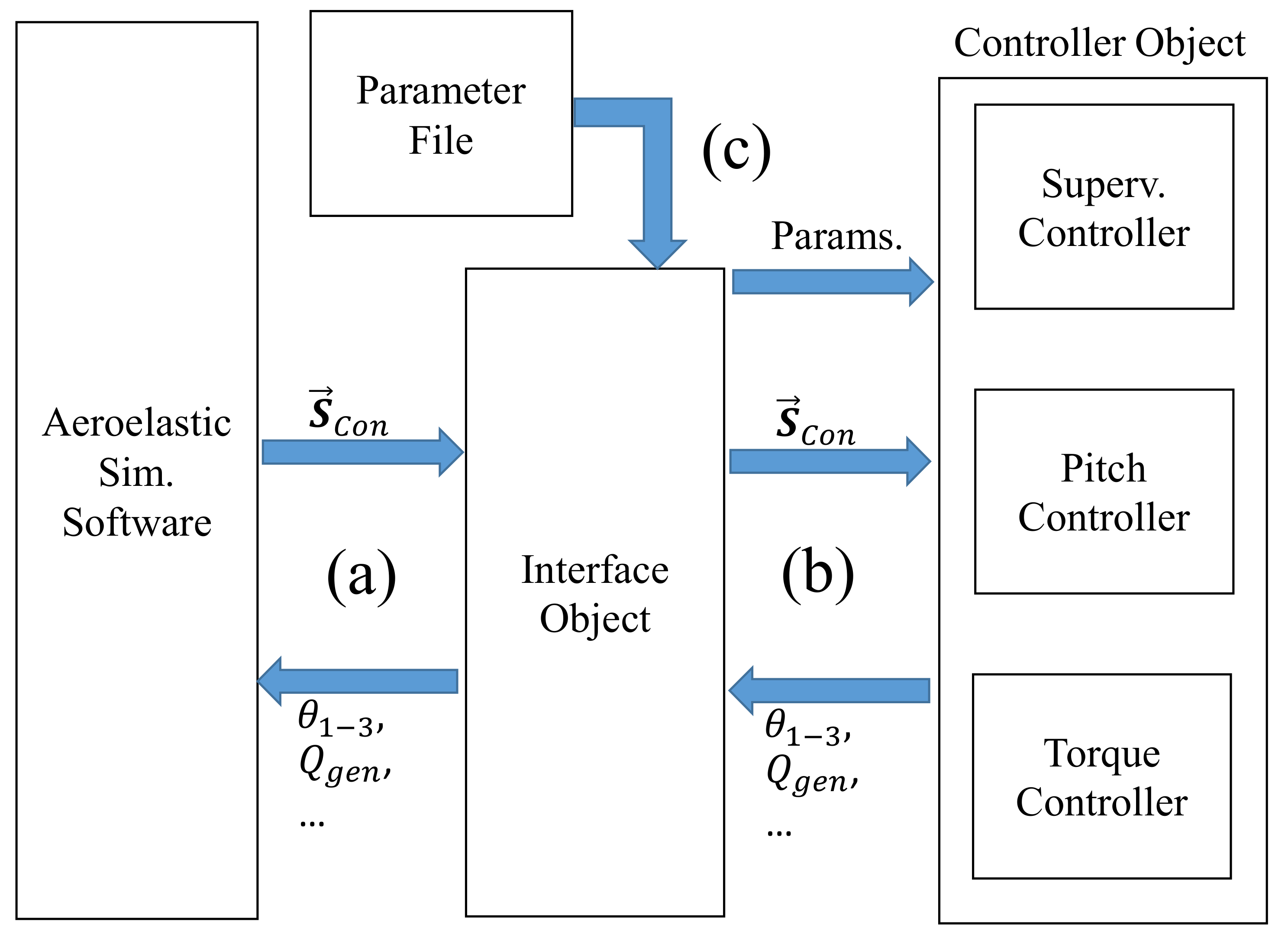
The controller code is written in C++ in an object-oriented manner. It features a two-stage interaction with the aeroelastic simulation software. The first stage is an interface object that handles the data exchange with the aeroelastic code (
Figure 1(a)). The current supported interfaces are the conventional Bladed-Style communication via a swap-array and a modified swap-array communication specially designed for interacting with QBlade. This makes TUBCon compatible with common aeroelastic simulation codes including OpenFAST, Bladed and QBlade. The modular nature of the interface object makes it easy to extend the compatibility of TUBCon with other aeroelastic codes.
The interface object then communicates with the turbine controller in a second stage
Figure 1(b). The individual controller components are designed in Simulink and compiled to a C++ object using the Simulink Coder package. The resulting object has an initialization function, a step function and a termination function. These are called by the main routine at the appropriate simulation times. Such an architecture allows us to rapidly develop and test new controller features that can be incorporated to the compiled controller library. The controller is parameterized externally using an appropriate parameter file (
Figure 1(c)). This XML file is read and the controller parameters set as part of the initialization routine.
The controller object is adapted from the Basic DTU Wind Energy Controller [
16] and shares many of its capabilities. It features a state-of-the-art pitch and torque controller that enable the turbine to operate reliably under unsteady turbulent wind conditions. Although the description of the torque and collective pitch controller is given in [
16], it is also included here for the sake of completeness.
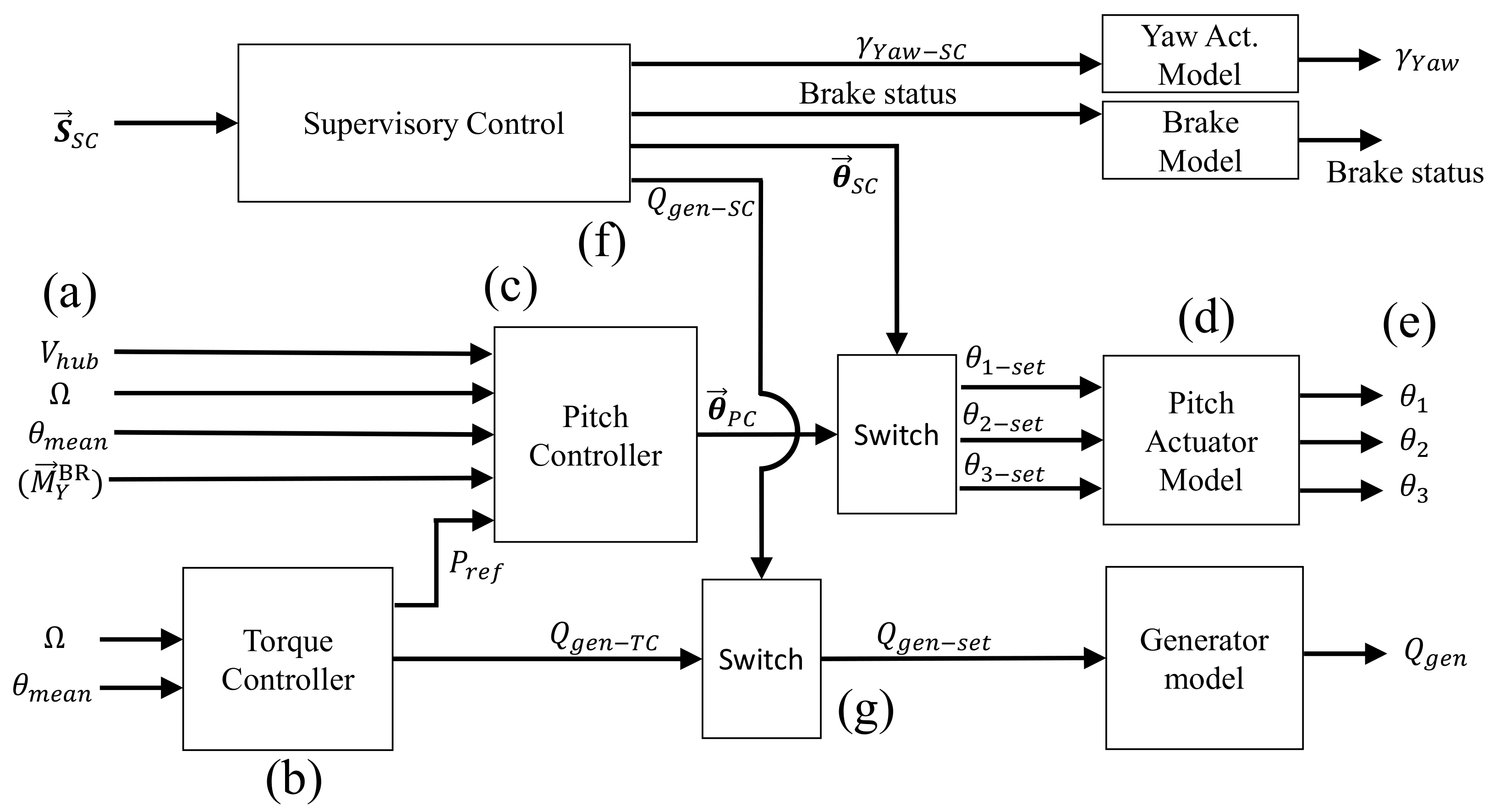
Figure 2 shows a schematic overview of the controller.
Both the pitch and torque controllers share the rotor speed
and the mean pitch angle
as input sensors (
Figure 2(a)). The output of the torque controller is the generator set-point torque
and the reference power
. The pitch controller uses the aforementioned
and
as well as
and the measured wind speed at hub height
to determine the set-point angles of all three blades (
and
) (
Figure 2(c)). If the IPC strategy is enabled, then the pitch controller also needs the out-of-plane BRBM of all blades (
). The controller includes actuator models for the pitch and yaw actuators as well as the brakes and generator to model the dynamics of the different actuators (
Figure 2(d)). The set-point signal of each controller is passed to the respective actuator model to calculate the actual signals passed back to the aeroelastic code (
Figure 2(e)). In the following sections, the individual parts of the controller will be further explained.
Figure 2 also shows the supervisory control. It is included to allow the controller to perform full load calculations. It will be explained in
Section 3.3 and is included in
Figure 2(f),(g) to show the location where the supervisory control overrides the signals of the individual controllers.
The pitch and torque controllers explained in the following sections operate using the low speed shaft side of the drive train. That is, they assume that the generator speed and torque are identical to the low speed shaft speed and torque. For geared turbines, the gear box ratio G is applied to convert the high speed shaft quantities into low speed shaft quantities and back.
3.1. Torque Controller
The torque controller is divided into two main parts: the partial and the full load regimes. There is also the switching logic to change between both regimes. The input for the controller is the rotor speed and the mean pitch angle . The latter is used for the switching logic between the two load regimes. The output of the controller is the generator torque and the reference power for the pitch controller. The reference power is simply the product of the instantaneous generator torque and the rotor speed: .
The variable speed controller is a PID controller with two different rotor speed set-points. The controller is saturated with a maximum and a minimum limit so that is adjusted to follow an optimum tip speed ratio in the partial load regime.
As a first step, the rotor speed
is low-pass filtered with a second order low-pass filter to exclude unwanted high frequency dynamics. The function of the low-pass filter is given by
Appendix A Equation (
A2). The speed error
is calculated using the difference of the low-passed rotor speed
and the current speed set-point
:
. The speed set-point is defined as
where
and
represent the rated and minimum rotor speed. The generator torque is computed using the equation
Here,
,
and
represent the proportional, the integral and the differential gain of the PID controller. Because the values of the generator torque are saturated, each time step, the integral term of
is recalculated as
This helps to avoid windup of and enables the controller to react quickly if the required torque signal changes from a previously saturated value.
3.1.1. Partial Load Regime
In order for the torque controller to enforce an optimum tip speed ratio in the partial load regime, the generator torque is saturated with upper and lower limits:
and
. Between
and
, the limits are identical and follow the optimal torque speed curve of the turbine:
In the last equation, represents the air density, R the rotor radius and the power coefficient at optimum tip speed ratio .
At two given rotor speed ranges,
and
, the torque limits open up to allow the PID controller to keep the rotor speed at the required set-point. The switching logic for
is given by:
In the above equation,
represents the generator torque in full load regime and
represents a smooth switching function between the two limits
and
. The switch function is given by Equations (
A5) and (
A6). Complementary to Equation (
6),
follows the switching logic:
The above equation uses the symbol to denote the switch function .
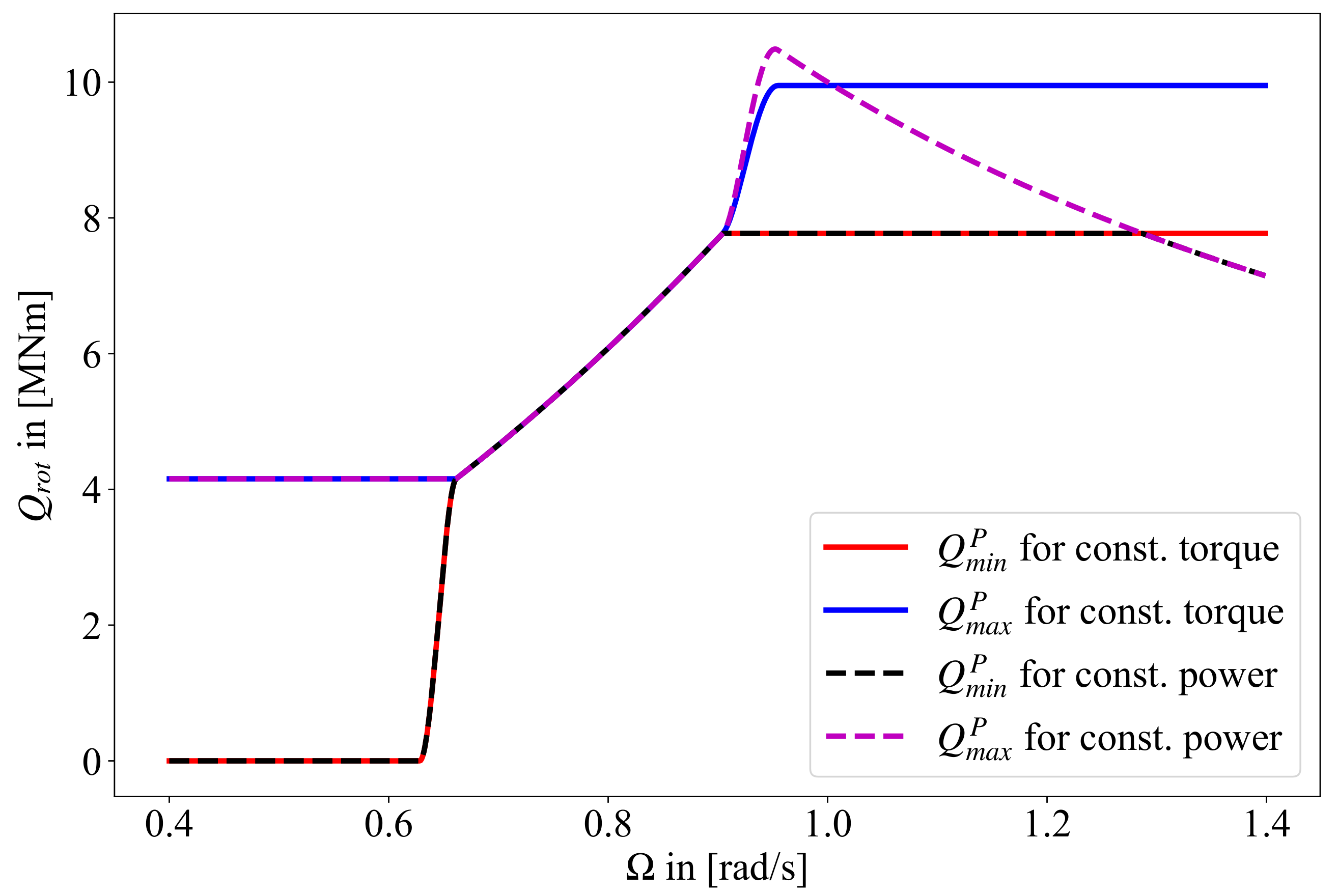
Figure 3 shows the torque limits as a function of
.
Below the minimum rotor speed,
is kept at 0 kNm to allow the rotor to gain enough rotational speed at low wind speeds. Once the rotor speed reaches
(95% of
in the figure),
is increased and equaled to
. This enforces the optimal torque-speed curve of the wind turbine below the rated speed. Once
gets close to
(95% of
),
opens up to allow the PID controller to regulate the rotor speed. The parameters
and
are externally defined by the user.
Figure 3 includes the behavior of the torque limits for the two torque control strategies in the full load regime: constant power and constant torque. These are explained in the next section.
3.1.2. Full Load Regime
The full load regime of the controller uses the same PID controller for the controller torque, but now the torque limits
and
take the same value
. The control strategy of the torque controller in the full load regime can be either constant power or constant torque.
takes different values depending on the strategy. These are:
While
is constant for the constant torque strategy, it is inversely proportional to the (unfiltered) rotor speed signal for the constant power strategy. This explains the
behavior of
and
for the constant power strategy in
Figure 3.
3.1.3. Switching between Regimes
The controller switches between partial and full load regimes depending on the first order low-pass filtered switch variable
.
is defined using Equation (
A5) as
. The limits
and
are user-defined parameters. For this study, the limits were defined as
. In this configuration, the switching function
behaves like a step function. The variable
is the minimum pitch angle of the pitch controller, defined in
Section 3.2. The equation of the first order low-passed filter is given by (
A1).
Including the switching between regimes and the torque strategy in the above rated regime, the full torque limits take the form
3.1.4. Drivetrain Damper
The torque controller also includes a drivetrain damper to damp unwanted oscillation of the turbine shaft due to e.g., excitation of its torsional eigenfrequency. The drivetrain damper is implemented as a proportional term
to the band-passed rotor speed signal
:
The equation of the band-pass filter is given in Equation (
A3).
is added to
to obtain the total output torque of the controller:
3.1.5. Disable for Low Rotor Speeds
An additional feature of the controller is a switch-off mechanism for low rotor speeds. The rotor speed signal
is filtered using a low pass filter (see Equation (
A2)) and compared to a fraction of the minimum rotor speed:
. If the filtered rotor speed signal is below this value, then the torque controller shuts down by setting
Nm. Note that if the turbine rotor speeds up again and the (filtered) rotor signal exceeds the aforementioned limit, then the torque controller is activated again and functions as described above.
3.2. Pitch Controller
The pitch controller in TUBCon features two strategies. The first is the Collective Pitch Control (CPC) strategy for power regulation. The second is the advanced Individual Pitch Control (IPC) strategy for additional load reduction. The CPC strategy is always active while the IPC strategy can be enabled by the user through the external parameter file.
3.2.1. Collective Pitch Control
The CPC controller combines two PID controllers that react to the rotor speed error and the power error. The inputs for the pitch controller are the rotor speed
, the mean pitch angle
, the reference power from the torque controller
and the measured wind speed at hub height
(see
Figure 2(a)).
The rotor speed signal is filtered using a second order low-pass filter as described by Equation (
A2). Both the pitch and the torque controller share the same filter frequency and damping ratio to calculate
. The speed error
is calculated as the difference between the low pass filtered rotor speed
and the rated rotor speed
. The error
is then passed through a notch filter to filter out the drivetrain eigenfrequency. The equation of a notch filter is given in Equation (
A4).
In parallel, the power error
is calculated as the difference between
and
and passed through a notch filter (Equation (
A4)) to obtain
. The proportional, integral and differential terms of the pitch controller are calculated as follows:
Here, and are the proportional, integral and derivative constants of each PID controller. The subscript denotes that the PID constants are applied to . Likewise, the subscript P denotes the affiliation of the constants to . Note that is always set to zero.
Additionally, the pitch signal is gain-scheduled with two factors. The first one accounts for the non-linear effect that larger blade pitch angles have on the aerodynamic torque. The second factor increases sensitivity of the pitch controller to large speed excursions in order to limit them. The total gain schedule is calculated via
In this equation,
is the low-pass filtered mean pitch signal
.
and
are parameters given by the user. To calculate
, a first order filter as described in Equation (
A1) is used.
The pitch angle signal is limited by the parameters
and
. In addition,
can be modified by
using a look-up table given by the user. In this case, the measured wind speed at hub height is also low-passed using a first order low pass filter (Equation (
A1)).
In order for the pitch controller to react quickly if the required pitch signal changes suddenly from a saturated value, an anti-windup scheme like the one described in Equation (
3) is used for
.
The total collective pitch angle signal of the pitch controller is therefore given by
Additionally, the pitch rate is also limited by two user defined parameters: and .
The power dependency of
will make the pitch controller raise the pitch angle set point when
from the torque controller is close to
. This in turn helps trigger the switching procedure from partial to full load regime of the torque controller as explained in
Section 3.1.3.
3.2.2. Individual Pitch Control
One of the most common advanced pitch control strategies in wind energy research is the Individual Pitch Control (IPC) strategy [
3,
33]. Several studies have used this strategy as a comparison to other advanced pitch controller strategies [
4,
11,
34]. It has also been used as a comparison or a complementary strategy for trailing edge flap controllers [
7,
9,
10].
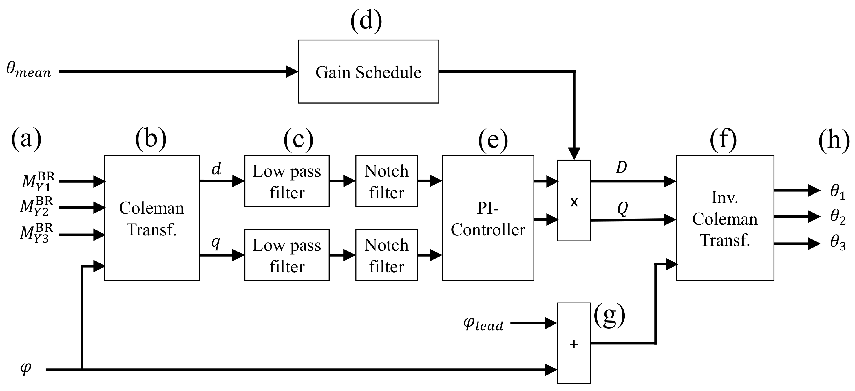
Figure 4 shows the graphical representation of the IPC strategy implemented in TUBCon.
The IPC uses as input signals the out-of-plane BRBM of the three blades (
) as well as the mean pitch angle
and the rotor azimuth angle
(
Figure 4(a)). The out-of-plane BRBMs are transformed to the direct and quadrature axes using the once-per-revolution or 1P-Coleman transformation (
Figure 4(b)). The 1P-Coleman transformation for a three bladed rotor takes the form
where
d and
q are the quantities expressed in the direct and quadrature axes respectively. The physical interpretation of these quantities is the rotor tilt and yaw moment in the non-rotating coordinate system.
These rotor moments are then passed through a second order low-pass filter (Equation (
A2)) and a notch filter (Equation (
A4))
Figure 4(c) to filter out unwanted high frequency content as well as the 1P component of the load signals in the non-rotating frame of reference. This step is needed as a 1P oscillation in the non-rotating frame of reference can lead to an increased 3P excitation of the turbine [
35]. Following a concept presented in [
9], a gain schedule is implemented using
to adapt the individual pitching action to the wind speed (
Figure 4(d)). The gain schedule has the same mathematical expression as
in Equation (
16) but uses different parameter values. A PI controller is implemented with a zero set-point to reduce the rotor tilt and yaw moments (
Figure 4(e)).
The control demand is transformed back to the demands of the individual pitch angles using the inverse 1P-Coleman transformation (
Figure 4(f)). The inverse transformation is given by
where the quantities
D and
Q represent the control signals in the non-rotating coordinate system and
,
and
the individual pitch angles for each blade (
Figure 4(h)). The inverse Coleman transformation uses a modified azimuth angle
.
Figure 4(g) shows that
, where
is the lead angle. This constant angle helps decoupling the rotor yaw and tilt moments in the non-rotating frame of reference so that they can be treated as independent systems. As explained in [
4], certain factors such as blade stiffness, collective pitch angle and pitch actuator response time introduce a dependency between the two rotor moments. Using the lead angle is a straightforward way to counter this problem.
It is possible to generalize this strategy to other frequencies by using
nP Coleman transformations. In this case the rotor angle
and the respective shift for each blade in Equations (
18) and (
19) are replaced by
n-times their value. Using for example an IPC-like strategy with a 2P Coleman transform helps to reduce the 3P asymmetrical loads in the yaw bearing of the turbine [
10].
The IPC pitch angles are limited to a maximum and minimum value (
and
) given by the user. Since the PI controller determines the quantities
D and
Q in the non-rotating coordinate system, the limits are transformed into this coordinate system:
As with the CPC strategy, an anti-windup procedure equivalent to Equation (
3) is used to limit the increase of the integral part of the controller.
The pitch angle signal of the IPC strategy is added to the collective pitch signal to obtain the final pitch angle signal. The use of this strategy increases the pitch activity significantly. In order to limit this increase in pitch activity, the control strategy is phased out in the partial load regime. Bergami and Gaunaa show in [
36] that the majority of fatigue loading that can be alleviated with this strategy occurs in the above-rated region. Phasing out the IPC strategy helps limit the pitch activity and optimizes energy capture by keeping the pitch angle constant in the below-rated region. The phasing out is done by multiplying the IPC PI-constants with a switch function (Equation (
A5)) based on
. The switch limits used in this study are
and
.
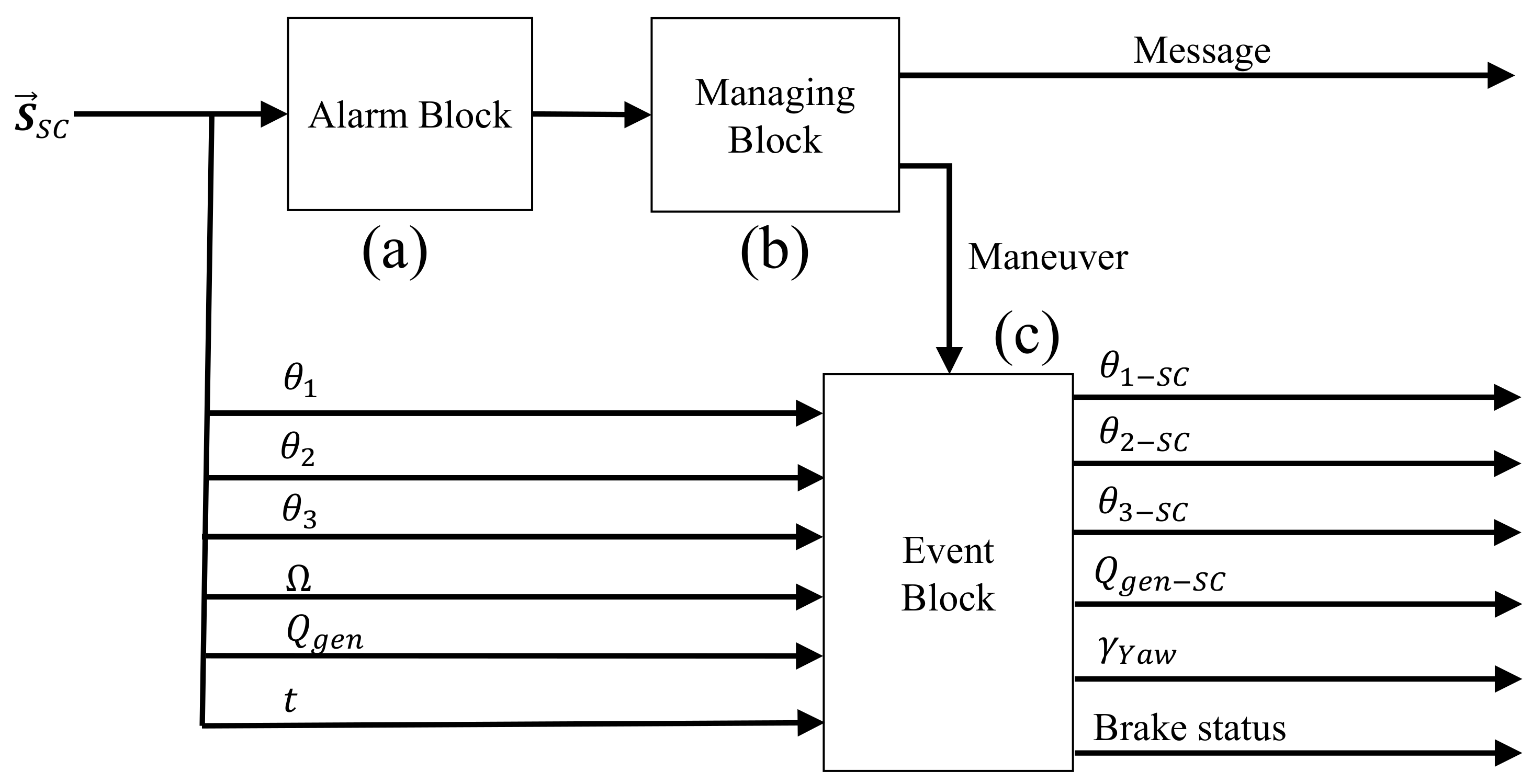
3.3. Supervisory Control
The supervisory control of TUBCon has two main functions. The first one is to detect whenever some security limit (e.g., generator over-speed) has been tripped and enforce an appropriate maneuver (e.g., normal stop). The second function is to trigger specific events. These can be controller fault events (as required by current industry standards) or stop maneuvers (if a specific alarm has been triggered).
The control signals from the supervisory control will always override the signals from the pitch and torque controllers. This is shown in
Figure 2 with the switch for each controller. In this figure,
represents the pitch signal from the supervisory control that overrides the signal from the pitch controller. In the same manner,
overrides the generator torque from the torque controller. In addition, the supervisory controller can activate the brake and the yaw actuator of the turbine.
The internal logic of the supervisory control is based on [
37] and shown here in
Figure 5. It features three control blocks. The first one checks if any turbine sensor is outside its allowable range and triggers an alarm should this happen (
Figure 5(a)). The turbine sensors are bundled into the vector
in
Figure 5 for the sake of clarity (see
Section 3.3.1 for a full description of the considered sensors). Depending on the situation, the alarm can have several levels. An example of this could be the tripping of the first over-speed limit and the tripping of the second over-speed limit, both alarms depending on the sensor
.
The second block manages the alarms that the first block triggered and sets an appropriate reaction maneuver (
Figure 5(b)). Keeping the example above, if the alarm block detected a first over-speed trigger, the managing block would request a normal stop of the turbine. If a second over-speed trigger is detected, then the manager block would request an emergency stop procedure. The latter clearly has a higher priority than the former. Both stop procedures have a higher priority than the normal control action of the controller.
The third block is the event generator block (
Figure 5(c)). This block creates the necessary controller signals to simulate any given event. These signals could be a controller fault required by a specific design load case or the normal stop maneuver requested from the manager block. The input signals for this block are the current pitch angle of each blade
, the rotor speed
and torque
and the current time
t. The last sensor is needed if an event is to occur at a specific simulation time. The output of the event block are the overridden controller signals. Note that depending on the specific event, not all control signals are necessarily overridden.
3.3.1. Considered Alarms and Reaction Maneuvers
Table 1 lists all the considered alarms of the supervisory control. The first column shows the measured sensor, the second column the limit and the third column the requested maneuver. In the third column, NS stands for normal stop and ES for emergency stop. These are the only two currently implemented maneuvers of the controller and are explained below.
The alarm block considers five sensors: rotor speed , electrical power P, yaw misalignment , pitch angles and grid status. Both and P have two limits (n4, p4 and nA, pA respectively) that, when surpassed, trigger instantly the appropriate stop maneuver. The same simple trip-logic is implemented for the grid status signal. At the instant that the grid status is measured as offline, a normal stop maneuver is triggered.
For the other sensors, the alarm is triggered if the sensor surpasses the limit for a given time period. The alarm block foresees two limits for
with two different duration times. The first limit
considers long-time yaw misalignments. The measured yaw misalignment
has to be larger than this limit for a time interval greater than
, which should be fairly large. In contrast,
considers short-term extreme yaw misalignments. The yaw misalignment signal used to trigger the alarms is filtered with a first order low pass filter (Equation (
A1)) to even out variations coming from inflow turbulence.
For the pitch angle group, there are two conditions that can trigger alarms. The first one is the difference between the individual pitch angles (
or
). This difference is calculated differently depending on the active pitch control strategy. For the CPC strategy (
Section 3.2.1), the alarm block checks the difference between all three angles. If the difference between any two pitch angles is greater than the fixed limit
for a given time
, then the alarm is triggered and a normal stop maneuver is requested. For the IPC strategy (
Section 3.2.2), the pitch angle differences are measured against the collective pitch angle signal. The limit
is not constant but varies depending on the short-term mean difference between the IPC angle and the collective pitch angle (plus a used-defined offset angle). The short-term mean difference of the individual pitch angles is obtained by applying a first-order low pass filter to the instantaneous mean difference. The time constant for this filter is a user-defined parameter. By using this triggering strategy, the supervisory control can detect pitch angle faults even when the difference between two pitch angles lies below the maximum allowed pitch difference for the IPC strategy.
The second condition included in the pitch angle alarm group is the difference between the measured and the demanded pitch angle for each blade . If the difference between the two signals in any blade is greater than for a given time , then the alarm is triggered and a stop maneuver is requested.
The two stop maneuvers used in this controller are defined by a sequence of actions that are taken (almost) independently of the controller signals. The only exception is the normal stop maneuver that additionally uses the pitch angle differences, as explained below. The parameters for both maneuvers are listed and explained in
Table 2. Note that there are two sets of parameters: one for the normal stop and one for the emergency stop procedure.
The implemented stop maneuvers foresee that the collective pitch angle will increase at a rate up to a maximum value . This pitching towards feather can be delayed for a given time using the parameter . Parallel to the pitch controller, the torque controller decreases linearly to at a rate given by the parameter . This procedure can also be delayed for a given time using the parameter . In case of a grid loss, a chopper can keep the generator torque constant for a given time in order to avoid very high rotor speeds. There is also the option to enable the turbine brake during the stop maneuvers. This is controlled with an enable flag and a minimum rotor speed () at which the brake is activated.
In addition to these fixed parameters, the normal stop procedure checks the pitch angle differences between all blades. If the absolute value of a given difference is above 0.5°, then the pitch rate is replaced by the minimum value between and . This is done for all blades except the one with the highest pitch angle. This way the pitch angle differences are minimized during the stop maneuver avoiding unnecessary oscillations due to aerodynamic imbalances of the rotor. The emergency stop does not have this feature as it is designed to be hard coded in the turbine’s safety mechanism.
3.3.2. Considered Events
The event block allows the controller to simulate the events required by the current industry standards for a full load calculation [
21].
Table 3 presents and explains all the events that the controller is able to perform. All of the listed events are controlled by a set of parameters passed to the controller.
Both the normal stop and the emergency stop events require two parameters: a flag to indicate if the event will be triggered and the time at which the maneuver is triggered.
The pitch runaway to feather/fine fault simulates an error in one or several pitch actuators. In this event, one or several blades suddenly pitch with a given pitch rate to the respective extreme value. The pitch rate is one of the parameters for this event. The sign of the pitch rate defines if the event is a pitch-to-feather (positive rate) or a pitch-to-fine (negative rate) fault event. There is one activation flag and one activation time parameter for each blade. This gives the flexibility to simulate the single pitch fault events and the collective pitch fault events with a limited set of parameters.
The pitch transducer fault simulates an error in the measurement of the generator speed. Instead of the actual speed, the transducer measures a constant value and passes it to the pitch and torque controller. The parameters for this event are a flag to enable the event, the time at which the event starts and the constant generator speed passed to the controller once the fault occurs.
The grid loss event simulates a sudden loss of the electrical grid. As a consequence, the generator cannot feed the generated power to the grid and the torque drops to 0 Nm. This event also raises the grid loss flag so that the alarm block recognizes the event and triggers the appropriate maneuver. The parameters that control this event are a flag that enables it and the time at which the grid loss event happens.
Finally, the yaw runaway event simulates a malfunction in the yaw system that causes the yaw motor to activate. The parameters for this event are an activation flag, a time to start yawing, a yaw rate and a time to stop yawing.
3.4. Actuator Models
Once the set-point values of the blade pitch angles and generator torque are calculated by the respective controllers, they are passed to the actuator models of the controller (see
Figure 2). The actuator models are used to model the additional inertial effects of the physical actuators. These models can be very accurate depending on the individual needs of the calculation.
For the TUB Controller, a simple second-order linear model was chosen to model both the pitch actuators and the generator model. The second-order model has the same mathematical description as a second-order low-pass filter, namely Equation (
A2). This model is also used for the yaw actuator in the yaw runaway event. The individual cut-off frequencies and damping ratios for the actuators and the generator model are supplied as parameters by the user. For the brake actuator, a simple first-order linear model as described by Equation (
A1) is used. The time constant is supplied by the user.
3.5. Supervisory Control Event Examples
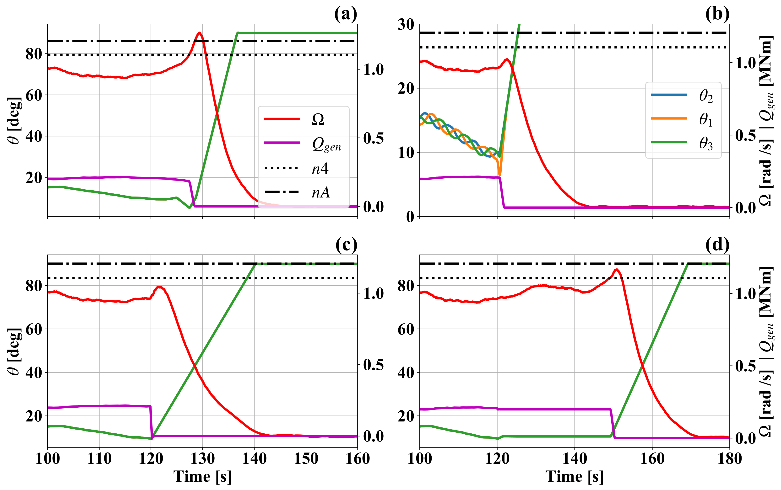
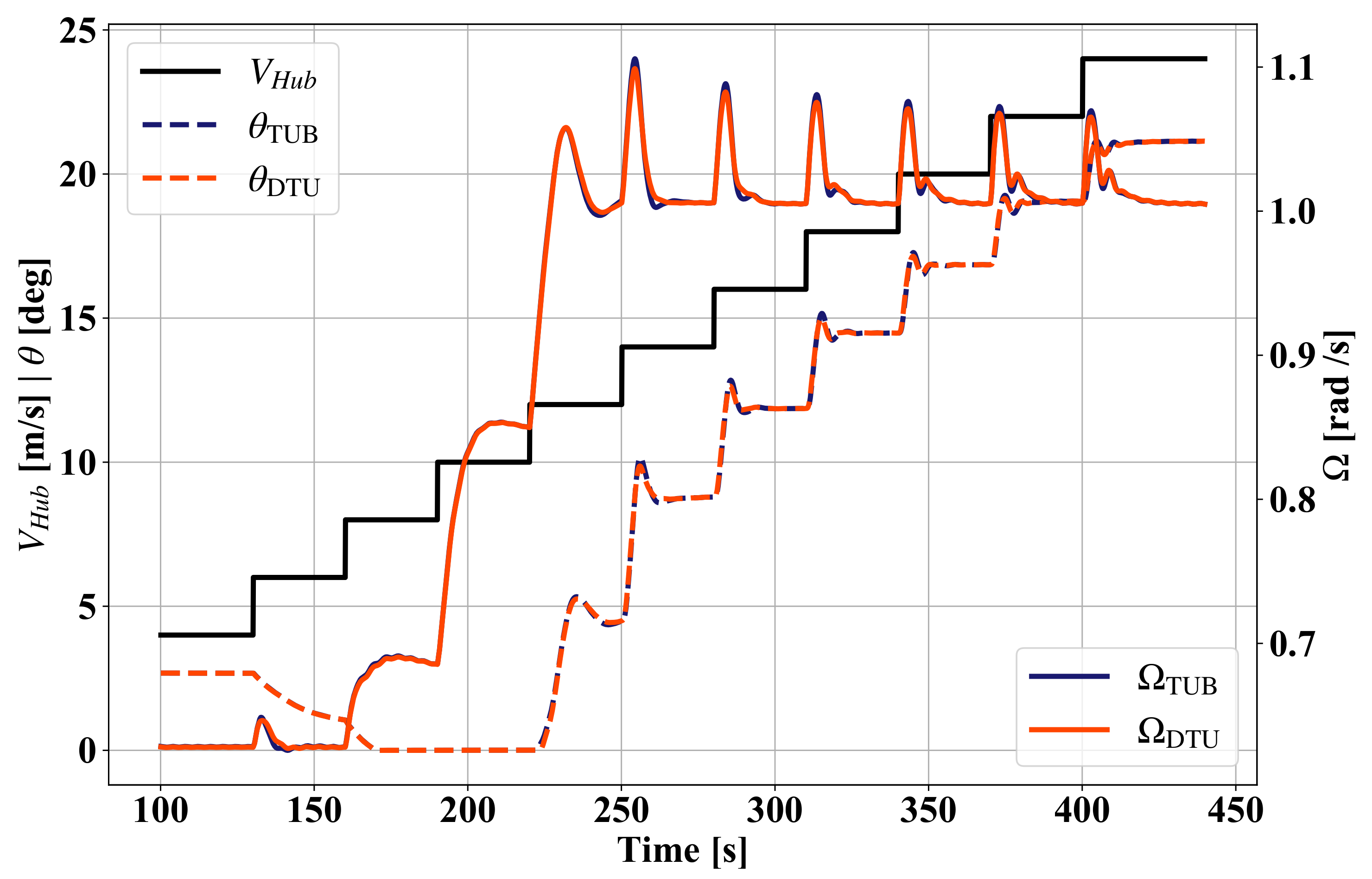
Figure 6 shows four examples of events and stop maneuvers using the DTU 10 MW RWT in turbulent wind simulations. In
Figure 6a, a collective pitch-to-fine fault at a simulation time of 125 s leads to the triggering of the first and second over-speed alarms. The resulting maneuvers (normal and emergency stop) can be distinguished by the different pitch rates.
Figure 6b shows a single pitch-to-fine event during power production using the IPC strategy. At 120 s of simulation time,
receives a faulty signal and starts pitching towards 0°. This is caught by the supervisory controller and the normal stop procedure is triggered. The normal stop feature that minimizes aerodynamic imbalances can be clearly seen in this figure, as the difference in individual pitch angles is reduced to 0° at 130 s of simulation time.
Figure 6c shows a grid loss scenario and the resulting stop maneuver. Finally,
Figure 6d shows a speed transducer fault at 120 s simulation time. As a consequence, the generator torque and pitch angle signals freeze and a normal stop is only triggered because of the first over-power alarm (comparable to the first over-speed threshold).
5. Fatigue Load Reduction through Advanced Control Action
As discussed in [
27], many implementations of the BEM aerodynamic model average the axial induction factor across the turbine rotor. This leads to inaccuracies in the local induced velocities on the blades and hence to significant loading differences when compared to the more accurate LLFVW aerodynamic method.
These differences will necessarily affect the performance of advanced control strategies such as IPC. Firstly, the input signals of the IPC controller will be different in LLFVW simulations because of the more accurate estimation of in each blade compared to BEM-based simulations. Secondly, the controller action will affect the turbine loads differently due to the more accurate representation of the non-homogeneous induction field in LLFVW simulations caused by the individual pitch positions.
In this section we explore the load reduction potential of the IPC control strategy (
Section 3.2.2) using the LLFVW method from QBlade. This will give us a more accurate picture of the load reduction capabilities of this strategy. The IPC strategy focuses on reducing the once-per-revolution (1P)
loads. The parameters were taken from the report [
9] and slightly adapted to account for the different coordinate system in which the input is measured. Since we are interested mainly in fatigue load reduction, we considered the same load cases from
Table 4 (column “Turbulent calculations”). These load cases correspond to the DLC group 1.2 from [
21]. For onshore wind turbines, the DLC group 1.2 is the main contributor of lifetime fatigue loads for most of the turbine components, since the turbine spends most of its operating time in these conditions [
41]. Evaluating the fatigue loads from this group will therefore give a close estimate of the real fatigue loads. To keep consistency, we considered the same load sensors and metrics as the ones described in
Section 4.2.
5.1. Results
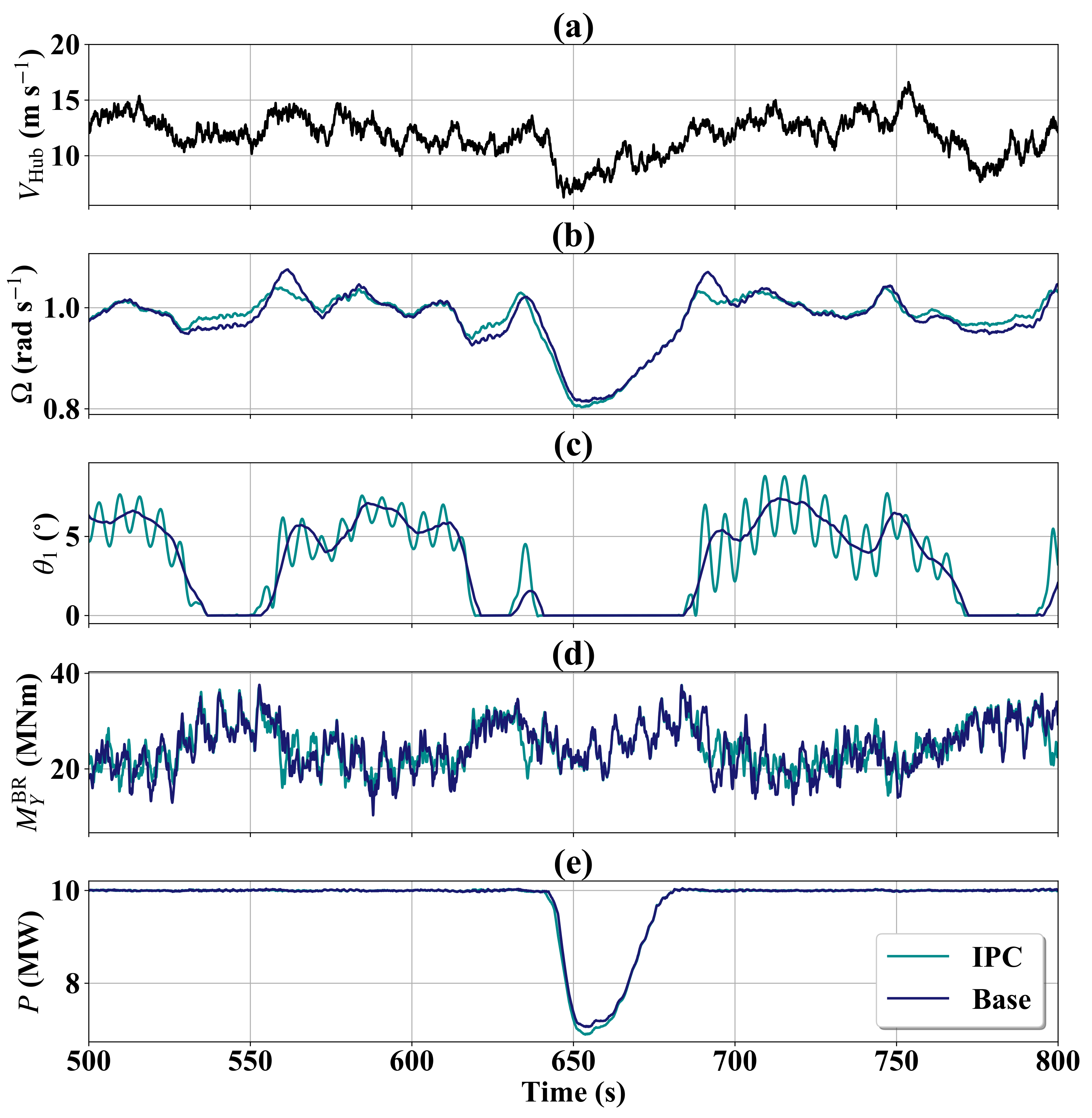
Figure 11 shows a selection of representative time series from a baseline simulation and a simulation with active IPC strategy. Both simulations use the TUB Controller with the same controller parameters. The baseline simulation uses the CPC strategy and the IPC simulation uses the CPC and IPC strategies. In this figure we can see the effect of the IPC strategy on the controller signals and on the
loads. From
Figure 11b,e it can be seen that the influence of the IPC strategy on
and
P is small. This is mainly due to the frequency separation between the CPC and IPC strategies.
Figure 11c shows the time series of
. We can clearly see the 1P oscillation of the IPC strategy on top of the CPC pitch signal. The load reducing effect of this strategy can be seen in
Figure 11d at around 700 s of simulation time. The 1P variation of
are clearly reduced due to the additional pitch actuation. The below-rated power limitation of the IPC strategy can be seen in
Figure 11c around 650 s of simulation time. When the mean pitch angle decreases to 0°, the amplitude of the IPC signal is also reduced 0° to maximize power capture.
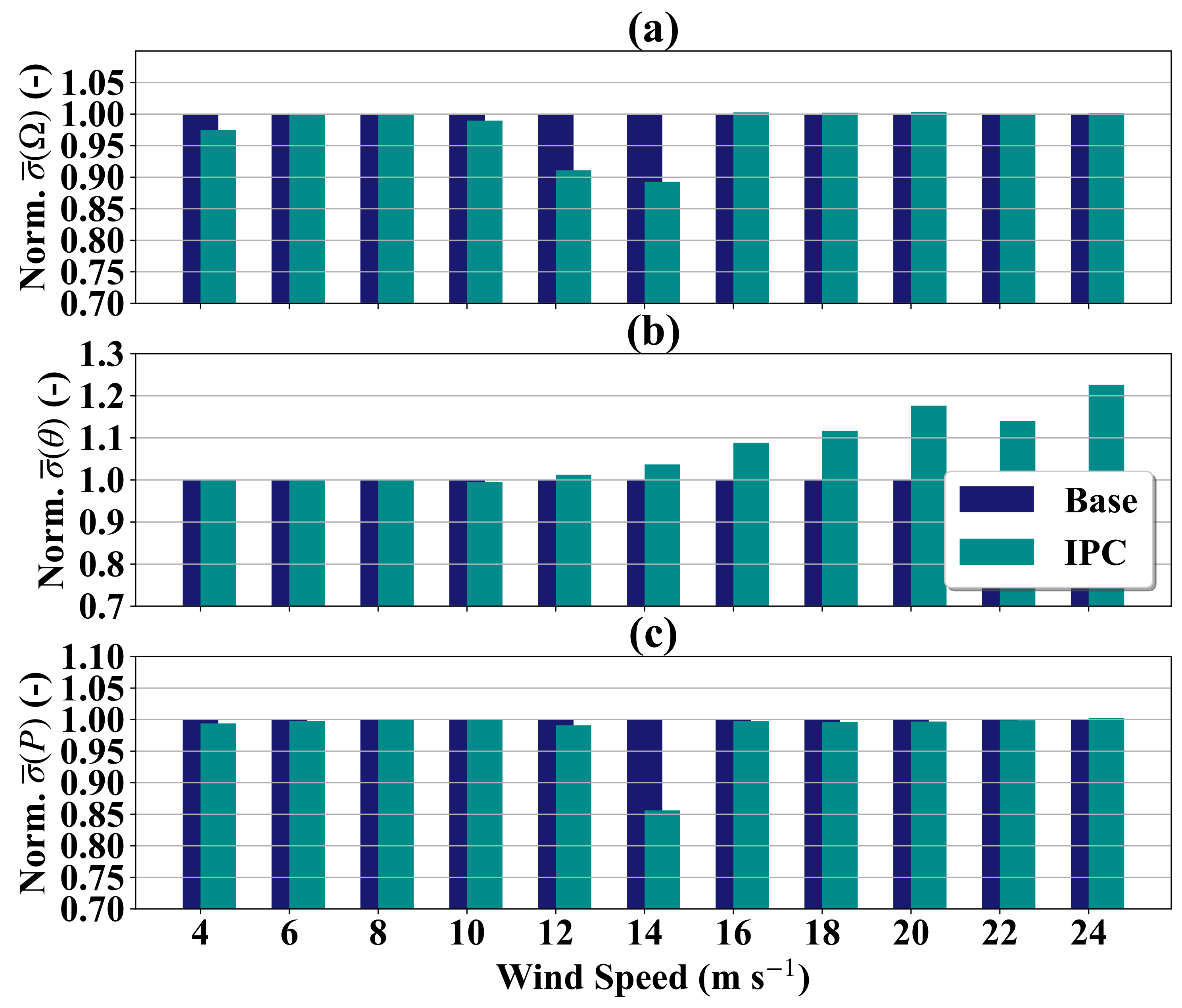
5.1.1. Controller Signals
The effect of the IPC strategy on the controller signals can be seen in
Figure 12. It shows the normalized averaged standard variations of
,
and
P respectively.
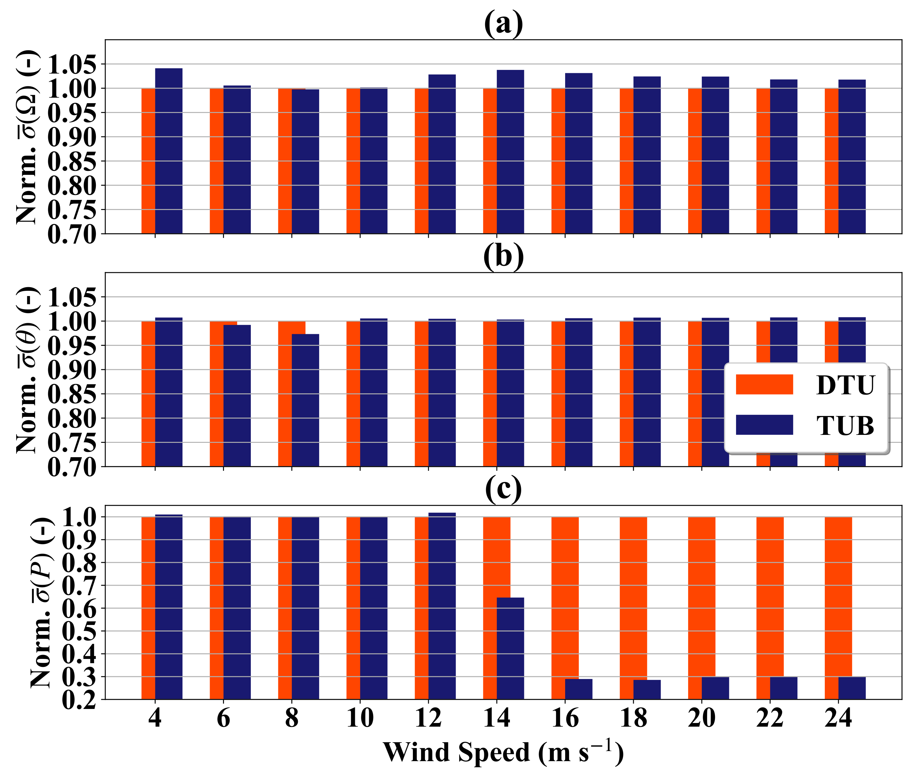
Figure 12a shows that the normalized
of the IPC strategy is practically 1 for all wind speed bins except the bins corresponding to 12 and 14 m/s average speed. There we see that
from the IPC simulations oscillates less than
from the CPC simulations. This can be understood if we look at
Figure 11b. The additional 1P fluctuation of
does influence the value of
by reducing slightly the sensitivity of the rotor to changes in the wind speed. This is particularly marked around rated wind, where the pitch angle is close to 0° and there are high angles of attack in the outer span of the blades. The latter lead to large values of lift forces and changes in the lift force due to pitching have an increased effect on rotor thrust and torque.
Figure 12b shows the normalized
vs. the wind speed bin. This is the controller signal that shows the largest differences. From 10 m/s onward, the value of
increases up to values larger than 1.2. It is this region where the IPC strategy starts to function. The increase in pitch activity from the IPC strategy is directly linked to the fact that the 1P fluctuation of
increases with increasing wind speed [
36].
Finally,
Figure 12c shows the normalized values of
. Here, there is almost no difference between the two strategies. The lower value in the IPC simulations seen in the wind speed bin of 14 m/s comes from the relatively small reference value of
for the CPC calculations. Because
P is fairly constant in above-rated wind simulations, differences in the drop of
P for temporarily low wind speeds (as seen in
Figure 11e) will have a large effect on the normalized
.
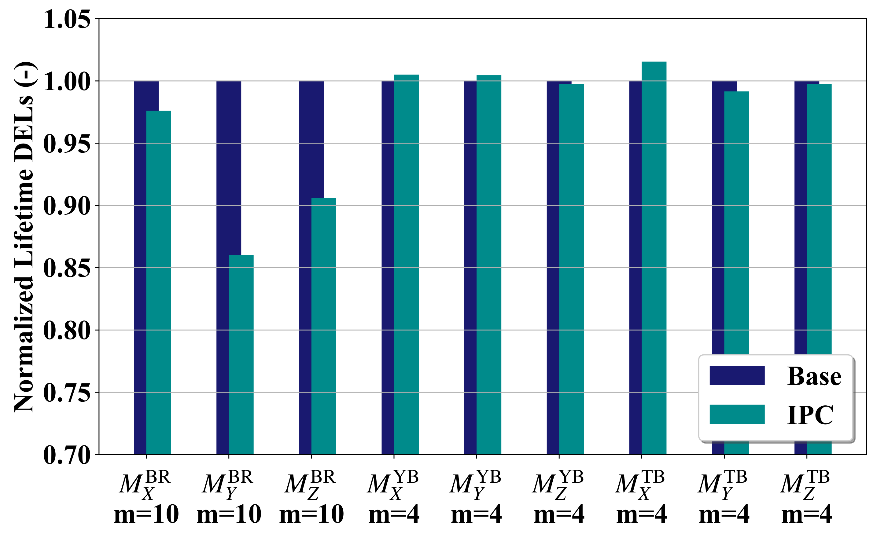
5.1.2. Fatigue Loads
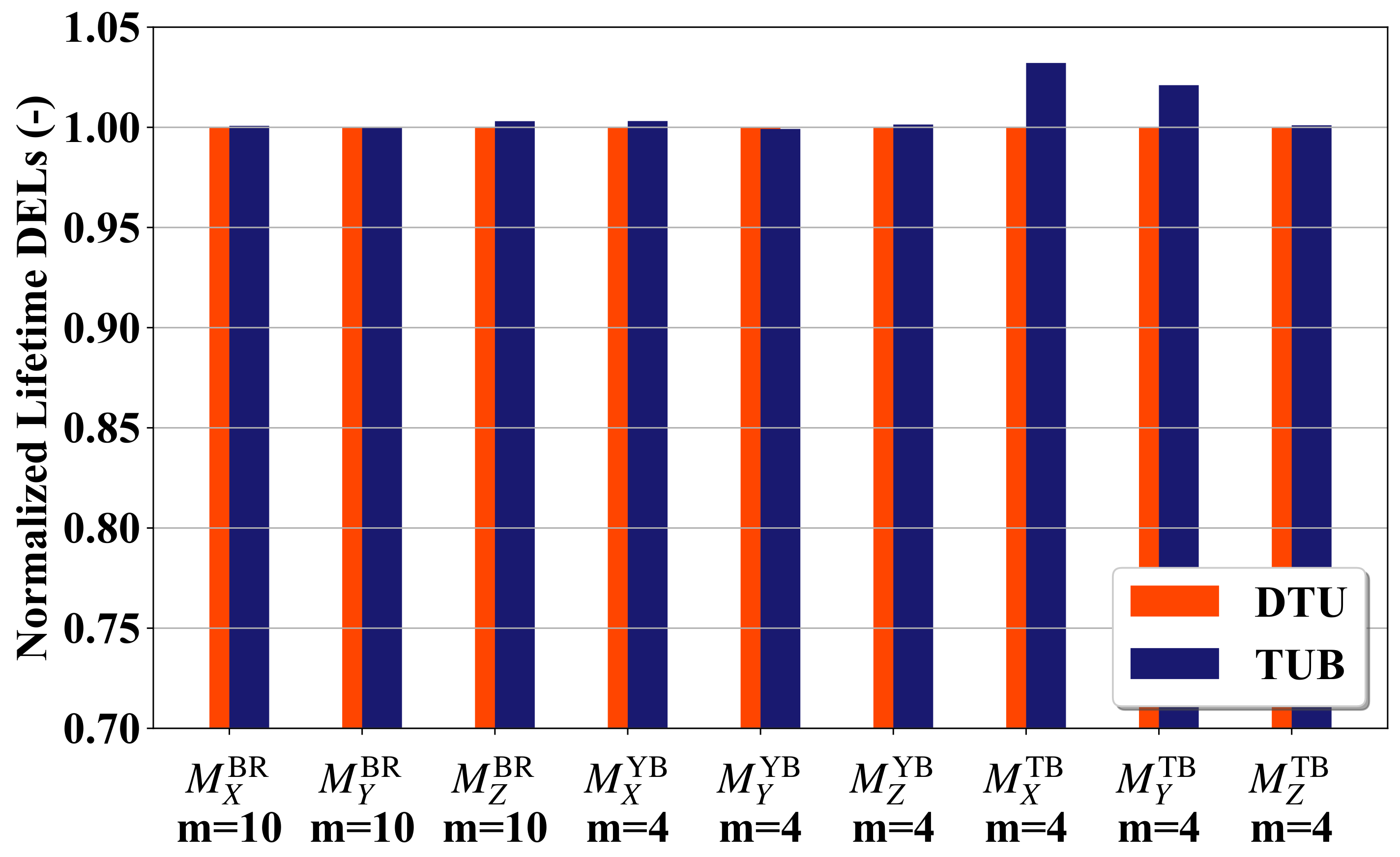
Figure 13 shows the normalized lifetime DELs of the simulations with the CPC and the IPC strategies. We can see that the main effect of the IPC strategy is to reduce the lifetime DELs of
and
by 14% and 9.4% respectively. There are also smaller effects on other load sensors. The lifetime DELs of
are 2.4% lower in the simulations with the IPC strategy compared to the CPC strategy. The load differences for these three sensors come directly from the IPC strategy. Since the strategy is minimizing the yaw and tilt moments of the rotor, it indirectly minimizes the load fluctuations of the individual blade root moments. These fluctuations arise from oscillations of the effective lift force on the individual blades. So, indirectly, the IPC strategy is also minimizing the fluctuation of the effective lift force on the individual blades. Although the out-of-plane component dominates in the lift force composition, there is also a smaller in-plane component. The former affects
and the latter
. Reducing the lift fluctuations also reduces the pitching moment oscillations and oscillations in the out-of-plane deflection of the blades. These two quantities directly affect
. So by reducing the lift force fluctuation, all three load sensors are affected.
The yaw bearing sensors are practically unaffected by the IPC strategy. This is due to the nature of our metric. The 1P based IPC strategy focuses on reducing the steady or slow varying yaw and tilt moments of the rotor. Our calculation of the DELs does not consider the means but only the ranges of the load cycles. A reduction of the load averages is therefore not captured by our metric. An IPC strategy that additionally targets the 2P load fluctuations would also reduce the yaw bearing DELs, ([
10,
20], (pp. 501–503)). The tower base lifetime DELs show that the IPC strategy also has a small impact on the tower fatigue loads. The IPC strategy increases the
DELs by 1.5% and decreases the
DELs by 0.9% compared to the CPC strategy.
6. Conclusions
This paper presented and detailed TUBCon, an advanced open-source wind turbine controller that includes pitch, torque and supervisory controllers. The controller can therefore be used to perform a complete load calculation according to industry standards. It is compatible with the common aeroelastic simulation codes including QBlade, which features the higher order LLFVW aerodynamic method in addition to a standard unsteady BEM aerodynamic model.
TUBCon was validated against an established turbine controller from the literature by comparing aeroelastic simulations of the DTU 10 MW RWT in steady and turbulent wind conditions. For steady wind conditions, the controllers show practically the same performance. For turbulent wind conditions, TUBCon shows a more aggressive constant power regulation. This reduces the mean standard deviation of the generator power for the above-rated wind bins by up to 70%, but increases the standard deviation of the rotor speed by up to 3.7%. This difference also affects the lifetime DELs of the tower base bending moments. The lifetime DELs of and are increased in the TUBCon simulations by 3% and 2% respectively.
We also investigated the advanced load reduction capabilities of TUBCon by comparing the performances of the IPC strategy against a baseline CPC strategy. This was done using QBlade’s LLFVW aerodynamic method, which is able to calculate the aerodynamic effects of a non-homogeneous induction field due to individual pitching more accurately compared to most BEM-based aerodynamic methods. The results show that the IPC strategy is able to reduce the lifetime DELs of and by 14% and 9.4% respectively when compared to the baseline simulations. This comes at the cost of increased pitch activity from the IPC controller. The normalized of the IPC strategy increase to values up to 22.6% higher than the values of the CPC strategy for wind speed bins above rated wind speed.
Future work will include further development of TUBCon to add new features such as tower vibration damping and rotor speed exclusion. It is also planned to add a fully featured trailing edge flap controller and the necessary features so that TUBCon can be used as a controller in offshore floating wind turbine simulations. Furthermore, the controller will be extended to include power curtailment and wake steering capabilities so that it can be used in conjunction with a wind farm controller. In addition, the effect of QBlade’s LLFVW aerodynamic model on advanced controller performance will be further analyzed by comparing the results from LLFVW-based simulations to more common BEM-based simulations and considering more DLC groups.


