
Generic EMT Model for Real-Time Simulation of Large Disturbances in 2 GW Offshore HVAC-HVDC Renewable Energy Hubs


 ,
,  ,
,  , and
, and
Abstract
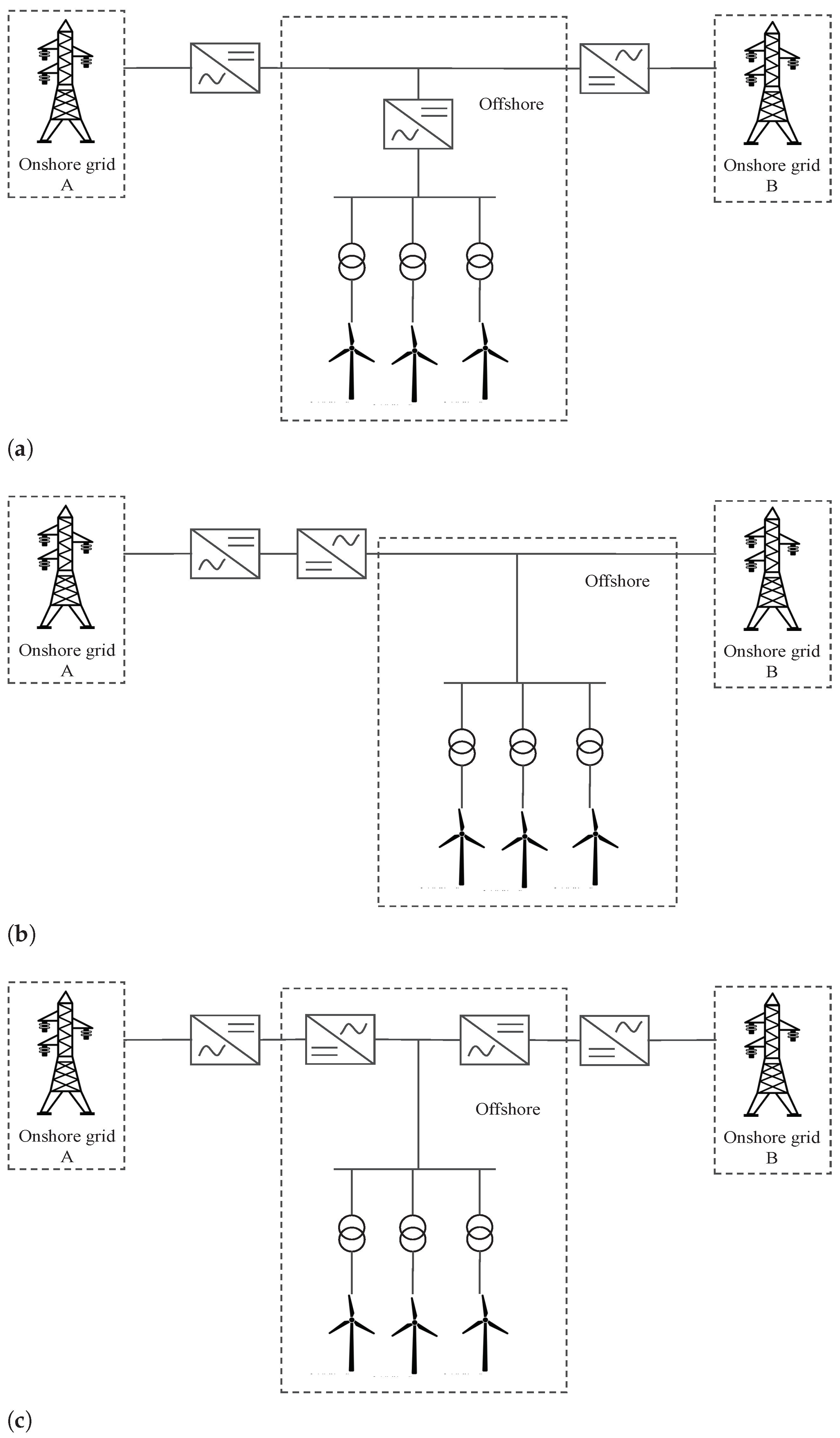
:1. Introduction
2. Defining the Layout for the 2 GW Offshore Network
2.1. Scaling of Single OWF Model for 2 GW Offshore Network
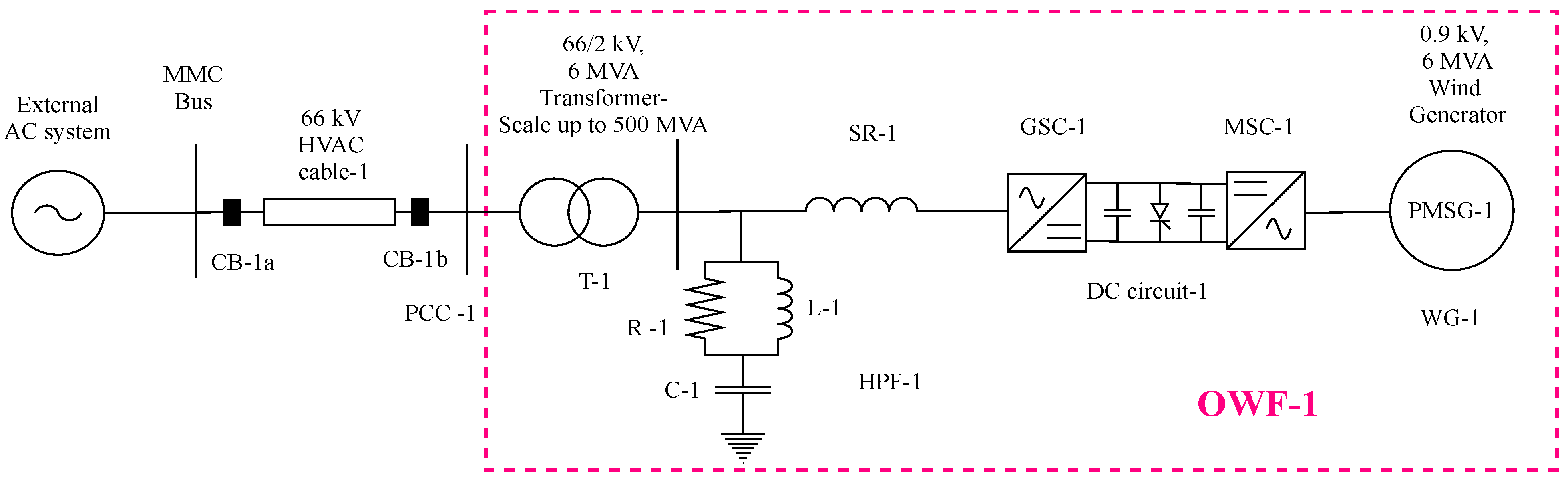
- The aggregated OWF model in [12] provides a generation of ∼700 MW. The first step involves reducing this generation to ∼500 MW, because there are four planned OWFs. This is achieved by reducing the number of parallel WG units from 116 (116 × 6 MW = 696 MW) to 83 (83 × 6 MW = 498 MW), which is done by changing the scaling factor at the OWF transformer. Thus, OWF generates approximately ∼500 MW, as shown in Figure 2.
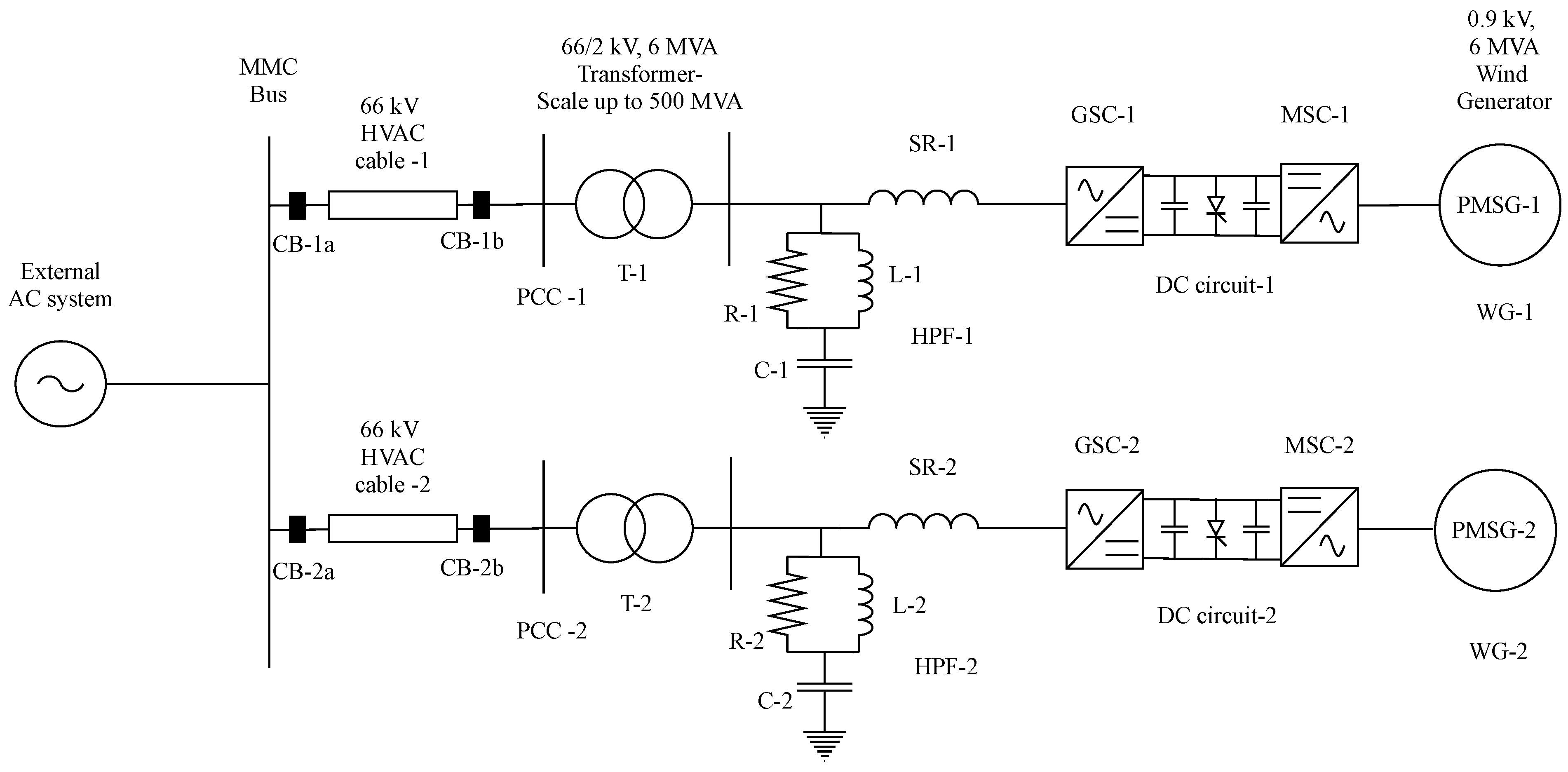
- The second step involves the connection of two OWFs in parallel to the external AC system in a modular approach. This allows for the generation of 1 GW of power, as depicted in Figure 3. All control structures incorporated in OWF-1 are replicated for OWF-2.
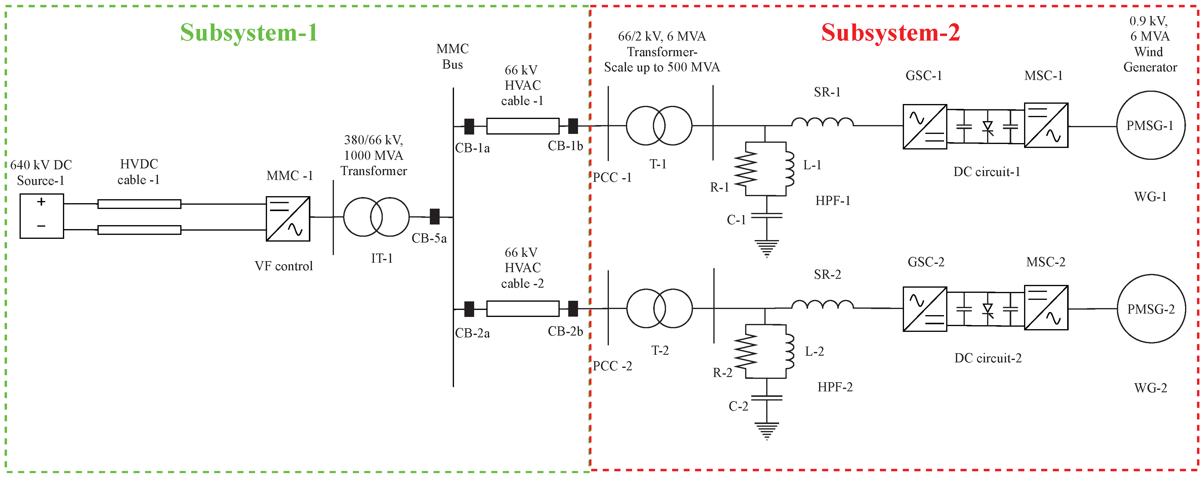
- In the third step, the external AC system is replaced by an offshore converter station, consisting of the average EMT model of MMC (MMC-1) and the interface transformer (IT-1), which is available in the CIGRE B4 DC Grid Test System [14]. The same is depicted in Figure 4. As the final layout network would be extensive, it is required to split the network into subsystems. The splitting into two subsystems is performed in this step. The offshore converter station is modelled in subsystem-1, and the OWFs are modelled in subsystem-2. MMC-1 is designed to operate in V/F control (or grid forming control), which is explained at the end of this section.
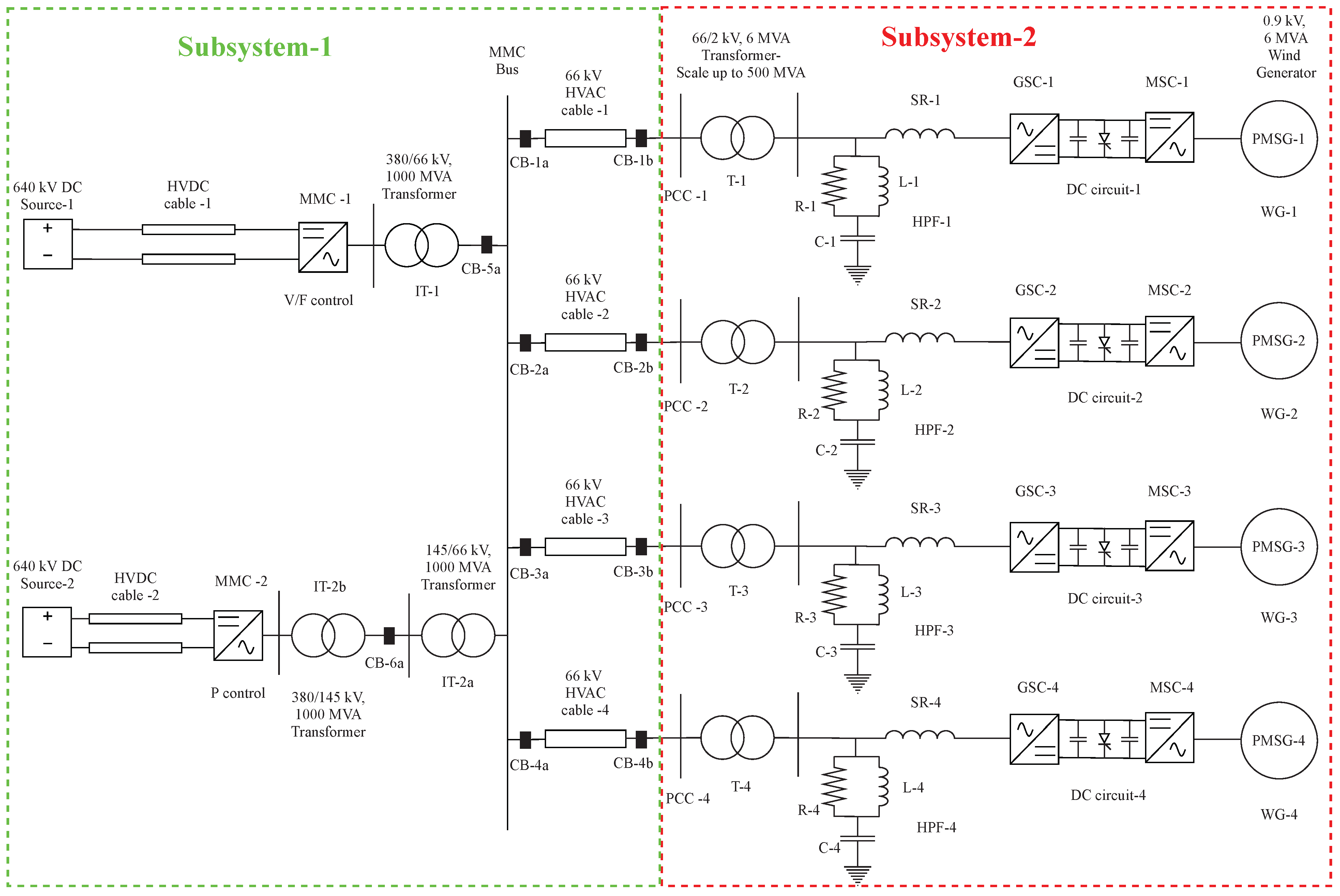
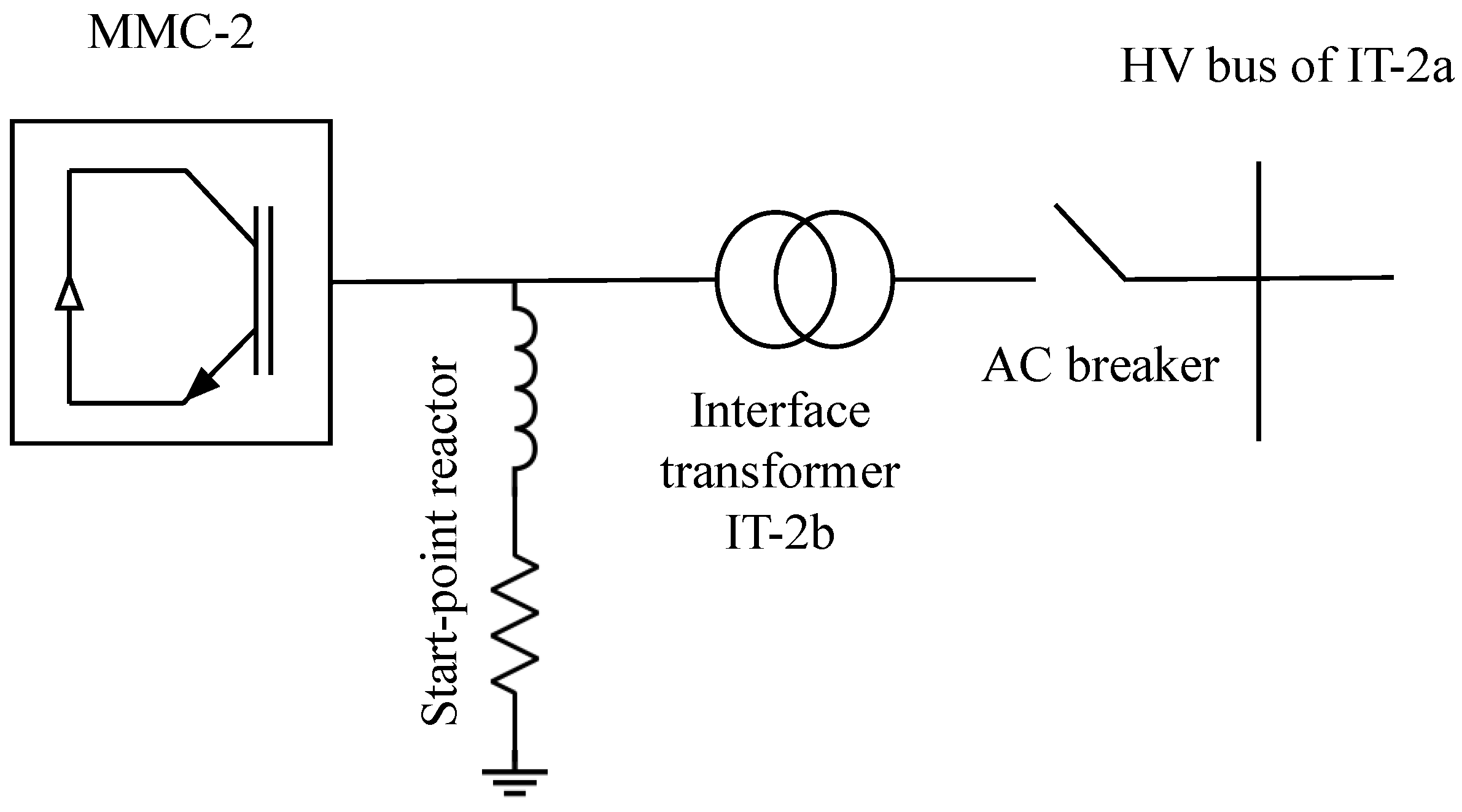
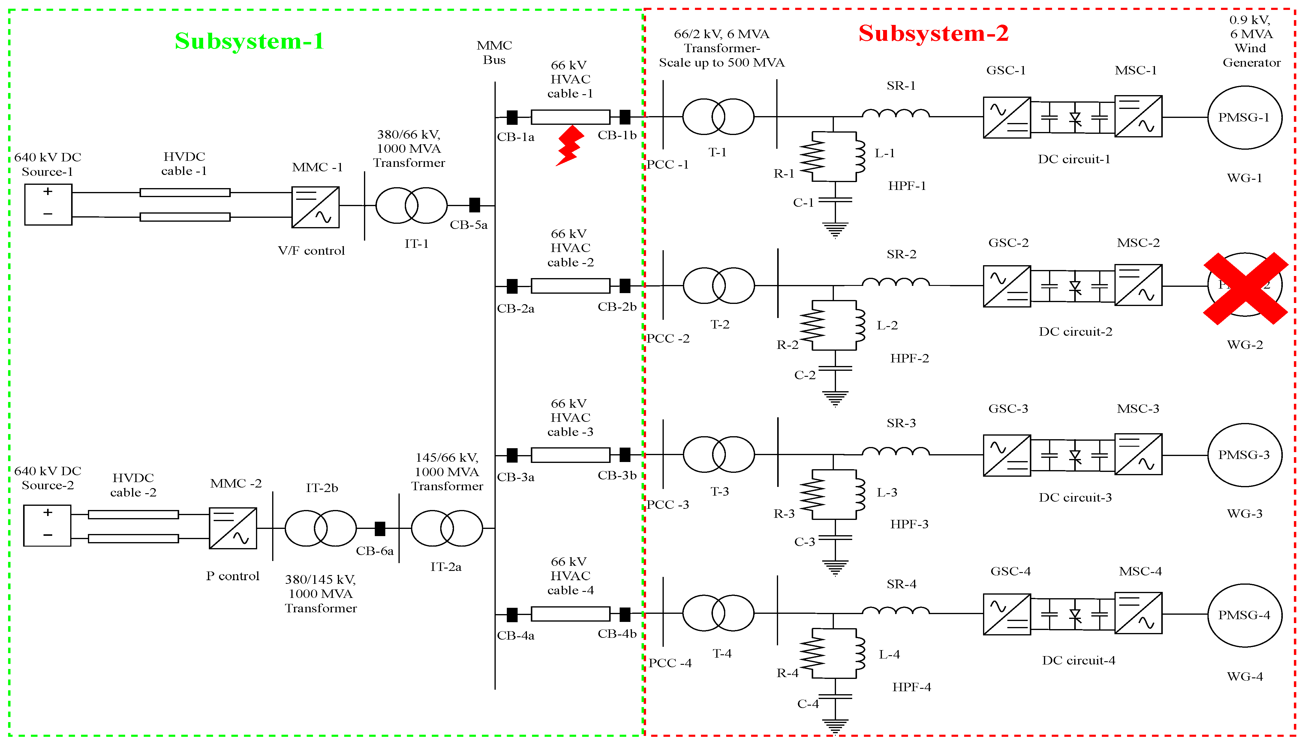
- The final step involves parallel connection of the two more OWF models (OWF-3 and OWF-4), generating ∼500 MW each, using modular approach. Additionally, another offshore converter station, consisting of a similar average EMT model of MMC (MMC-2) and two interface transformers (IT-2a and IT-2b), is connected in parallel to the previous converter station. The need for two interface transformers in MMC-2 bus is explained in the following sections of the paper. Therefore, the final layout shown in Figure 5 represents a total of 2 GW offshore wind power transmission.
3. Layout of 2 GW, 66 kV HVAC Offshore Network in RSCAD
3.1. Aggregated OWF
3.2. HVAC Cables
3.3. Offshore Converter Stations
3.3.1. Interface Transformers
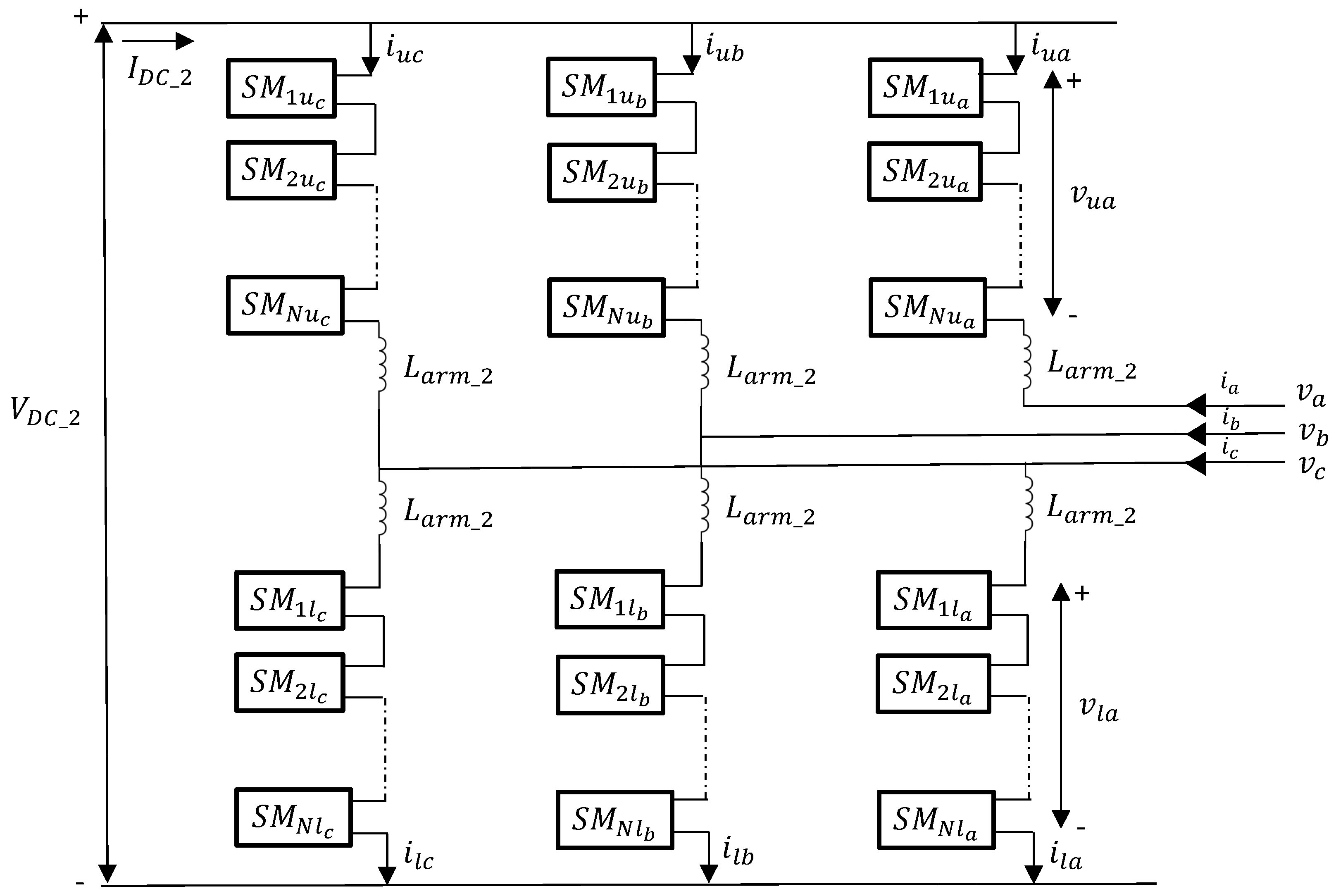
3.3.2. Modular Multilevel Converters (MMCs)
3.4. HVDC Cables
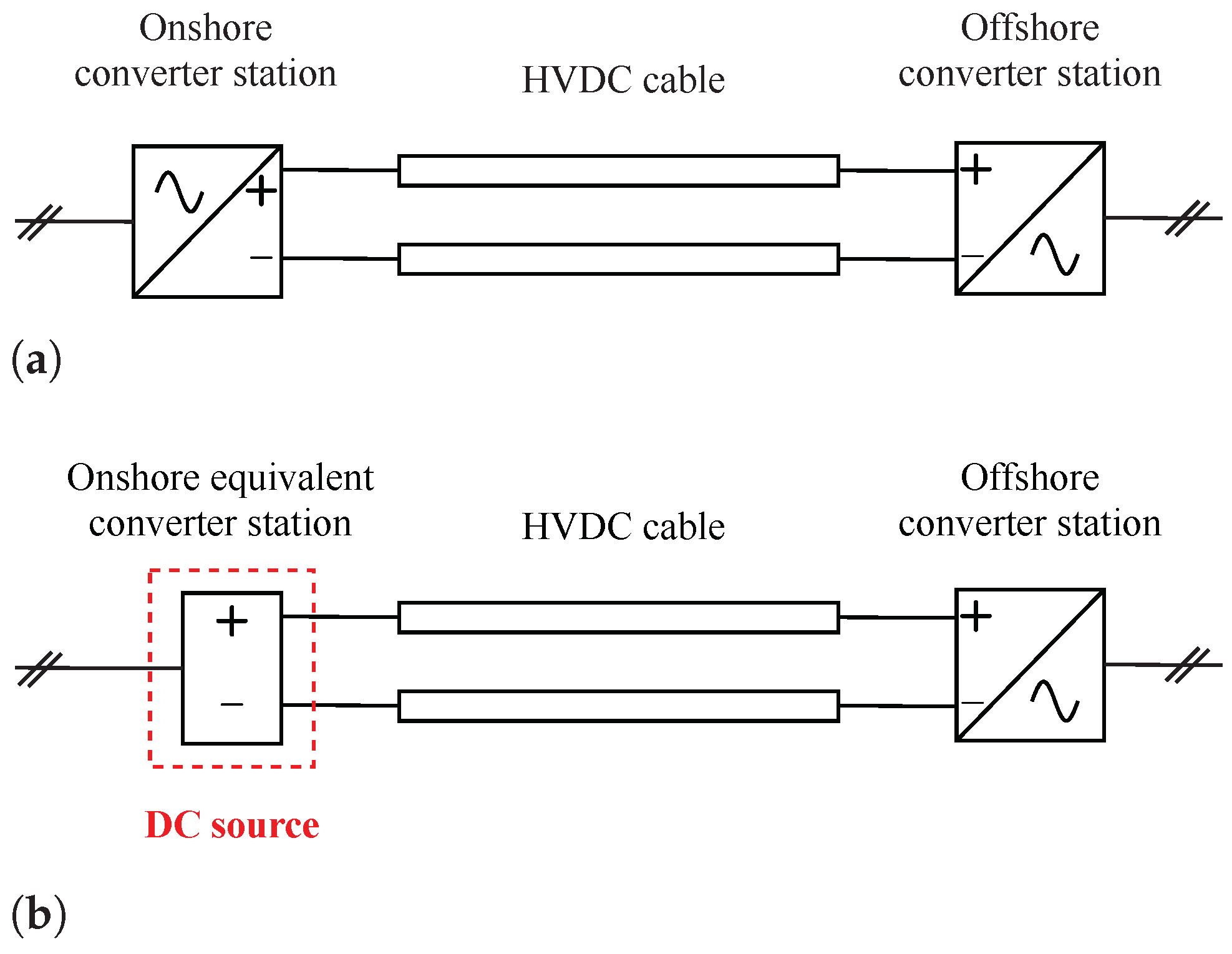
3.5. Onshore Equivalent Converter Stations
4. Control Structures
4.1. DVC
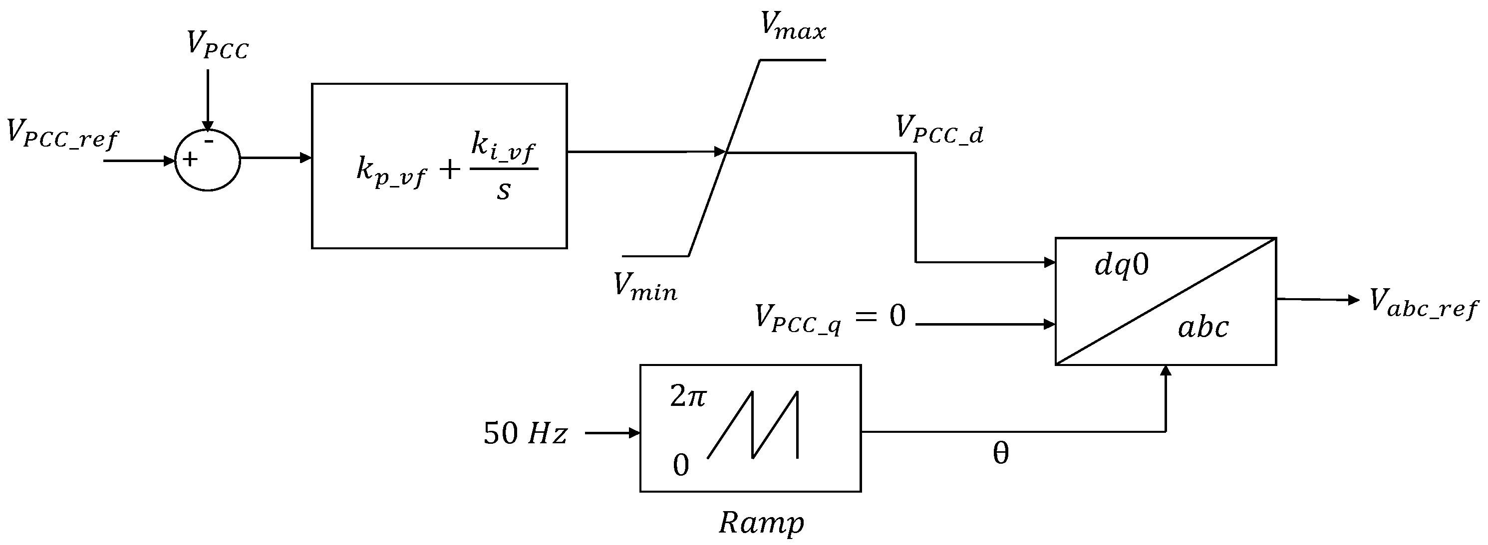
4.2. Island Mode Control
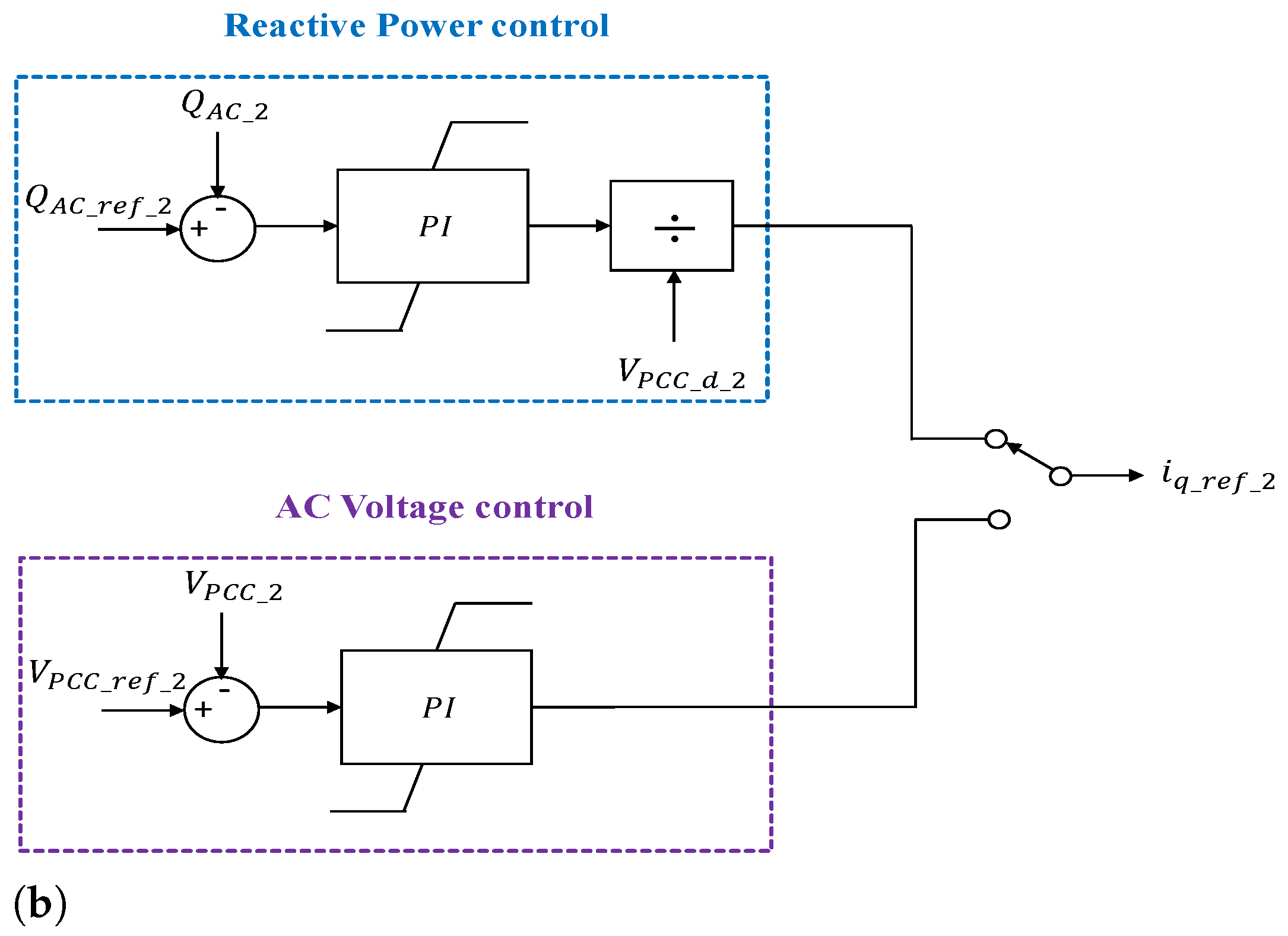
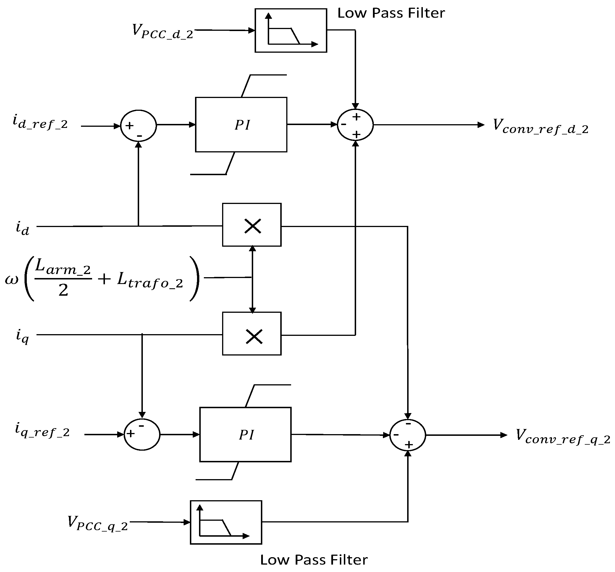
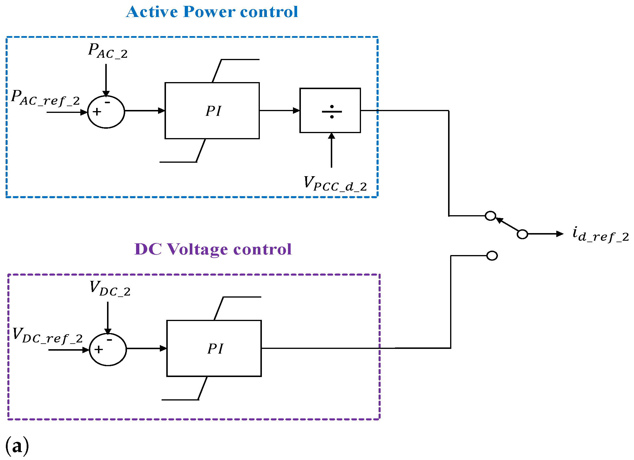
4.3. Non-Island Mode Control
5. Numerical Simulations in RSCAD
5.1. General Settings, Control Modes and Pre-Set Conditions
- MMC-1:
- −
- Islanded mode operation (V/F control)
- −
- AC voltage control, = 1 p.u. (Reference AC voltage)
- MMC-2:
- −
- Non-islanded mode operation
- −
- Active power control, = 0 (No power flow through MMC-2 in the initial conditions)
- Network:
- −
- Circuit breakers (CB-1a, CB-1b, CB-2a, CB-2b, CB-3a, CB-3b, CB-4a, CB-4b, CB-5a and CB-6a) in open condition
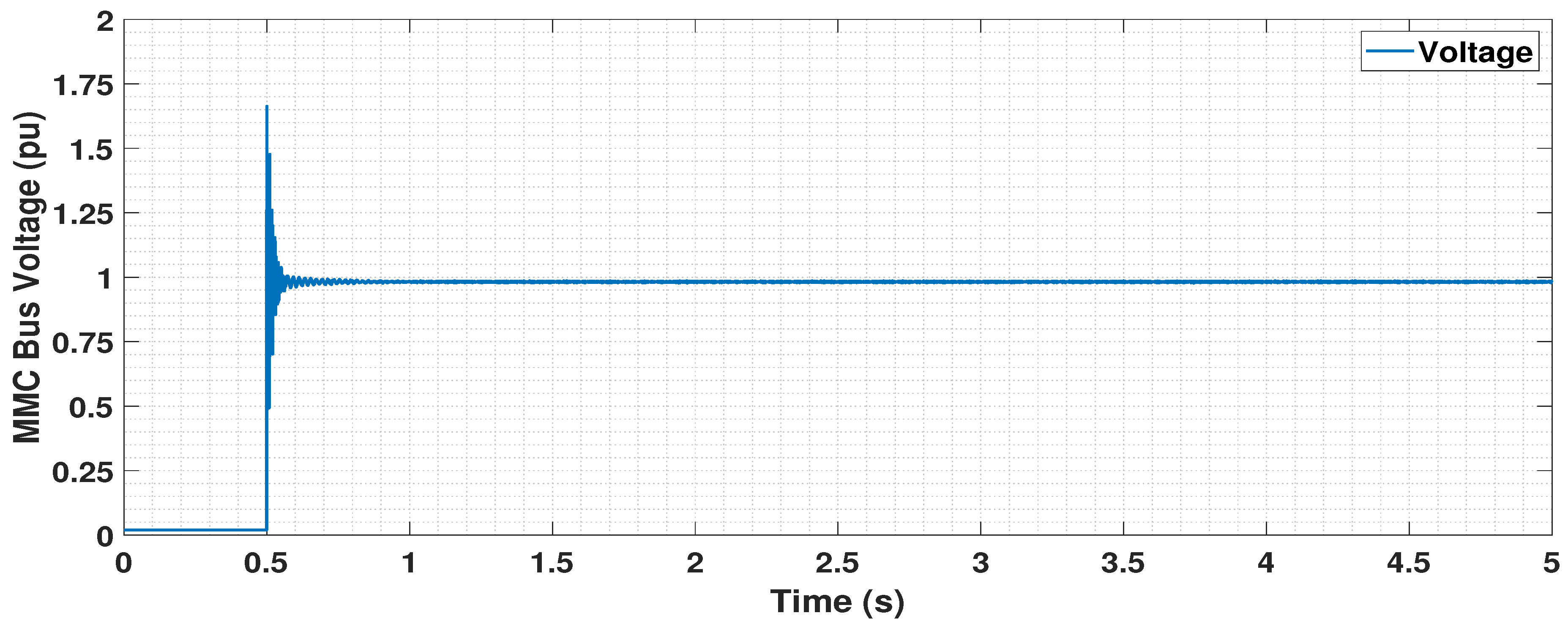
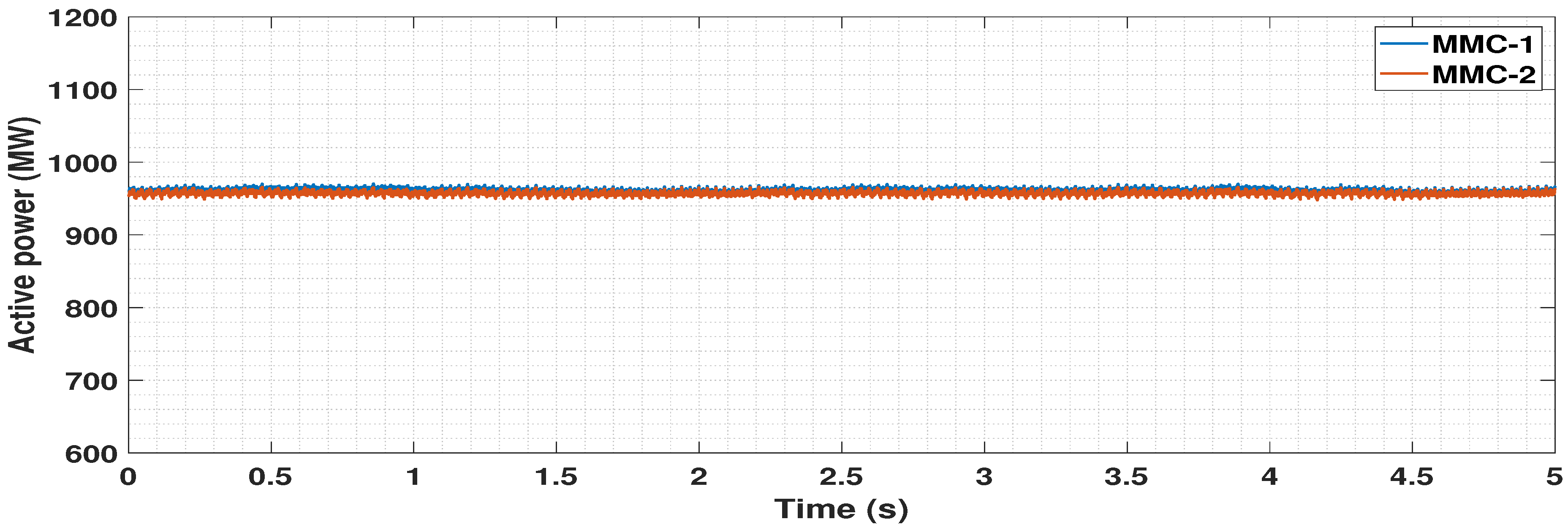
5.2. Synchronization of the Offshore Converter Stations
5.3. Energization of the HVAC Cables and OWFs
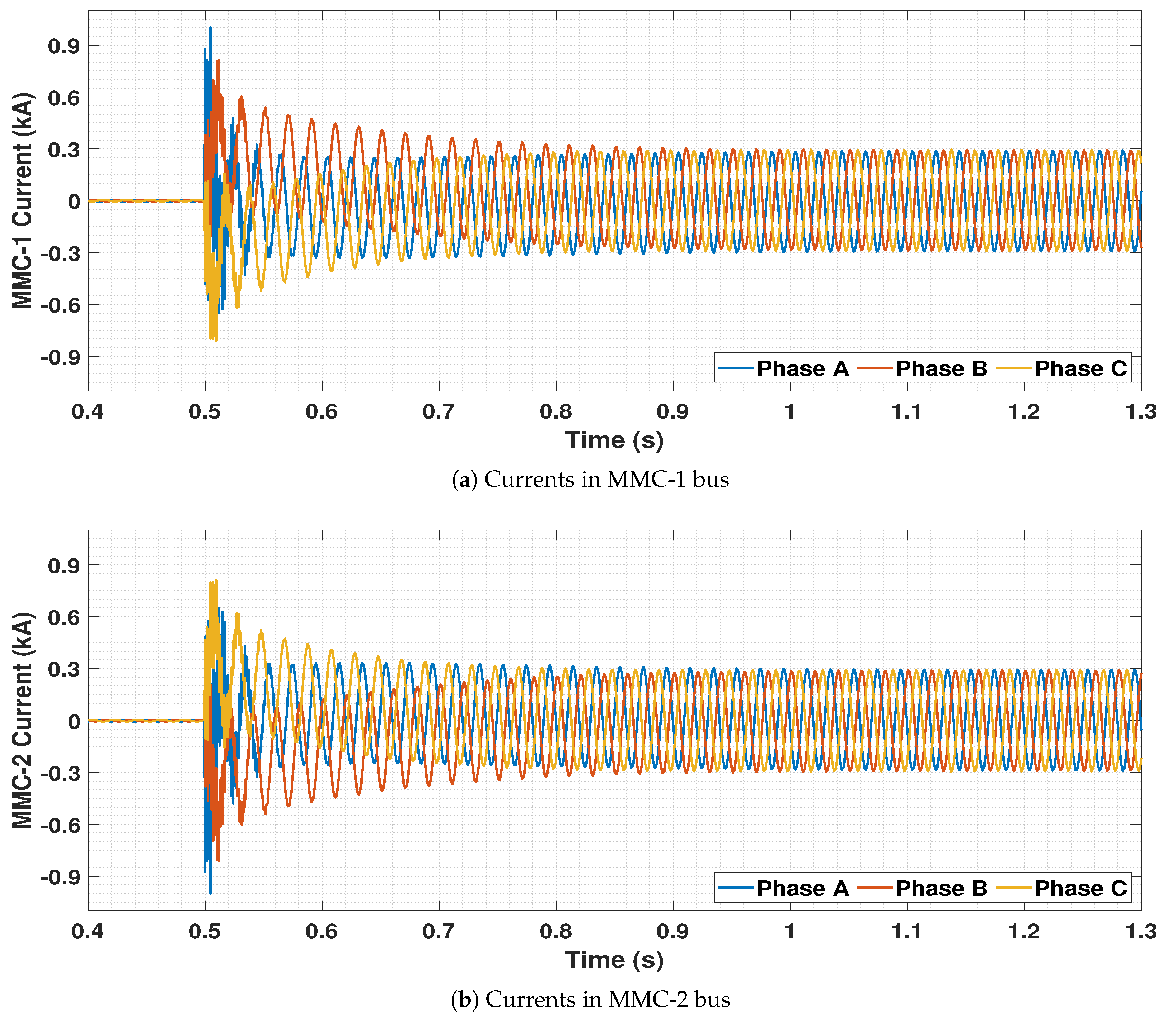
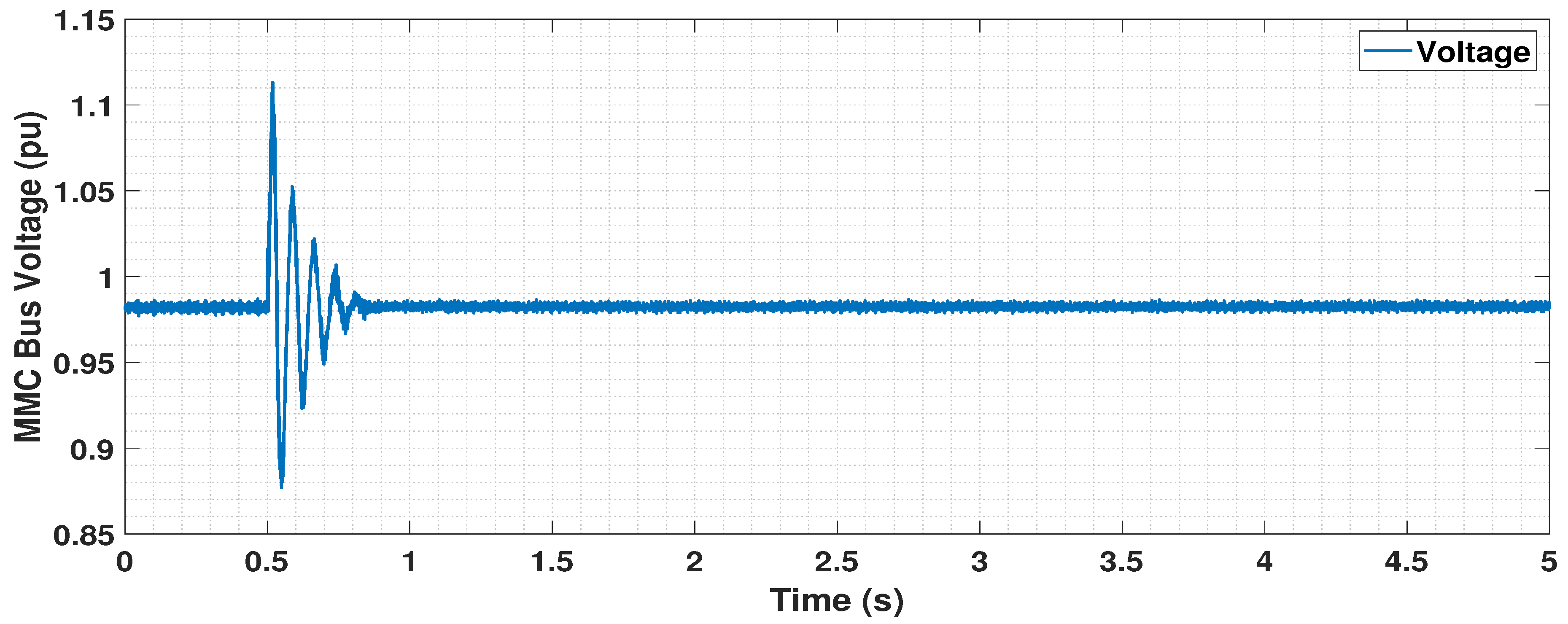
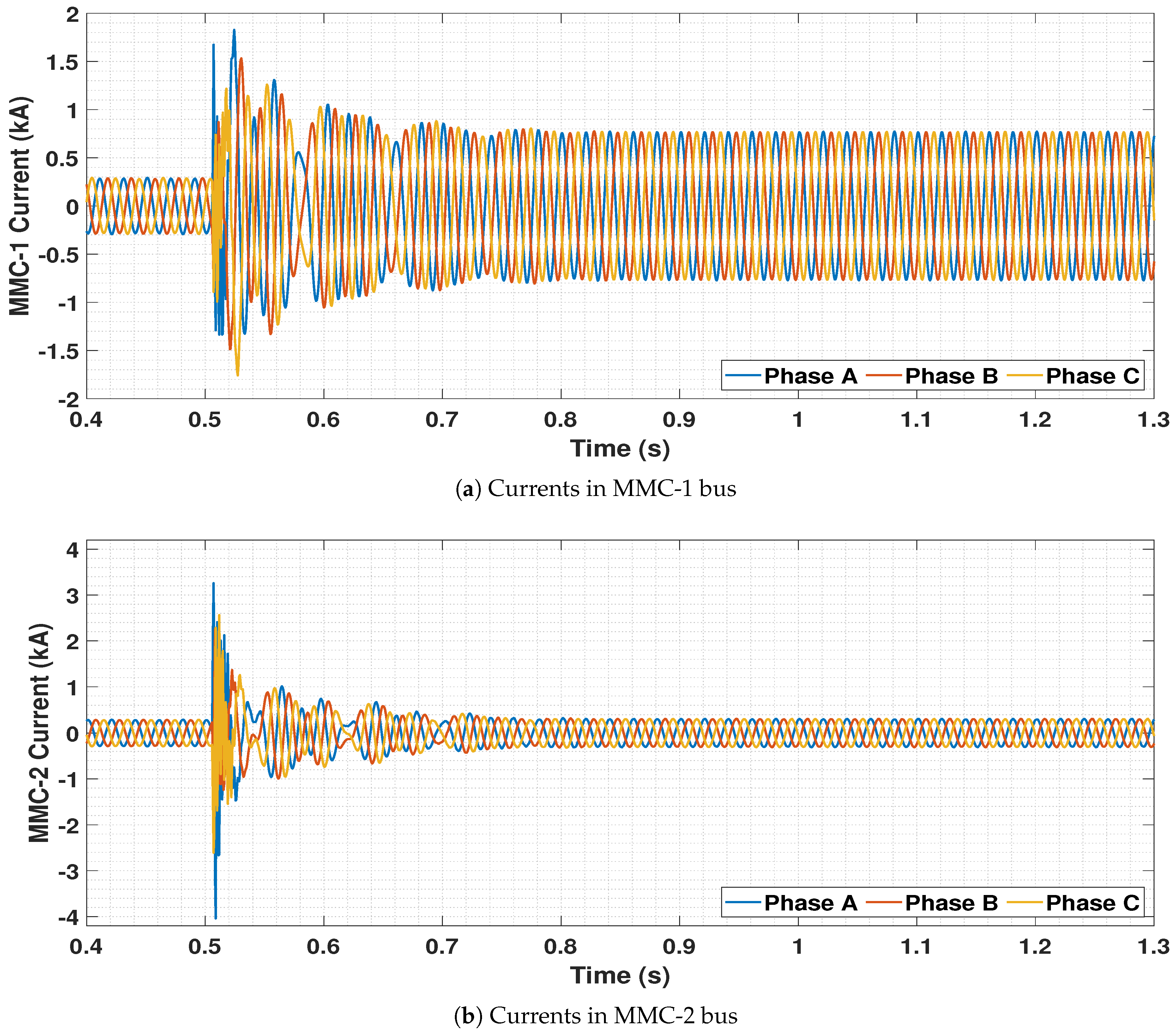
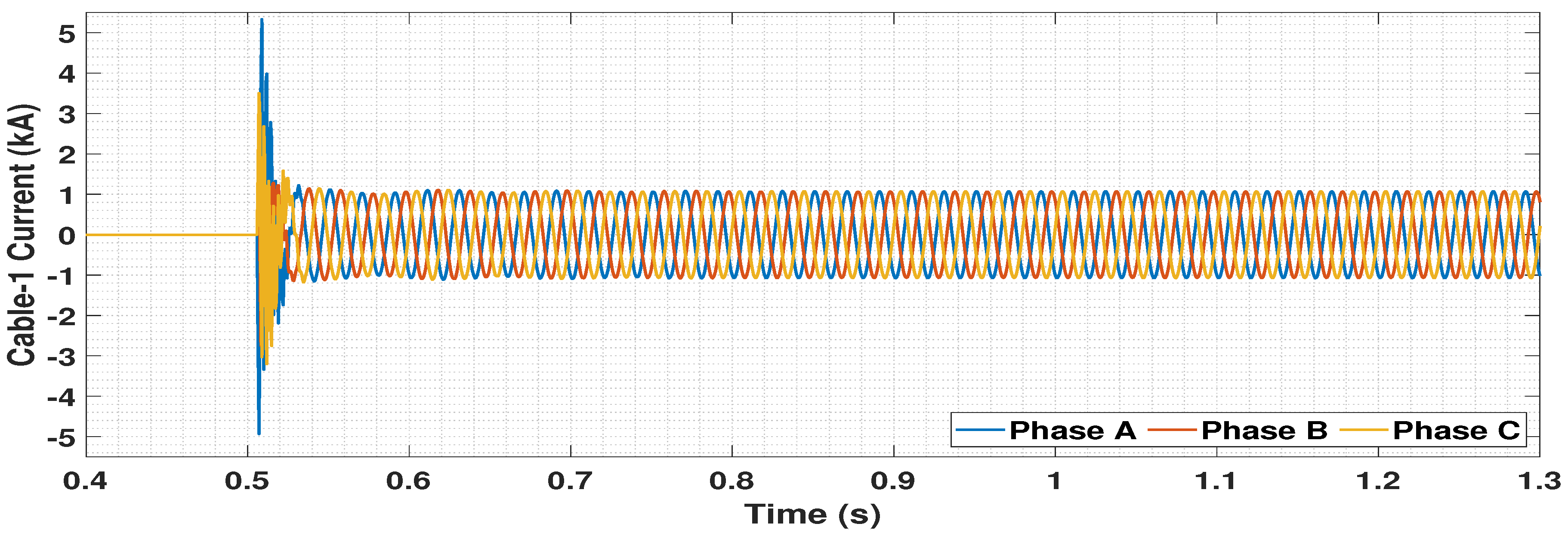
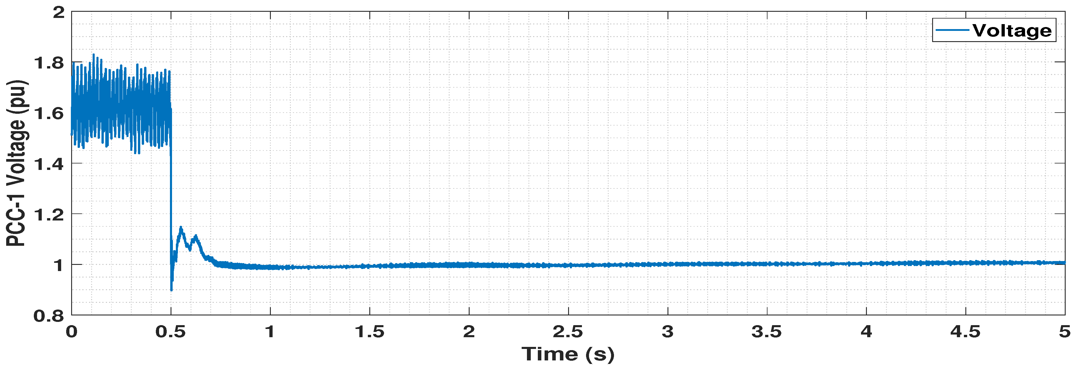
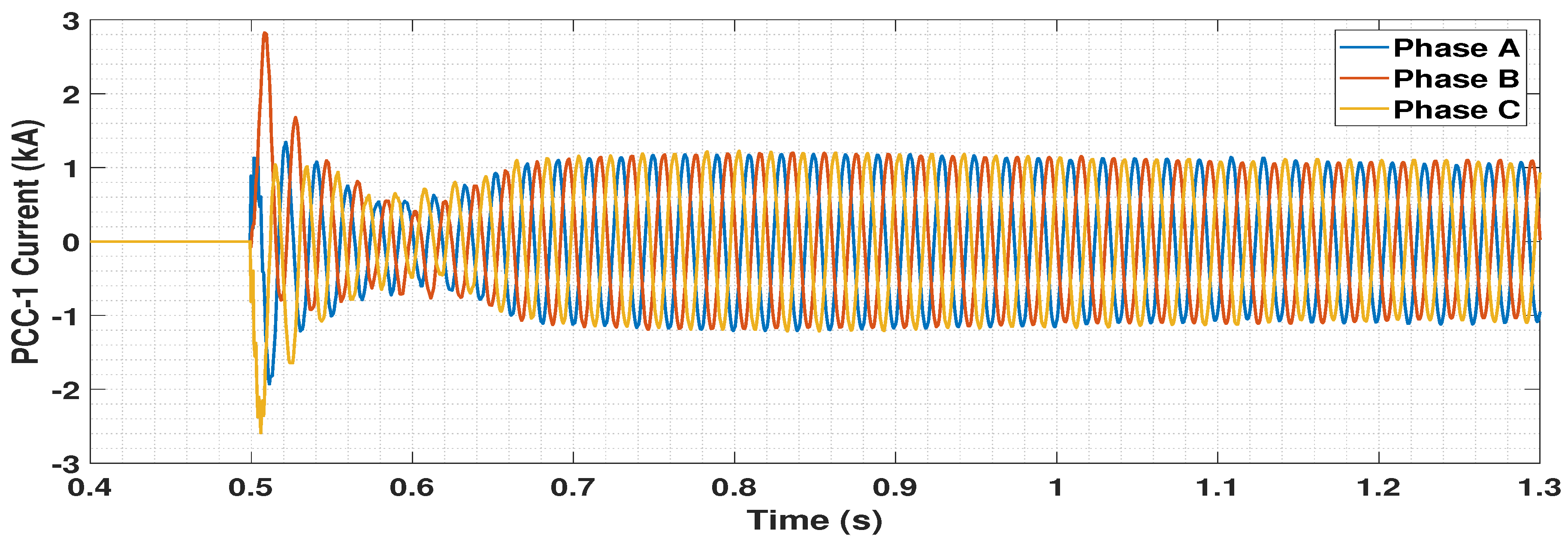
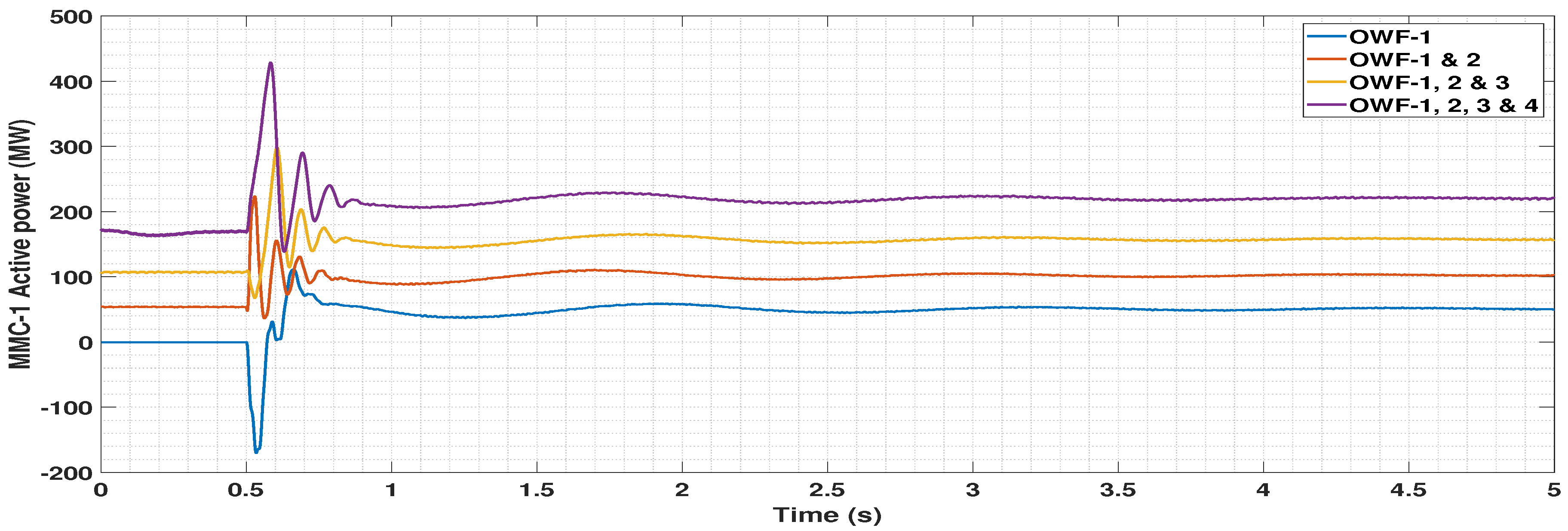
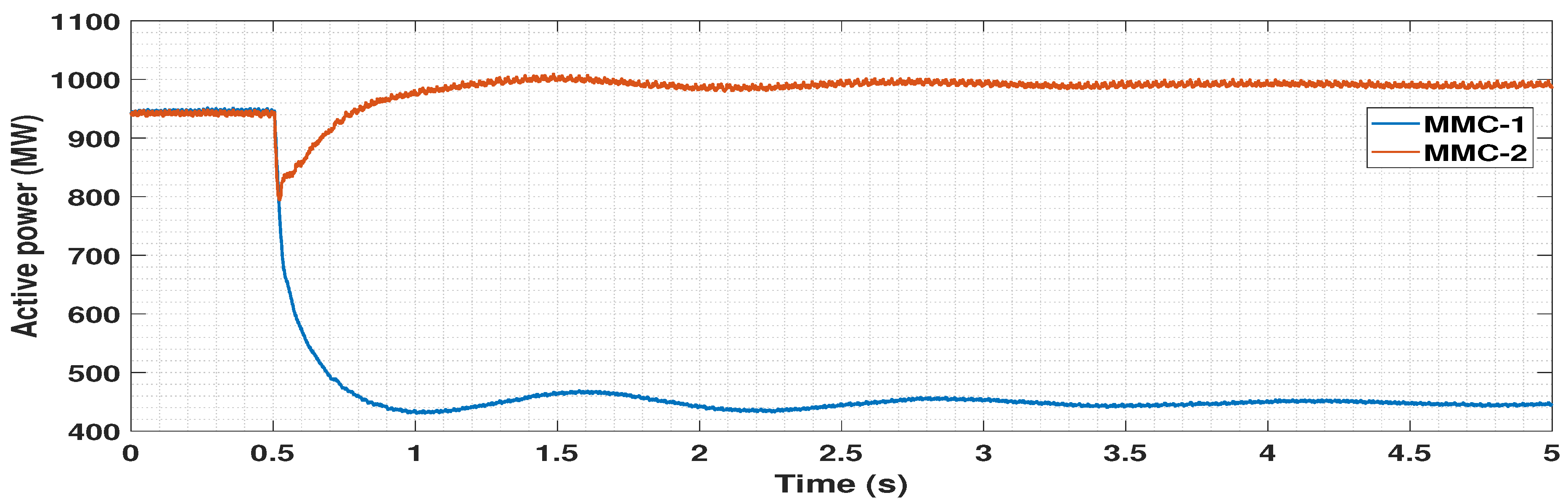
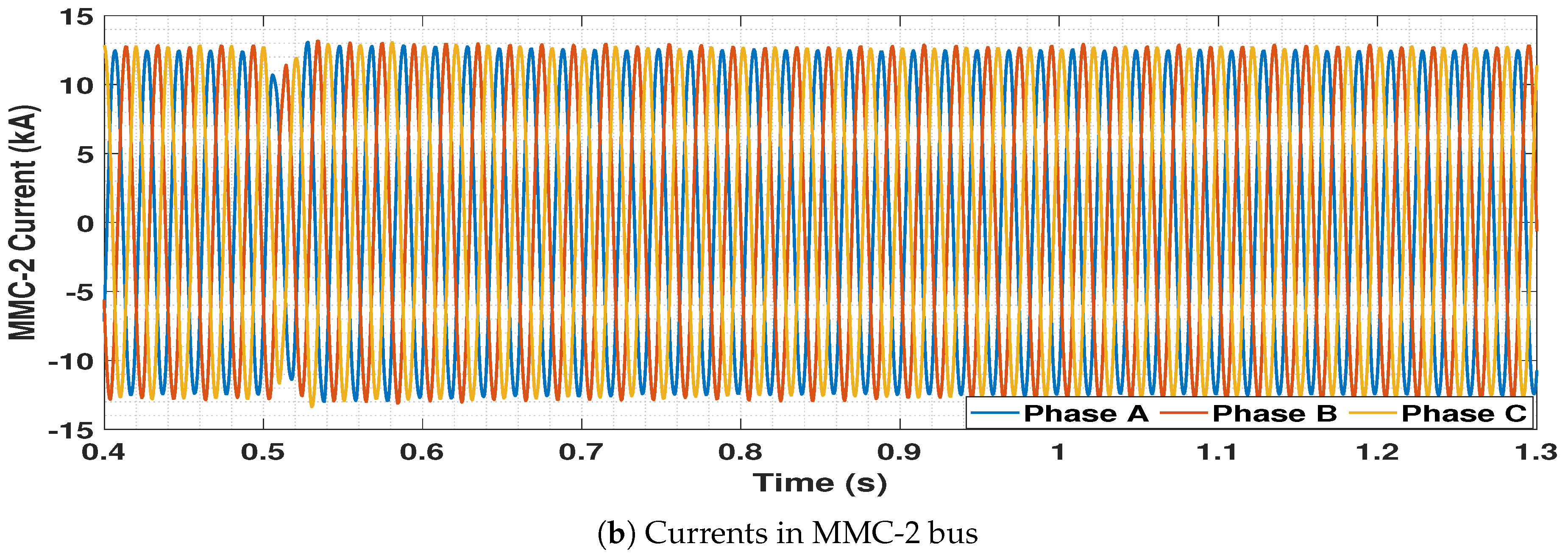
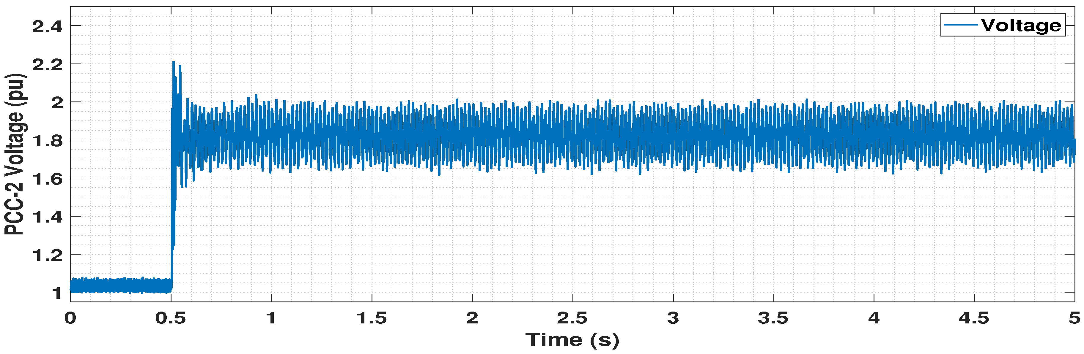
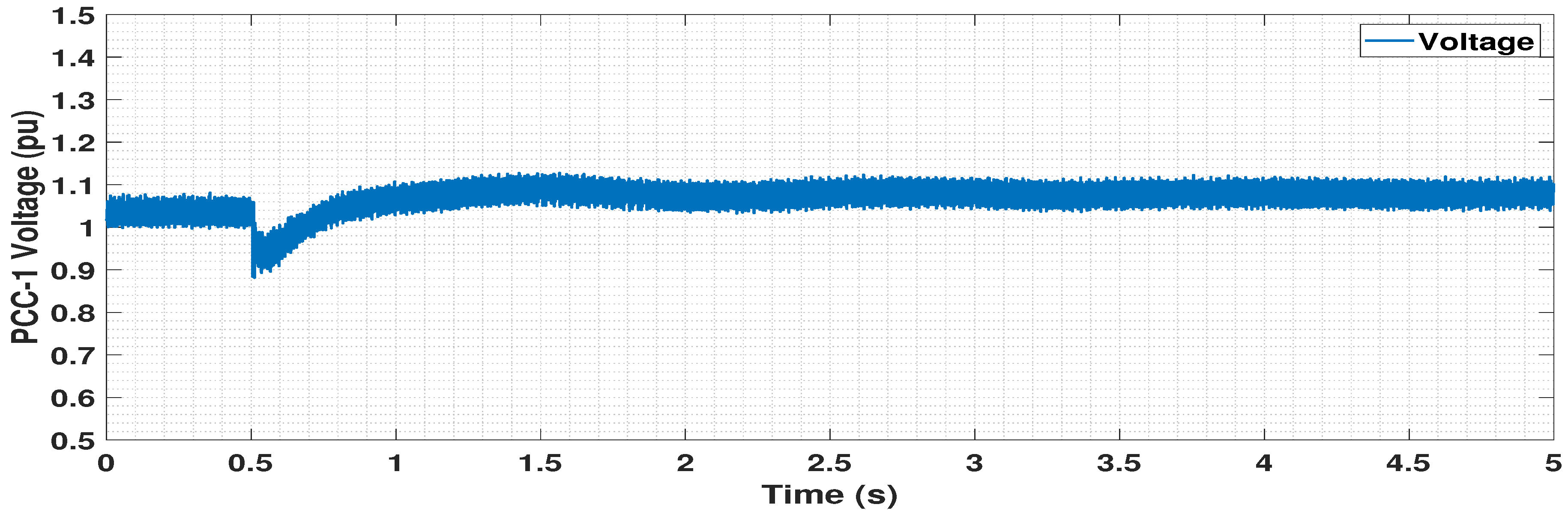
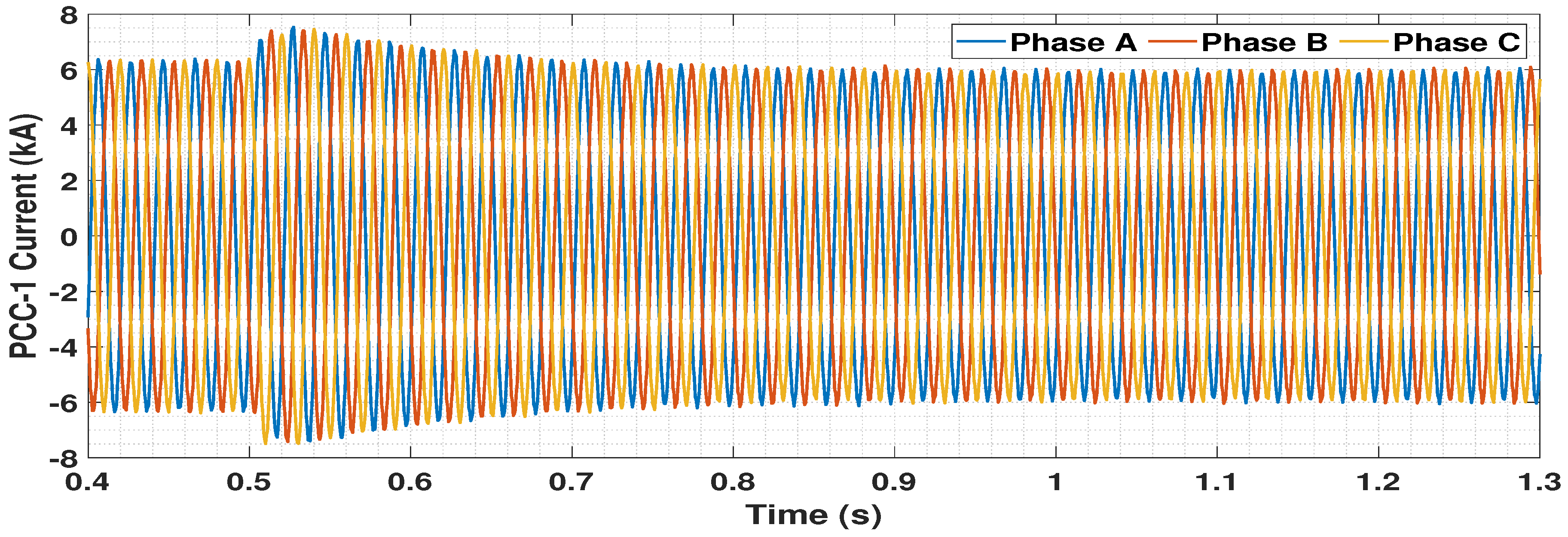
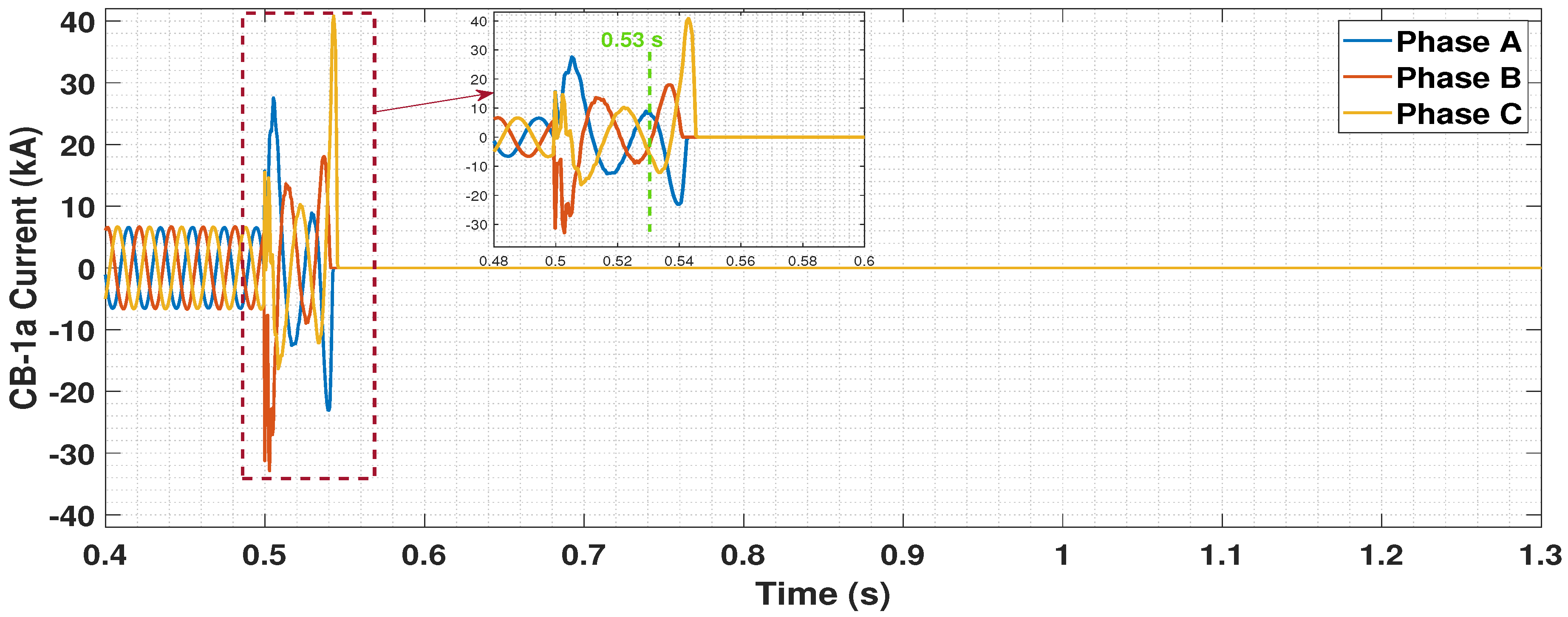
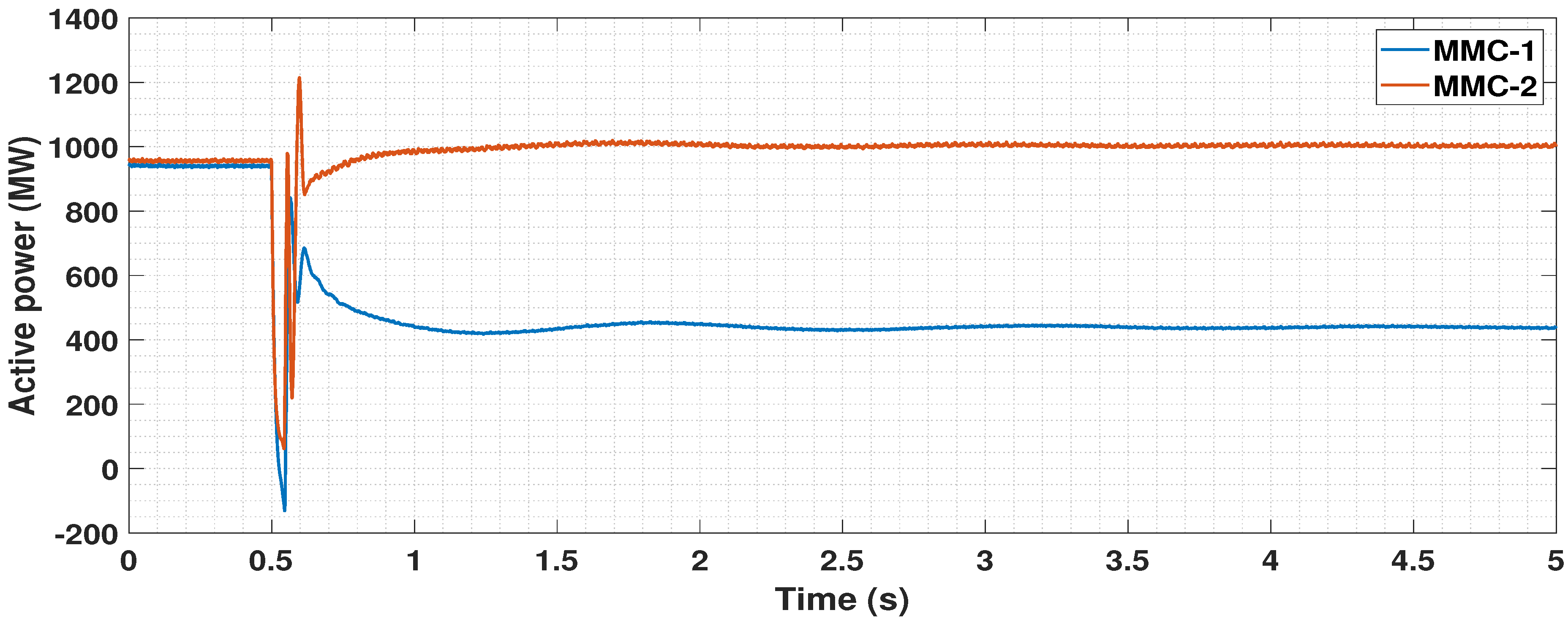
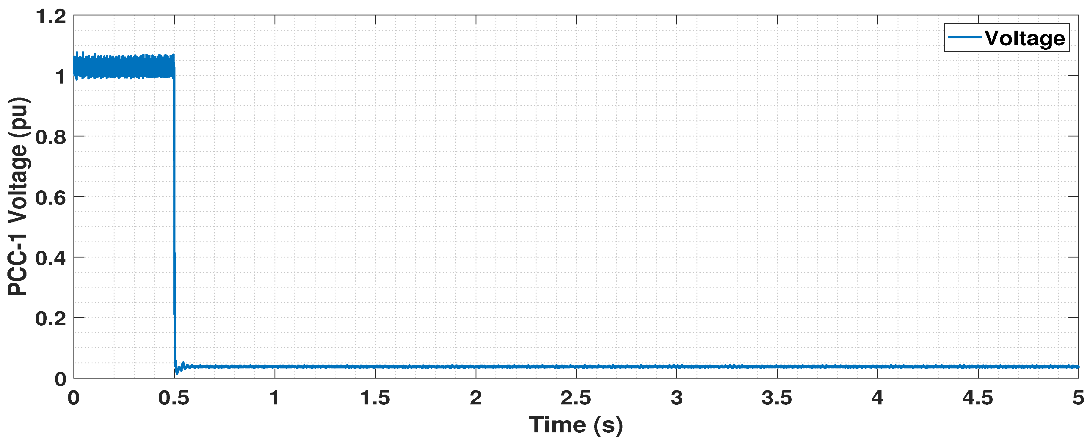
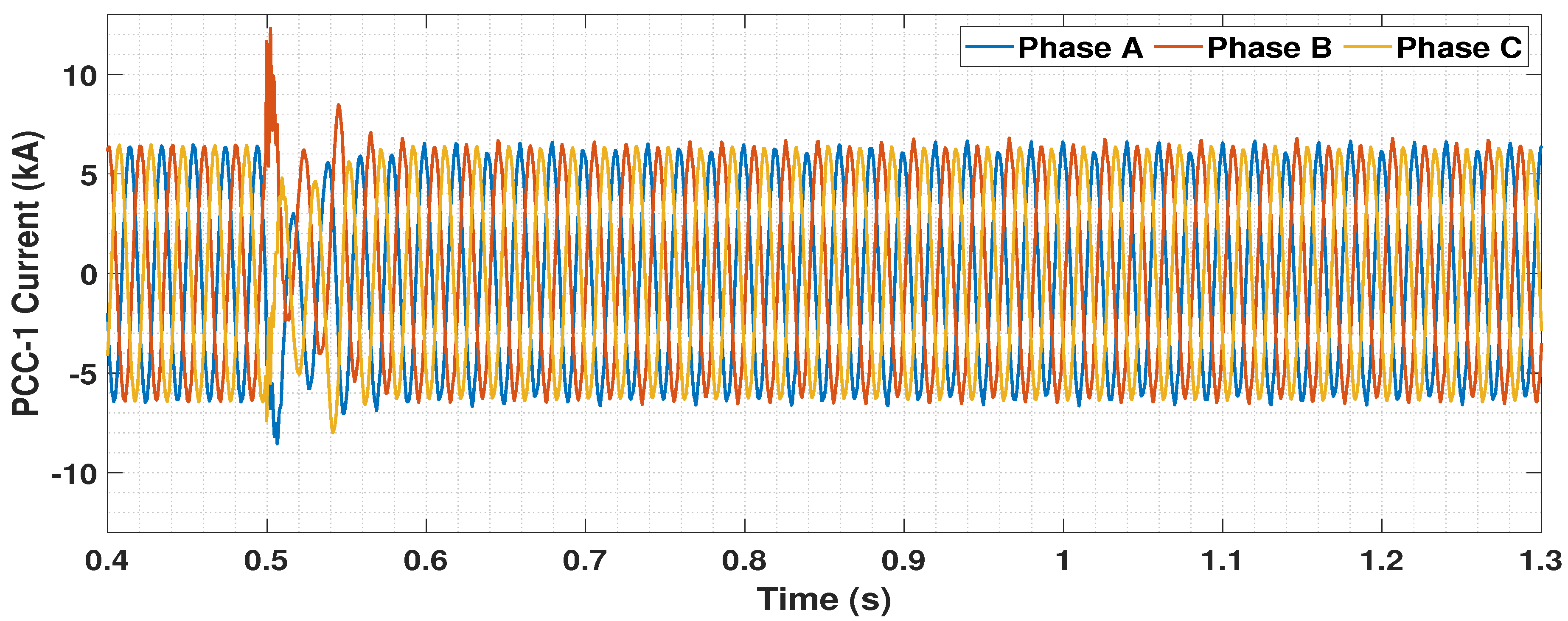
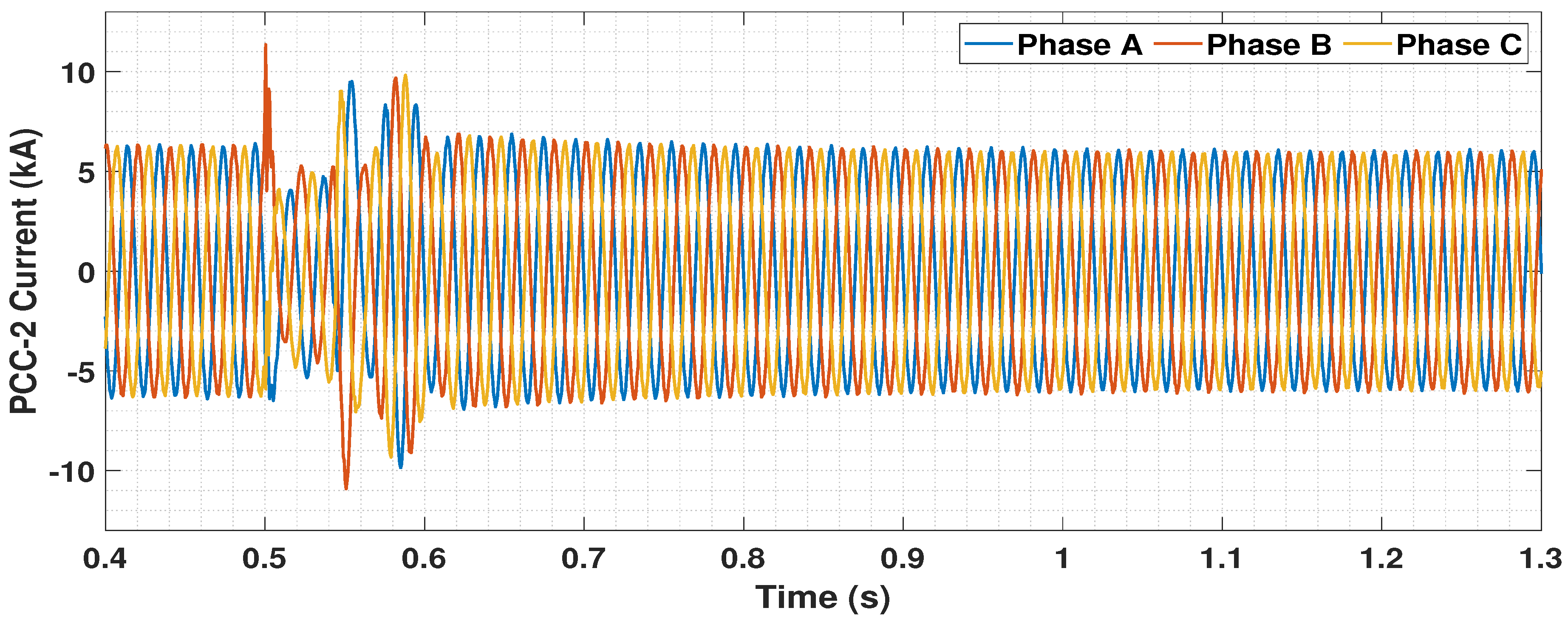
5.4. Dynamic Performance Analysis
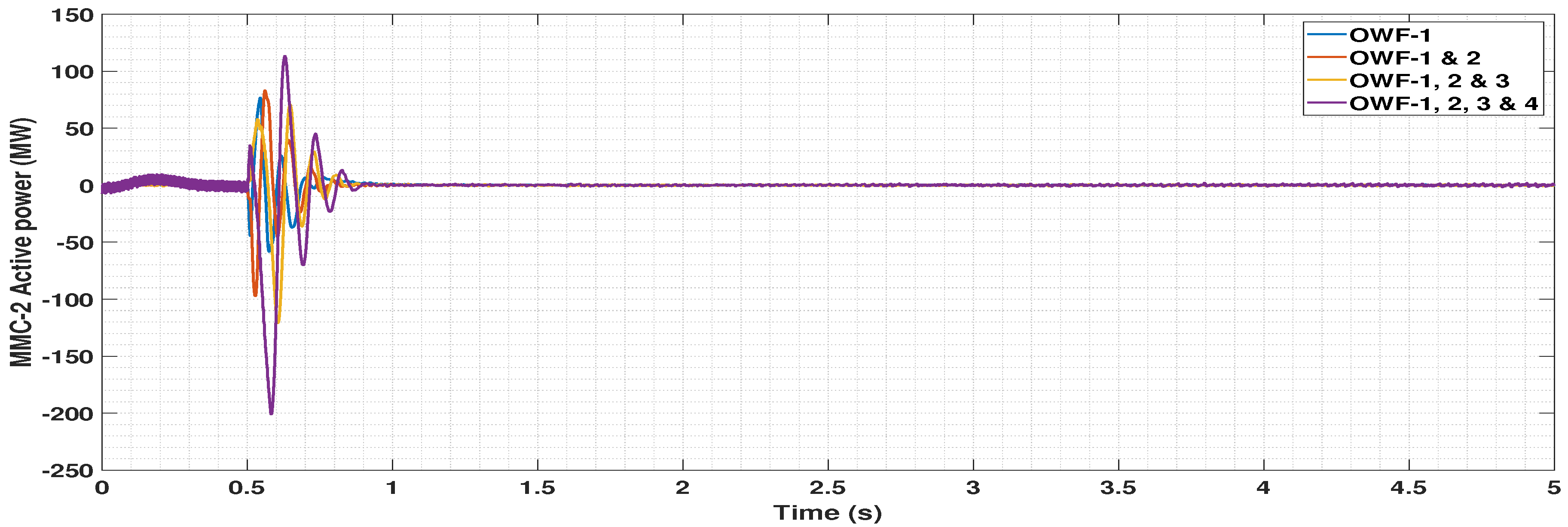
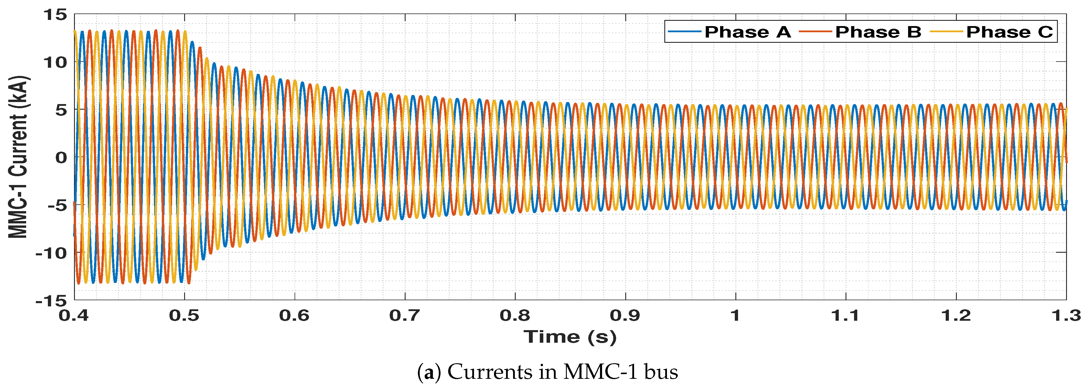
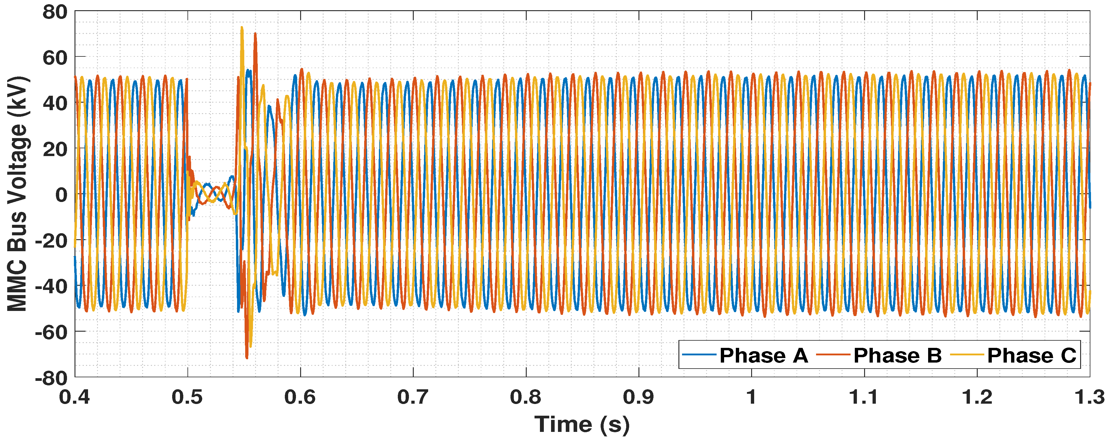
5.4.1. Disconnection of One OWF
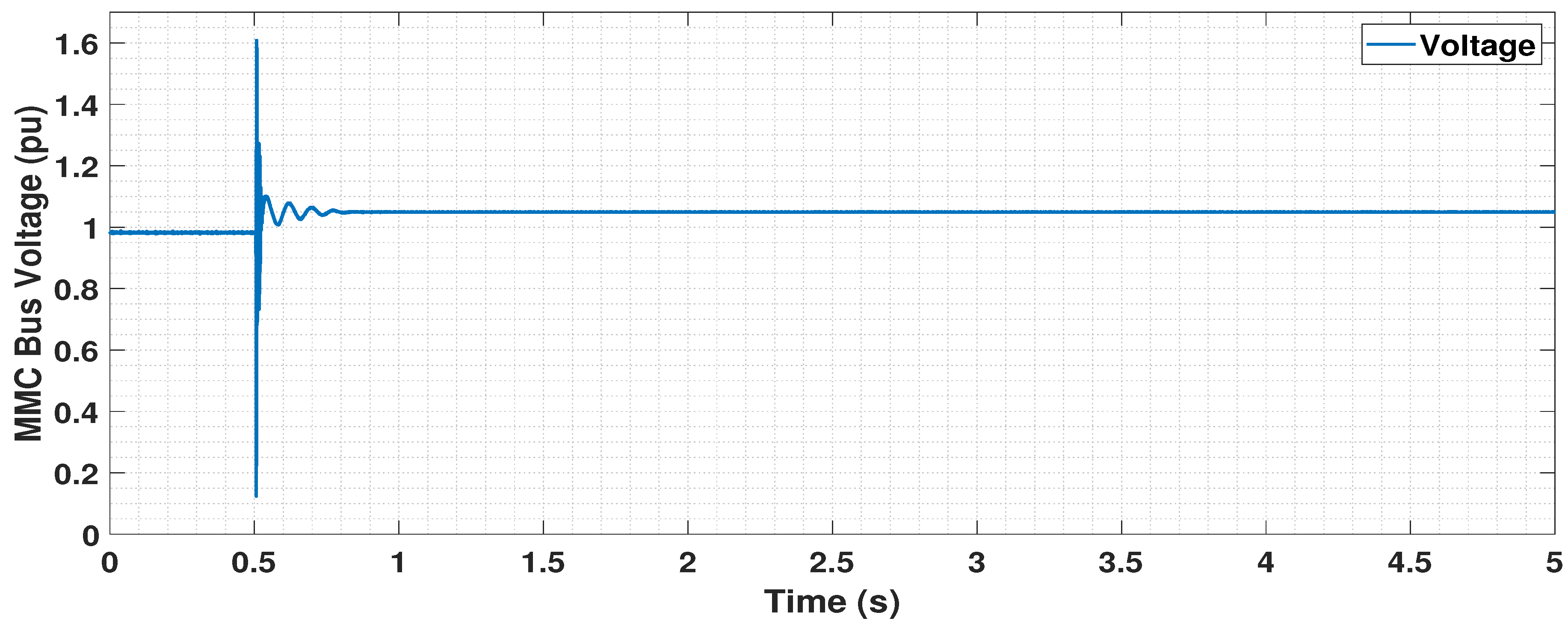
5.4.2. Circuit Breaker Operation Logic
6. Conclusions
Author Contributions
Funding
Data Availability Statement
Acknowledgments
Conflicts of Interest
References
- UNFCCC. Adoption of the Paris agreement. COP. In 25th Session Paris; UNFCCC: Rio de Janeiro, Brazil; New York, NY, USA, 2015; Volume 30, Available online: https://unfccc.int/sites/default/files/english_paris_agreement.pdf (accessed on 29 January 2021).
- Vision—North Sea Wind Power Hub. 2020. Available online: https://northseawindpowerhub.eu/vision/ (accessed on 26 January 2021).
- TenneT Develops First 2 GW Offshore Grid Connection with Suppliers. Daily Offshore Wind News, 13 February 2020.
- The First Hub-and-Spoke Energy Island—North Sea Wind Power Hub. 2020. Available online: https://northseawindpowerhub.eu/the-first-hub-and-spoke-energy-island/ (accessed on 26 January 2021).
- Bolik, S.; Ebner, G.; Elahi, H.; Gomis Bellmunt, O.; Hjerrild, J.; Horne, J.; Kilter, J.; Rimez, J.; Temtem, S.; Visiers Guixot, M. HVDC Connection of Offshore Wind Power Plants; Technical Brochure 619; CIGRE Working Group B4.55. 2015. Available online: https://e-cigre.org/publication/619-hvdc-connection-of-offshore-wind-power-plants (accessed on 29 January 2021).
- Peralta, J.; Saad, H.; Dennetière, S.; Mahseredjian, J.; Nguefeu, S. Detailed and Averaged Models for a 401-level MMC-HVDC system. IEEE Trans. Power Deliv. 2012, 27, 1501–1508. [Google Scholar] [CrossRef]
- Telaretti, E.; Graditi, G.; Ippolito, M.; Zizzo, G. Economic feasibility of stationary electrochemical storages for electric bill management applications: The Italian scenario. Energy Policy 2016, 94, 126–137. [Google Scholar] [CrossRef]
- Mohseni, M.; Islam, S.M. Review of international grid codes for wind power integration: Diversity, technology and a case for global standard. Renew. Sustain. Energy Rev. 2012, 16, 3876–3890. [Google Scholar] [CrossRef]
- HVDC Technology for Offshore Wind is Maturing; ABB: Zürich, Switzerland, 2018; Available online: https://new.abb.com/news/detail/8270/hvdc-technology-for-offshore-wind-is-maturing (accessed on 26 January 2021).
- Korai, A.W. Dynamic Performance of Electrical Power Systems with High Penetration of Power Electronic Converters: Analysis and New Control Methods for Mitigation of Instability Threats and Restoration. Ph.D. Thesis, Universität Duisburg-Essen, Duisburg, Germany, 2019. [Google Scholar] [CrossRef]
- Lescale, V.; Holmberg, P.; Ottersten, R.; Hafner, Y. Parallelling offshore wind farms HVDC ties on offshore side. Proc. CIGRE 2012 2012. [Google Scholar]
- Ganesh, S.; Perilla, A.; Torres, J.; Palensky, P.; van der Meijden, M. Validation of EMT Digital Twin Models for Dynamic Voltage Performance Assessment of 66 kV Offshore Transmission Network. Appl. Sci. 2021, 11, 244. [Google Scholar] [CrossRef]
- RTDS Technologies Inc. Novacor. 2020. Available online: https://knowledge.rtds.com/hc/en-us/articles/360034290474-NovaCor- (accessed on 26 January 2021).
- Vrana, T.K.; Yang, Y.; Jovcic, D.; Dennetière, S.; Jardini, J.; Saad, H. The CIGRE B4 DC grid test system. Electra 2013, 270, 10–19. [Google Scholar]
- World’s Most Powerful Offshore Wind Turbine: Haliade-X 12 MW | GE Renewable Energy. 2020. Available online: https://www.ge.com/renewableenergy/wind-energy/offshore-wind/haliade-x-offshore-turbine (accessed on 26 January 2021).
- RTDS Technologies Inc. PB5 Card. 2020. Available online: https://knowledge.rtds.com/hc/en-us/articles/360034285894-PB5-Card (accessed on 26 January 2021).
- Ryndzionek, R.; Sienkiewicz, L. Evolution of the HVDC Link Connecting Offshore Wind Farms to Onshore Power Systems. Energies 2020, 13, 1914. [Google Scholar] [CrossRef] [Green Version]
- CIGRE Working Group B4.37. VSC Transmission. Technical Brochure 269. 2005. Available online: https://e-cigre.org/publication/269-vsc-transmission (accessed on 26 January 2021).
- RTDS Technologies Inc. MMC Modeling. 2020. Available online: https://knowledge.rtds.com/hc/en-us/articles/360039628773-MMC-Modeling (accessed on 26 January 2021).
- Sharifabadi, K.; Harnefors, L.; Nee, H.P.; Norrga, S.; Teodorescu, R. Design, Control, and Application of Modular Multilevel Converters for HVDC Transmission Systems; John Wiley & Sons: Hoboken, NJ, USA, 2016. [Google Scholar]
- Erlich, I.; Korai, A.; Neumann, T.; Koochack Zadeh, M.; Vogt, S.; Buchhagen, C.; Rauscher, C.; Menze, A.; Jung, J. New Control of Wind Turbines Ensuring Stable and Secure Operation Following Islanding of Wind Farms. IEEE Trans. Energy Convers. 2017, 32, 1263–1271. [Google Scholar] [CrossRef]
- CIGRE Working Group B4.57. Guide for the Development of Models for HVDC Converters in a HVDC Grid. Tech. Rep.. 2014. Available online: https://e-cigre.org/publication/604-guide-for-the-development-of-models-for-hvdc-converters-in-a-hvdc-grid (accessed on 26 January 2021).
- Saad, H.A. ModÉlisation et Simulation D’Une Liaison Hvdc de Type Vsc-Mmc. Ph.D. Thesis, Polytechnique Montréal, Montreal, QC, Canada, 2015. [Google Scholar]
- RTDS Technologies Inc. RSCAD Modules. 2020. Available online: https://knowledge.rtds.com/hc/en-us/articles/360037537653-RSCAD-Modules (accessed on 26 January 2021).


| Small Time Step Block | Core Assignment |
|---|---|
| OWF-1 | 4 |
| OWF-2 | 1 |
| OWF-3 | 3 |
| OWF-4 | 1 |
| Small Time Step Block | Core Assignment |
|---|---|
| MMC-1 | 3 |
| MMC-2 | 2 |
Publisher’s Note: MDPI stays neutral with regard to jurisdictional claims in published maps and institutional affiliations. |
© 2021 by the authors. Licensee MDPI, Basel, Switzerland. This article is an open access article distributed under the terms and conditions of the Creative Commons Attribution (CC BY) license (http://creativecommons.org/licenses/by/4.0/).
Share and Cite
Ganesh, S.; Perilla, A.; Rueda Torres, J.; Palensky, P.; Lekić, A.; van der Meijden, M. Generic EMT Model for Real-Time Simulation of Large Disturbances in 2 GW Offshore HVAC-HVDC Renewable Energy Hubs. Energies 2021, 14, 757. https://doi.org/10.3390/en14030757
Ganesh S, Perilla A, Rueda Torres J, Palensky P, Lekić A, van der Meijden M. Generic EMT Model for Real-Time Simulation of Large Disturbances in 2 GW Offshore HVAC-HVDC Renewable Energy Hubs. Energies. 2021; 14(3):757. https://doi.org/10.3390/en14030757
Chicago/Turabian StyleGanesh, Saran, Arcadio Perilla, Jose Rueda Torres, Peter Palensky, Aleksandra Lekić, and Mart van der Meijden. 2021. "Generic EMT Model for Real-Time Simulation of Large Disturbances in 2 GW Offshore HVAC-HVDC Renewable Energy Hubs" Energies 14, no. 3: 757. https://doi.org/10.3390/en14030757
APA StyleGanesh, S., Perilla, A., Rueda Torres, J., Palensky, P., Lekić, A., & van der Meijden, M. (2021). Generic EMT Model for Real-Time Simulation of Large Disturbances in 2 GW Offshore HVAC-HVDC Renewable Energy Hubs. Energies, 14(3), 757. https://doi.org/10.3390/en14030757