Integration and Optimal Control of MicroCSP with Building HVAC Systems: Review and Future Directions

Abstract

Heating, ventilation, and air-conditioning (HVAC) systems are omnipresent in modern buildings and are responsible for a considerable share of consumed energy and the electricity bill in buildings. On the other hand, solar energy is abundant and could be used to support the building HVAC system through cogeneration of electricity and heat. Micro-scale concentrated solar power (MicroCSP) is a propitious solution for such applications that can be integrated into the building HVAC system to optimally provide both electricity and heat, on-demand via application of optimal control techniques. The use of thermal energy storage (TES) in MicroCSP adds dispatching capabilities to the MicroCSP energy production that will assist in optimal energy management in buildings. This work presents a review of the existing contributions on the combination of MicroCSP and HVAC systems in buildings and how it compares to other thermal-assisted HVAC applications. Different topologies and architectures for the integration of MicroCSP and building HVAC systems are proposed, and the components of standard MicroCSP systems with their control-oriented models are explained. Furthermore, this paper details the different control strategies to optimally manage the energy flow, both electrical and thermal, from the solar field to the building HVAC system to minimize energy consumption and/or operational cost.

1. Introduction

One of the major challenges that the world is facing today is climate change. The repercussions of climate change are expected to be devastating in the future compared to what several countries are experiencing currently. Indeed, heat waves, with very high and unprecedented temperatures, struck several countries breaking records and reaching up to 41 °C in South Korea in 2018 [1] and 48 °C in Portugal in 2003 [2]. On the other hand, the lowest temperature ever recorded on earth (−93.2 °C) was reported in Antarctica in 2010 [3]. These extreme weather conditions cause high energy consumption in buildings due to the increased demand for both cooling and heating in order to ensure the temperature comfort of the users. Furthermore, the International Energy Agency (IEA) reported that building direct emissions contributed to 28% of the global fossil fuel-based greenhouse gas (GHG) emissions in 2019 [4]. This leads to a vicious cycle and a snowball effect that, if not addressed quickly and appropriately, could have drastic consequences on our planet in the near future.

About 45% of the world’s primary energy resources are consumed by buildings [5]. Heating, ventilation, and air-conditioning (HVAC) systems are among the most energy-consuming loads in a building and are responsible for 40% of its energy consumption [5]. Thus, HVAC systems are good candidates for energy efficiency programs and will benefit greatly from integration with solar energy.

Solar energy is the principal and most abundant source of clean energy on the planet [6]. Indeed, the total annual energy consumption of the entire world can be met by solar collectors with 20% efficiency, covering a thousandth of the terrestrial sphere [7]. Solar energy is an environment-friendly alternative for fossil fuel-based electricity generation and heat production that is becoming more cost-competitive. Furthermore, the omnipresence of solar irradiation can be leveraged for distributed generation, hence avoiding the expensive alternative of grid extension. Solar energy can reduce the transmission energy losses and avoid fossil fuel-fired electricity generation, particularly in remote areas in Africa [8] which has a very low electricity coverage rate while possessing a large potential of solar irradiation [9].

This paper builds upon our prior works [10,11,12,13,14,15,16,17,18,19,20,21,22] in the area of modeling and control of solar-assisted HVAC systems in buildings, particularly the integration of micro-scale concentrated solar power (MicroCSP) into building HVAC systems. The main objective of this review paper is to give an overview of the MicroCSP technology and how it can be optimally controlled to get the full benefit from its integration into building HVAC systems. More specifically, this paper presents the different components of a typical MicroCSP system, and then it discusses various integration architectures of MicroCSP into building HVAC systems. Moreover, the required modeling of the MicroCSP components is detailed and the benefit of optimal model-based control of MicroCSP and building HVAC in tandem is explained. Finally, this work provides a unique benchmark of optimal control strategies for MicroCSP integrated into the building HVAC system since it aggregates comparable results from extensive studies performed on the same testbed using the same experimental measurements.

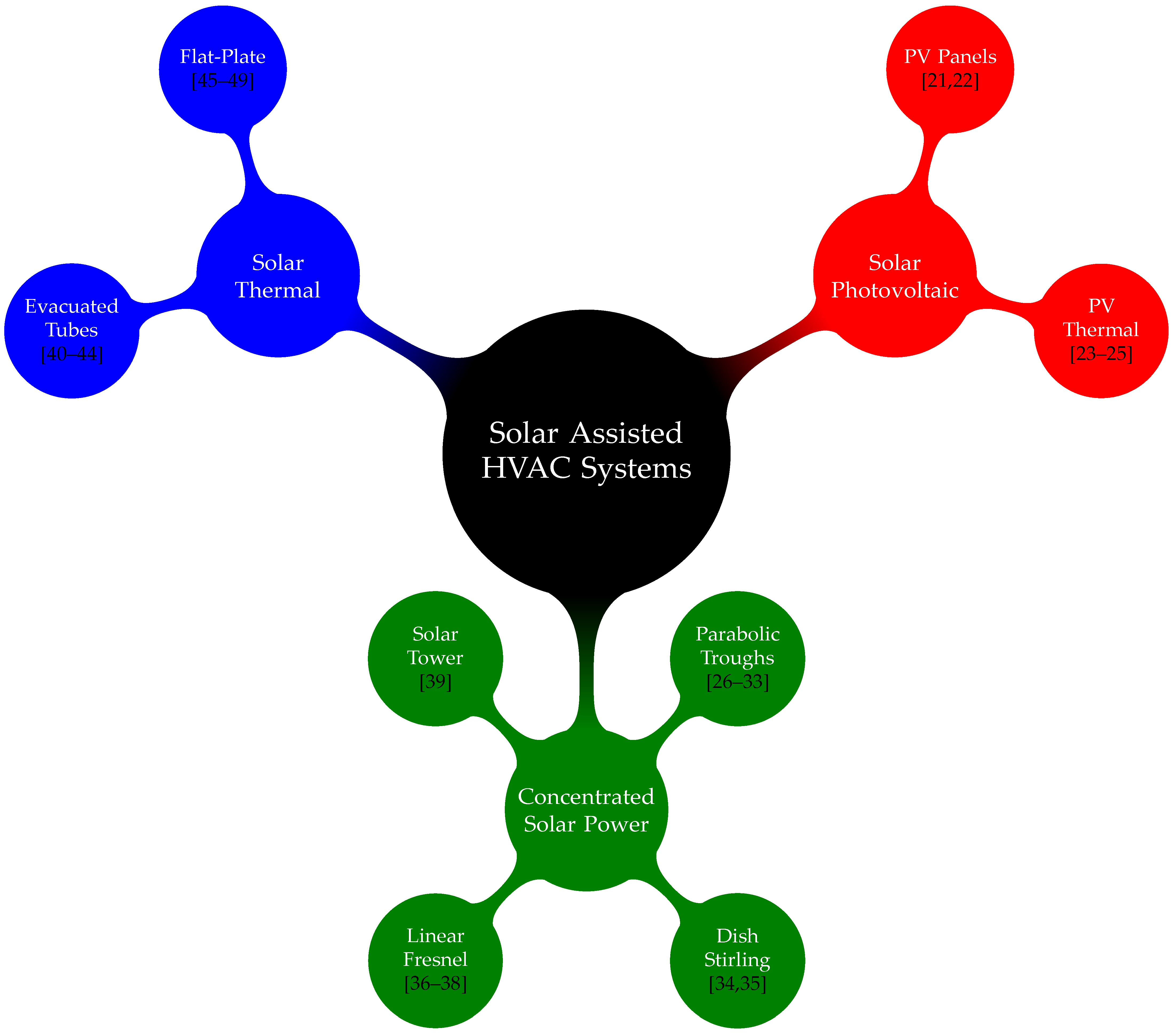
2. Solar-Assisted HVAC Systems

To understand the benefits of MicroCSP integration into HVAC systems, one should review the existing thermal-assisted HVAC systems, especially the solar-based systems. The three main technologies utilized to harvest solar power are: (i) the photovoltaic (PV) cell technology commonly employed to generate electrical power; (ii) the solar thermal power technology which is mainly used for heat generation; and (iii) the concentrated solar power (CSP) technology that generates both electrical and thermal energy. Figure 1 categorizes the solar-assisted HVAC systems into three main categories, based on the solar energy technology utilized in the system.

Table 1. Non-MicroCSP identified Thermal-assisted HVAC systems.

Thermal Assisted HVAC Plants	Country	COP */EER *	Primary Energy System	TES *	HTF *	Ref.
Cardiff Univ. STACS System	UK	0.7	Evacuated tubes	Cold Water Single-Tank	Water	[44]
CIESOL building	Spain	0.6	Flat-plate	Hot Water Two-Tank	Water	[48]
Eng. School of Seville Solar Plant	Spain	1.34	Linear Fresnel Reflectors	None	Water	[50]
Fraunhofer Institute (UMSICHT) Plant	Germany	0.37–0.8	Evacuated tubes	Hot Water Single-Tank	Water	[42]
Sannio Univ. Test Facility	Italy	3	MicroCHP	None	None	[51,52]
SERT Test Building	Thailand	0.5	Evacuated tubes	Hot Water Single-Tank	Water	[43]
Shanghai Jiao Tong Univ. Exptl. Setup	China	0.34–0.44	Compound Parabolic Collectors	Hot Water Single-Tank	Water	[53]
SOLERA Project	Germany	0.6	Linear Fresnel Reflectors	None	None	[54]
Team UOW Solar Decathlon House	China/Australia	2.1	Air-based photovoltaic thermal	Phase Change Materiel	Air	[55,56]
Univ. Carlos III de Madrid Solar Facility	Spain	0.33	Flat-plate	Hot Water Single-Tank	Water	[47]
Univ. of New Mexico ME Building	USA	3.8	Flat-plate and Evacuated tubes	Hot Water Single-Tank	Water	[45,46]
Univ. of Saint Pierre Pilot Plant	France	1.5–2.5	Flat-plate	Hot Water Single-Tank	Water	[49]
Univ. of Tech. Sydney Exptl. System	Australia	3.2–5.4	Evacuated tubes	Hot Water Single-Tank	Water	[40,41]

* COP, EER, TES, and HTF stand for coefficient of performance, energy efficiency ratio, thermal energy storage, and heat transfer fluid, respectively.

lists some examples of the solar-assisted HVAC systems reported in the literature. It can be noticed that water and air are the most used heat transfer fluid (HTF) in thermal-assisted HVAC systems since they can absorb the heat in the primary energy system while keeping the temperatures in the allowed operating range for the HVAC systems.

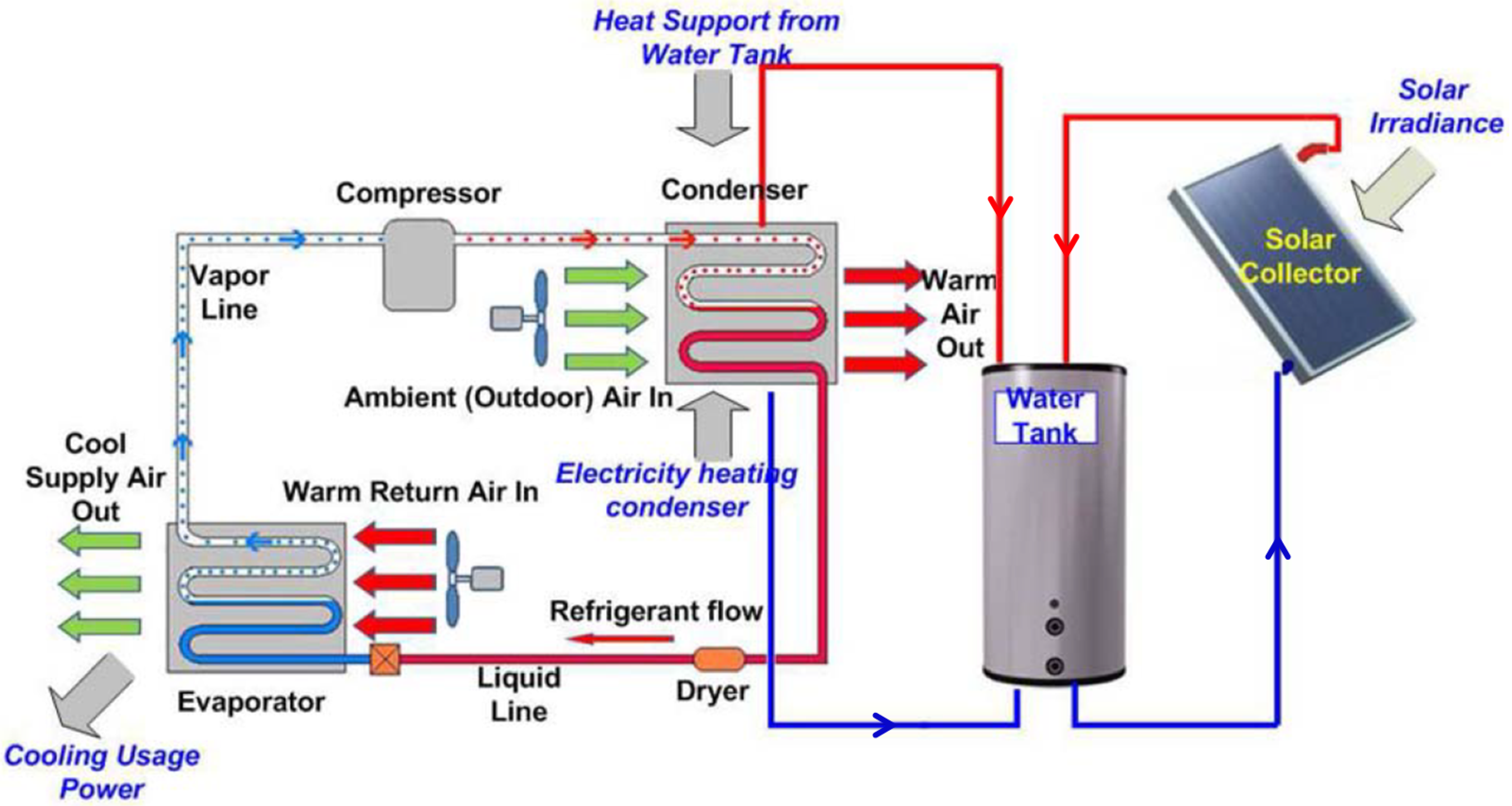
2.1. Solar Thermal-Assisted HVAC Systems for Buildings

The combination of a solar-thermal system with HVAC systems in buildings to lower energy consumption and cost is quite common in the literature. One of the main technologies used are evacuated tubes and flat plates used by the authors of [45,46] for a solar-thermal-assisted HVAC system in a university campus building that generates thermal energy. This thermal energy is first stored in a hot water tank and then dispatched either to the heating coil or the absorption chiller that supplies the cold water tank. Look-ahead scheduling based on day-ahead temperature and solar irradiation predictions allowed the authors to save 30% of the annual energy cost. Cioccolanti et al. [57] investigated the utilization of a small-scale trigeneration system using evacuated flat-plate collectors to generate electricity, cooling, and heating for a building. They demonstrated that the optimal sizing of the storage system can increase the overall efficiency by 6.5%. Nguyen et al. [58] presented hybrid solar-assisted HVAC and water heating, as shown in Figure 2, where a rolling stochastic optimization technique was used for the smart scheduling of energy to significantly reduce the energy cost of the building by 50% compared to the conventional HVAC and water heating system.

2.2. Solar Photovoltaic (PV)-Assisted HVAC Systems

Solar energy can be harnessed by the well-known photovoltaic (PV) systems that use photovoltaic cells to convert solar radiation into electrical energy. PV-thermal, on the other hand, is a hybrid solar-based system that can cogenerate both electricity and low-grade heat. Compared to the conventional PV technology, PV-thermal has higher overall efficiency since its heat extraction mechanism has a two-fold advantage: (i) it cools off the photovoltaic cells which increases the efficiency and life cycle of the PV cells; and (ii) the extracted low-grade heat can be exploited by HVAC systems and/or used for providing hot water.

Ramos et al. [23] coupled PV-thermal panels with absorption chillers and heat pumps (HP) in different topologies. For each topology, the authors ran simulations for ten different sites in Europe showing that the proposed integrated system can fulfill the entire cooling load and up to 60% of the heating load. Gu et al. [25] performed an economic analysis of a building integrating PV-thermal panels in Sweden for electrical and thermal energy cogeneration. By carrying out a sensitivity analysis on eleven factors based on the Monte Carlo method, they concluded that PV-thermal panels are more lucrative for areas that have higher solar irradiance and higher heating rates. In [24], the authors investigated the trigeneration of heating, cooling, and electricity by a PV-thermal solar field in tandem with absorption chillers. Based on experimental data collected from a university campus testbed, they conducted an economic evaluation that compares the proposed system with two other solar-thermal assisted systems, one composed of evacuated tube collectors and the other consisting of PV panels. They demonstrated that the payback time of the proposed trigeneration system is 2.3 times faster than the system based on evacuated tube collectors and 2.7 times faster than the PV-based system, while significantly reducing the GHG emissions.

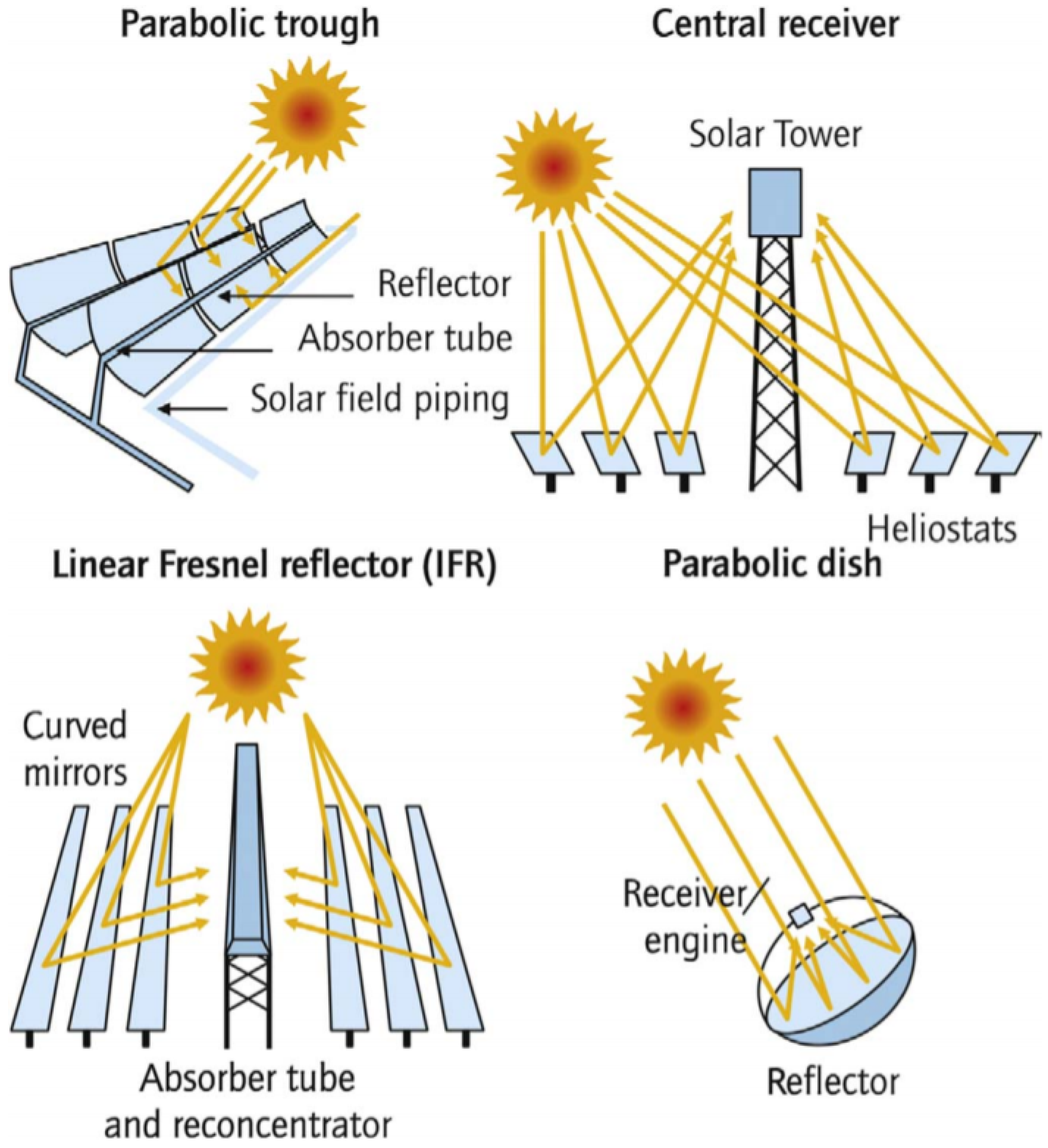
2.3. Concentrated Solar Power (CSP)-Assisted HVAC Systems

The CSP technology has been widely used in large-scale power generation plants since the 1973 energy crises [60] by converting high-temperature heat into electrical energy through efficient conventional turbines. Nevertheless, CSP was originally utilized for small-scale thermal-mechanical water pumping systems up to 100 kW [61] before being adopted for large power plants. As shown in Figure 1, the CSP systems can be classified into four main types, depending on the collectors technology: the solar tower collectors, the parabolic trough collectors, the linear Fresnel collectors, and the dish Stirling.

Micro-scale cogenerated heat and power (MicroCHP) is a conventional decentralized cogeneration system widely used for the production of electricity and domestic heating [51,52,62,63]. Their co-cogeneration capabilities and full dispatchability make MicroCHP systems promising for integration into building HVAC systems. However, their primary source of energy is either biomass-fired boilers or fossil fuel-fired internal combustion engines, which contribute to GHG emissions. The trend of green distributed generation made researchers consider a solar-based alternative by downsizing the CSP technology into micro-scale concentrated solar power (MicroCSP) systems with a rated power up to 1 MW [64]. MicroCSP has the same cogeneration capabilities as MicroCHP; however, it uses solar as a primary source of energy instead of fuel and biomass.

In terms of thermodynamics, the MicroCSP power cycle is comparable to the conventional CSP plant. Indeed, similar to MicroCHP systems, the power engines used in MicroCSP systems are, in most cases, based on the ORC that imitates the conventional Ranking cycle, but, instead of using water as a working fluid, it utilizes an organic fluid to convert low-grade thermal energy into electrical energy [65]. Even though the thermal efficiency of the ORC engine is intrinsically low, the building can harvest the low-grade waste heat of the ORC engine to fulfill the required thermal energy, hence improving the overall efficiency [66]. Moreover, the combination of ORC engines with solar collectors is a good candidate for renewable energy integration into buildings as they are becoming more competitive with PV panels in terms of energy pricing [67].

MicroCSP systems can provide both electrical power and heating source that can be utilized in building HVAC systems. Our previous work [20] shows that, by integrating MicroCSP into the HVAC system, buildings can save 8% more energy than what they could have saved by using PV.

In 2011, the Department of Energy (DOE) of the United States started the SunShot Initiative with the objective of increasing the competitiveness of solar power by decreasing the investment in utility-scale solar-based power plants by 75% making it around $1000/kW [68]. The initiative has also set a goal for 2030 to reduce the levelized cost of electricity (LCOE) of solar energy in residential applications by 90%. Due to the potential of CSP technology in residential applications, the LCOE for CSP technology energy is expected to be less than $0.05/kWh in 2030 compared to $0.21/kWh in 2010 [68]. Furthermore, the DOE allocated, in 2018, a $72 million budget envelope to develop the CSP systems of the future [69].

Table 2. Identified MicroCSP systems.

Country	Solar Field	HTF	Net Power	TES	Ref.
Australia	PTC	Thermal oil	300 kW	None	[26]
Australia	PTC	Pressurized water	175 kW	None	[26]
Belgium	PTC	Thermal oil	2.8 kW	Single-tank thermocline (pebble-bed)	[27]
China	Solar Tower	Water/Steam	1 MW	Two stages: saturated steam/oil	[39]
Egypt	PTC	Steam	75 kW	None	[28]
India	Parabolic Dish	Helium	9 kW	None	[34]
India	PTC	Therminol VP-1	1 MW	None	[29]
Italy	LFR	Diathermic oil	1 MW	None	[36]
Italy	PTC	Molten salt	350 kW	2-tank direct (Molten salt)	[30]
Italy	Parabolic Dish	Water and propylenic glycol	11.5 kW	Single-tank direct (Hot water)	[35]
Lesotho	PTC	Monoethylene glycol	1 kW	None	[31]
Lesotho	PTC	Monoethylene glycol	3 kW	Single-tank thermocline (Packed-bed)	[32]
Morocco	LFR	Delco term solar E15	1 MW	Single-tank thermocline (Packed-bed)	[37]
Switzerland	LFR	HCFC123 and HFC134a	10–25 kW	None	[38]
USA	PTC	Propylene Glycol	3 kW	Single-tank thermocline (Packed-bed)	[33]

lists some of the MicroCSP systems that have been deployed either for research and demonstration purposes or for commercial usage. One can notice that solar fields for MicroCSP systems are mostly based on parabolic trough collectors (PTC). This is due to the fact that PTC is a mature technology that has been in use for years [61]. Besides, PTC-based solar fields are very easy to scale by simply connecting new arrays to the existing ones.

This paper explores the benefits and potentials of optimal integration of MicroCSP technology into the building HVAC system, in different topologies, and with different electricity price schemes. It also provides insights into the factors that differentiate MicroCSP from other thermal-assisted HVAC applications. Furthermore, it emphasizes the importance of optimal control of the MicroCSP and building HVAC system. Indeed, our previous study [20] concluded that designing optimal control frameworks that account for the dynamics of the MicroCSP and the building HVAC system can significantly reduce the energy consumption up to 70% compared to a conventional rule-based control scheme.

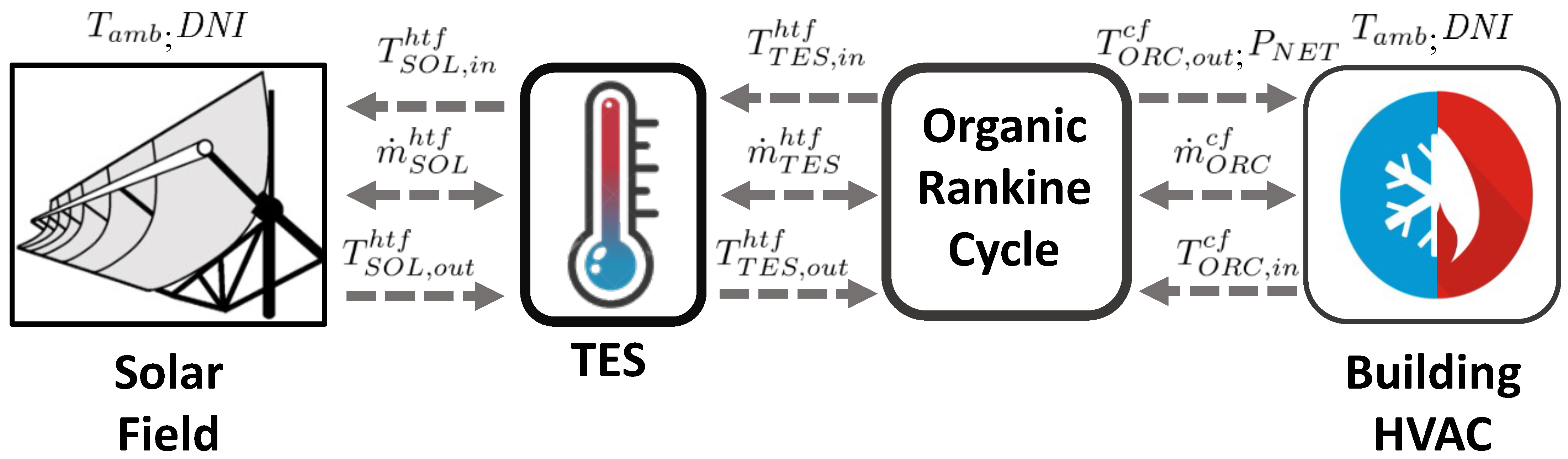
3. MicroCSP and Building HVAC Architectures

3.1. MicroCSP Components

The three main components of a MicroCSP system are: (1) a solar field with a concentrated solar power technology; (2) a thermal energy storage (TES) system; and (3) a power engine. Figure 3 presents the schematic of a sample MicroCSP system with a PTC-based solar field, a two-tank TES system, and an ORC engine. These components are explained in the following.

3.1.1. Solar Field

Different technologies can be used in a solar field to harvest solar energy; however, in MicroCSP systems, the solar field is composed of solar concentrator technologies, namely PTC, parabolic dish concentrators, linear Fresnel reflectors, and solar towers. Figure 4 presents the main types of solar concentrators in solar fields. All four types of solar concentrators utilize mirror reflectors to concentrate the sunbeam into either a linear tube that carries the HTF in the case of parabolic trough collectors (PTC) and linear Fresnel reflectors (LFR) or a focal point that holds the HTF in the case of solar towers and parabolic dish concentrators, as shown in

Table 3. Solar Concentrators Characteristics [64].

Concentrator Area	Focal Area	Tracking System	Concentration Ratio
Parabolic trough	Linear	Biaxial tracking	15–45
Parabolic dish	Punctual	Biaxial tracking	Up to 1000
Linear Fresnel reflector	Linear	Monoaxial tracking	10–40
Central receiver	Ponctual/Planar	Biaxial tracking (Heliostat)	1000–10,000

.

Solar towers can generate high-temperature HTF with a temperature ranging from 300 to 2000 °C [70] and are usually combined with conventional Rankine cycle engines to produce electricity efficiently. Depending on the solar field area, both parabolic troughs and linear Fresnel reflectors can be coupled to the conventional Rankine cycle with high-temperature HTF or to ORC engines with low-temperature HTF. The parabolic dish concentrators technology, on the other hand, is often in tandem with Stirling engines exploiting low-temperature HTF to produce electricity. The solar concentrators efficiency depends essentially on the mirrors reflectivity and the receiver absorptance.

3.1.2. Thermal Energy Storage (TES)

TES systems have great benefits in solar electricity generation systems as they can: (i) shift energy production to meet peak demand; (ii) counteract the inherent diurnal fluctuation of solar radiation; and (iii) extend the power production to nighttime.

Compared to other storage technologies such as batteries or flywheels, TES systems offer advantages when coupled with solar thermal applications. The main advantage is related to the form of the energy stored in the TES. This is because storing heat directly, before conversion in the power engine, avoids conversion losses related to the use of other forms of energy. Furthermore, storing heat in the TES systems reduces system complexity, which results in an extended life cycle and relatively low capital expenses for the MicroCSP system.

The thermal energy can be stored as thermo-chemical heat in reversible endothermic chemical reactions [72], latent heat in phase change materials (PCM) [73], or sensible heat [74]. Sensible heat systems can store energy for days, even months if well insulated, and have an efficiency that ranges from 50% to 90% [75]. PCM storage periods range from a few hours to several months, depending on the material chosen, and have an efficiency between 75% and 90% [75]. Chemical reaction-based storage systems have shorter storage periods from hours to days; however, their efficiency starts from 75% and can reach 100% in some cases [75]. For low-temperature CSP applications such as MicroCSP, sensible heat is the most effective option as PCM requires high temperatures and special piping to deal with pressure variations. Furthermore, MicroCSP systems do not require seasonal/annual thermal storage; instead, it relies on diurnal TES systems to store the thermal energy for short periods, allowing load shifting for optimal operations [76].

3.1.3. Thermal Power Engines

The solar thermal energy collected by the solar concentrators in the solar field is either stored in the TES or directly sent to the thermal power engine to be converted into electrical energy and low-grade heat. Thermal power engines are governed by thermodynamic cycles. One of the well-known and most used thermodynamics cycles in heat to electricity conversion is the conventional Rankine cycle using water as working fluid in most use cases [77]. Since the wet steam can be harmful to the turbine blades, power engines based on conventional Rankine cycle are not suitable for MicroCSP systems as they require high-temperature inputs [78].

An alternative to conventional Rankine cycles is the ORC, which is widely used in solar applications due to its capacity to exploit low-temperature heat and convert it into electrical energy by using an organic fluid with lower vaporization temperature instead of water. However, the reported efficiencies of ORC engines are very low and do not exceed 15% [79]. However, buildings can yet benefit from the cogenerated low-grade heat of the ORC engine to reduce their energy consumption and operational cost of the HVAC systems [20].

On the other hand, Stirling engines are known to have better efficiencies than ORC engines [80] and can accommodate different heat sources including solar dishes with efficiencies up to 64% [81]. The solar-powered Stirling engine is governed by the theoretical Stirling cycle, as shown in Figure 5. The solar to electrical efficiency can reach up to 32%, which the highest among CSP technologies [82]. On the other hand, the per kWh price of the solar-powered Stirling engine is more expensive than the other CSP technologies, which has prevented the wide adoption of this technology.

3.2. MicroCSP Integration to Building HVAC: Architectures and Energy Flows

The MicroCSP system collects the solar thermal energy at the solar field level. This collected energy is then stored in the TES before being dispatched into the thermal power engine to be converted into electrical and thermal energies that are used to assist the HVAC system to supply heating or cooling to the building. The architecture of the MicroCSP integration into the building HVAC system depends on the use case and heating/cooling demand of the building. In the following, four main categories for integrating MicroCSP and HVAC systems are explained.

3.2.1. Heating Cogeneration

The MicroCSP system is inherently capable of producing both electricity and heat. This capability can be leveraged for heating applications in buildings by integrating the MicroCSP system into the building HVAC system. Indeed, as we can see in Architecture (a) in Figure 6, the energy produced in the solar field is stored in the TES before being dispatched to the ORC engine following a specific control strategy. The ORC engine converts the high-temperature heat into electrical energy and cogenerated low-grade thermal energy. The electrical energy can supply heat pumps (HPs) of the HVAC system to provide heating to the building. As per the low-grade cogenerated energy, depending on the set points of the ORC engine, it is either injected directly to heat the building or utilized to preheat the supply air to the HPs.

3.2.2. Cooling Cogeneration

The combined MicroCSP and building HVAC system can also supply cooling to the building, as shown in Architecture (b) in Figure 6. In this application, the power produced by the ORC is supplied to the cooling system, while the low-grade heat is used by the absorption chiller [84] to provide cooling to the building.

This architecture tries to exploit the MicroCSP heat cogeneration to increase its overall efficiency. However, to avoid dependency of the cooling loads on the MicroCSP system and solar irradiation, an electricity-driven cooling system is also used and can be supplied by the electricity grid.

3.2.3. Combined Heat and Cooling Cogeneration

In some cases, buildings require both heating and cooling simultaneously. For instance, office buildings with on-premises computer servers and data centers would need cooling for the computing systems and heating for the office rooms in winter. In such a case, the MicroCSP system can be integrated into the building HVAC, as shown in Architecture (c) in Figure 6, so that the electricity produced by the ORC is supplied to the HVAC cooling system, while the heat is directly supplied to the building. However, the sizing of the MicroCSP and TES in this application is critical as the heating loads of the building will be entirely dependent on the MicroCSP production and consequently relying on solar irradiation.

3.2.4. Trigeneration

Architecture (d) is proposed as an alternative that improves Architecture (c) and provides both heating and cooling without being completely dependent on MicroCSP production. Indeed, as can be seen in Figure 6d, an electricity-driven heating system is added to the system so that the system can be supplied through the electricity grid in case the MicroCSP is not generating sufficient heat.

The four architectures presented in this section are the main system configurations that are employed to leverage the integration of a MicroCSP system into the building HVAC system depending on its applications or needs (heating, cooling, or both). Each architecture is composed of several components that interact with each other and these components need to be controlled so that they can operate optimally. Hence, modeling these components is essential to understand their dynamics, predict the system response, and design appropriate model-based control strategies.

4. Modeling of MicroCSP Integrated into HVAC Systems

The optimal control and integration of a MicroCSP system into the HVAC system of a building require modeling of every component of the overall system. Indeed, as shown in Figure 7, the models of the different component should exchange information in such a way that the overall model can reflect the behavior of the actual system in the most reliable manner. Such complex systems that combine thermal, thermo-mechanical, and electrical systems are challenging to model, particularly if one tries to develop high-fidelity models. This review focuses on the optimal control of the MicroCSP integrated into the building HVAC systems and does not focus on the issues of controlling the individual components. Thus, internal models of each MicroCSP components are not discussed, and only low-order control-oriented models that describe the energy flow and conversion through the systems are discussed. In this section, required governing equations to simulate MicroCSP for integration into HVAC systems are explained. The selected components are based on a common MicroCSP architecture. The models of the selected MicroCSP and HVAC components are experimentally validated in our previous works [10,12,13,15,85,86].

4.1. Solar Collectors

The solar field in MicroCSP applications is composed of short PTC (Figure 8) with less than 100 m of length, hence a one-dimensional collectors model is used [87]. For each time step t, starting with an inlet temperature $T_{htf}(t,0)$, HTF heat capacity $C_{htf}(t,0)$ and mass flow rate $\dot{m}$ are determined:

• Finding the solar power absorbed by 1-m section of the absorber:

  $$\begin{array}{ccc}\hfill {\dot{Q}}_{gain}& =& DNI·A_{aper}·{\tau }_{gl}·{\alpha }_{abs}·{\rho }_{cl}·{\eta }_{eff}·K\hfill \end{array}$$

  (1)

  where $DNI$ is the direct normal irradiation (W/m${}^2$); $A_{aper}$ is the aperture area and is determined by $A_{aper}=a·L$ (m${}^2$) with $L=1$ m; ${\tau }_{gl}$ is the transmittance of the glass envelope; ${\alpha }_{abs}$ is the absorptance of the absorber; ${\rho }_{cl}$ is reflectance of the clean mirror; ${\eta }_{eff}$ is the effective optical efficiency; and K is the incident angle modifier ($K=1$ for normal incidence).
• Finding the heat loss in 1-m section using the following correlation:

  $${\dot{Q}}_{loss}=a_0+a_1·(T_{htf}-T_{amb})+a_2·T_{htf}^2+a_3·T_{htf}^3+a_4·DNI·K·T_{htf}^2+\sqrt{V_w}·\left(a_5+a_6·(T_{htf}-T_{amb})\right)$$

  (2)

  where $V_w$ is the wind speed ($m/s$) and $a_k$ are the correlation coefficients given in reference [88].
• Calculating the power absorbed by the fluid over 1-m section:

  $$\begin{array}{ccc}\hfill {\dot{Q}}_{abs}& =& {\dot{Q}}_{gain}-{\dot{Q}}_{loss}\hfill \end{array}$$

  (3)
• Finding the outlet temperature of the 1-m section:

  $$\begin{array}{ccc}\hfill T_{SOL,out}^{htf}& =& T_{SOL,in}^{htf}+{\displaystyle \frac{{\dot{Q}}_{abs}}{{\dot{m}}_{htf}·C_{htf}}}\hfill \end{array}$$

  (4)

  where $C_{htf}$ and ${\dot{m}}_{htf}$ are, respectively, the heat capacity and the mass flow rate of the HTF.
• Finally, Steps 1–4 are repeated for each section to simulate the HTF temperature for the total length of the collectors.
  The inlet temperature of each 1-m section is the outlet temperature to the next collector section, while the inlet temperature of the first section is the outlet to the TES tank and the outlet temperature of the last section is the inlet temperature to the TES tank.

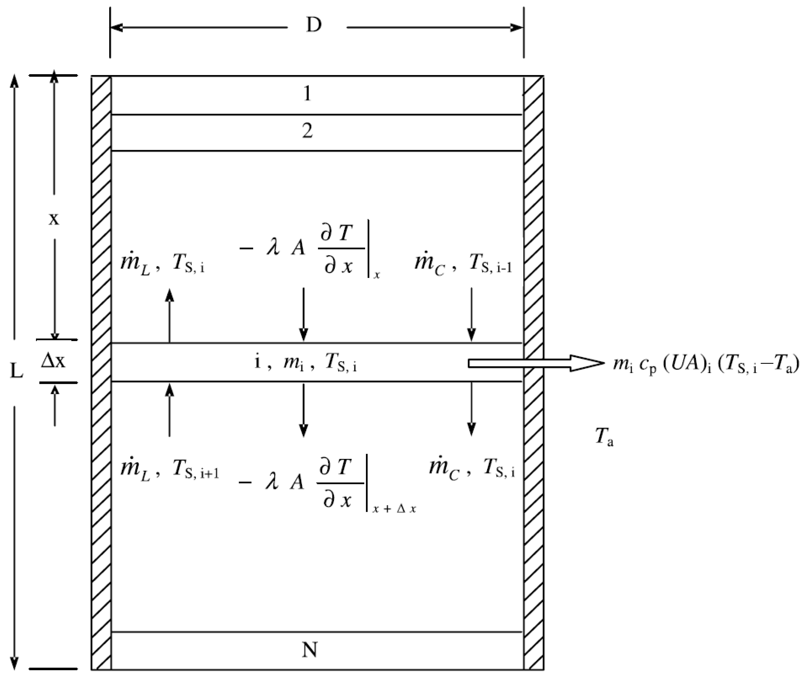
4.2. Thermal Energy Storage

Optimal control of MicroCSP operations involves controlling the energy flows within the TES system. The optimal controller must include the state of charge (SOC) of the TES in its constraints and maintain it within the allowed range. Since the TES systems in MicroCSP are not intended for long-term storage, the temperature of the HTF inside the TES tanks/reservoirs is assumed to remain constant over time. Hence, the SOC is estimated based on the mass/volume of the HTF, depending on the TES technology.

4.2.1. Single-Tank System

The simplest TES system used in MicroCSP applications is the single-tank system. The entire volume of the HTF is stored in the single reservoir where a thermocline forms a separating layer between the hot HTF at the top of the reservoir and the cold HTF at the bottom. The temperatures in both cold and hot HTF are assumed to remain constant over time; hence, the energy balance of the TES is given by [89]:

$$\begin{array}{c}\hfill E_{k+1}^{TES}=E_k^{TES}+\left({\eta }_{ch}·{\dot{Q}}_{SOL,k}-{\displaystyle \frac{{\dot{Q}}_{TES,k}}{{\eta }_{di}}}\right)·\Delta t\end{array}$$

(5)

where $E_k^{TES}$ is the energy in the TES at instant k; ${\eta }_{ch}$ and ${\eta }_{di}$ are charging and discharging efficiencies of the TES, respectively; ${\dot{Q}}_{SOL}$ is the thermal power from the PTC solar array; and ${\dot{Q}}_{TES}$ is the thermal power from the TES. Assuming that the TES reservoirs are well insulated, the charging and discharging efficiency of the TES can be set to 1 (i.e., ${\eta }_{ch}={\eta }_{di}=1$). Hence, the SOC of the TES is estimated at each time step k as follows

$$SO{C}_{k+1}^{TES}=SO{C}_k^{TES}+{\displaystyle \frac{{\sum }_k^{k+1}({\dot{Q}}_{SO{L}_k}-{\dot{Q}}_{{TES}_k})·\Delta t}{C_{TES}}}$$

(6)

where $C_{TES}$ is the heat capacity of the TES.

The presented single-tank model assumes that the HTF is separated by a thermocline into two volumes of HTF with constant temperature in each volume. However, a more detailed modeling approach can be used by considering the stratified thermocline single-tank TES system, as shown in Figure 9. It is a vertical cylinder divided horizontally into N equal layers called nodes. For each node, the energy balance equations are derived to capture the thermal energy coming from the solar field ($Q_{SOL}$), energy loss ($Q_{loss}$), and the dispatched energy to the ORC ($Q_{TES}$). A system of N differential equations is obtained [90].

4.2.2. Two-Tank System

The two-tank TES system is one of the well-known technologies used in MicroCSP applications. As the name suggests, the two-tank TES system is composed of two fully-mixed reservoirs that usually have a cylindrical shape and which can store the entire quantity of HTF. During charging mode, the low-temperature HTF leaves the “cold tank” into the solar fields to absorb the solar heat before accumulating at the “hot tank”. During discharging, the HTF is dispatched from the “hot tank” into the power engine. After transmitting its thermal energy to the working fluid (WF) of the ORC through the evaporator, the low-temperature HTF is pumped back to the “cold tank”. In terms of modeling, the equations applied to the single-tank TES system are valid for the two-tank TES system. Indeed, from a thermodynamic point of view, both systems are identical, since we have neglected the heat transfer between hot and cold fluid in the single-tank TES system. The only difference is that the boundaries between hot HTF and cold HTF are physical in the case of the two-tank TES system. Thus, the estimation of the SOC of two-tank TES at each time step k is the same as Equation (6); however, $C_{TES}$, in this case, is the TES heat capacity of both reservoirs.

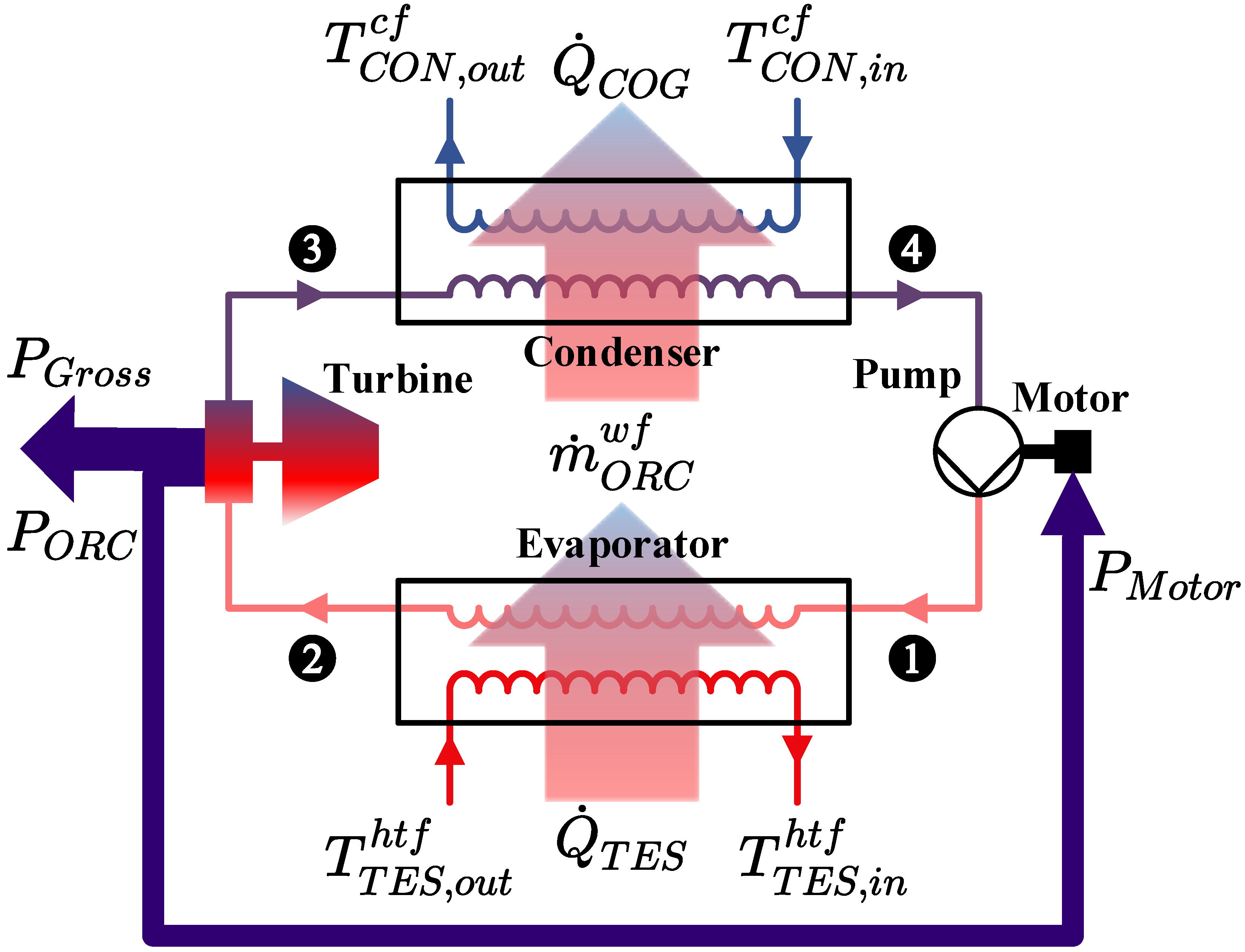
4.3. Thermal Power Engines

Dynamic modeling of Organic Ranking Cycles (ORC) engines for solar applications is well reported in the literature [88,91,92,93,94,95,96]. However, most of the dynamic ORC models are complex and computationally intensive, which makes them undesired for real-time optimal control applications. A control-oriented model of the ORC engine is detailed in this section.

Figure 10 presents the schematic of the ORC engine. The first process of the ORC cycle is evaporation. In this process, the heat absorbed by the evaporator is consisting of the heat supplied by the HTF dispatched from the TES to the WF through the heat exchanger, which is given by the following equation:

$$\begin{array}{ccc}\hfill {\dot{Q}}_{TES}& =& {\left(UA\right)}_{HE}·\Delta T_{LMTD}\hfill \end{array}$$

(7)

where U is the heat transfer coefficient of the plate heat exchanger derived from [97,98] and A is the plate area.

To determine the temperature differences and the heat transfer between the HTF and the WF at the heat exchanger, Mitterhofer and Orosz [33] proposed to use the logarithmic mean of the temperature differences (LMTD) between: (i) the HTF entering and the WF leaving the heat exchanger; and (ii) the HTF exiting the heat exchanger and the WF entering it.

$$\begin{array}{cc}\hfill \Delta T_{LMTD}& ={\displaystyle \frac{(T_{TES,out}^{htf}-T_2^{wf})-(T_{TES,in}^{htf}-T_1^{wf})}{ln{\displaystyle \frac{(T_{TES,out}^{htf}-T_2^{wf})}{(T_{TES,in}^{htf}-T_1^{wf})}}}}\end{array}$$

(8)

However, the LMTD method assumes that the temperatures of the HTF and the WF are constant and that the mass flow rate does not vary. This assumption is not valid for the control strategies that dispatch the HTF from the TES to have variable energy output from the power engine. Hence, the thermal power supplied to the ORC by the TES (${\dot{Q}}_{TES}$) can be estimated by [20]

$$\begin{array}{cc}\hfill {\dot{Q}}_{TES}& ={\dot{m}}_{TES}^{htf}·c_{p,htf}·(T_{TES,out}^{htf}-T_{TES,in}^{htf})\end{array}$$

(9)

The equations that govern the power flow in an ORC engine are

$$\begin{array}{cc}\hfill & P_{Gross}={\eta }_{gen}·{\dot{m}}_{ORC}^{wf}·(h_2-h_3)\hfill \end{array}$$

(10a)

$$\begin{array}{cc}\hfill & P_{Motor}={\displaystyle \frac{{\dot{m}}_{ORC}^{wf}·(h_1-h_4)}{{\eta }_{Motor}}}\hfill \end{array}$$

(10b)

$$\begin{array}{cc}\hfill & P_{ORC}=P_{Gross}-P_{Motor}\hfill \end{array}$$

(10c)

$$\begin{array}{cc}\hfill & {\dot{Q}}_{COG}={\dot{m}}_{ORC}^{wf}·(h_3-h_4)\hfill \end{array}$$

(10d)

$$\begin{array}{cc}\hfill & {\dot{Q}}_{TES}={\dot{m}}_{TES}^{htf}·c_{p,htf}·(T_{TES,out}^{htf}-T_{TES,in}^{htf})\hfill \end{array}$$

(10e)

where $P_{gross}$ and $P_{ORC}$ are, respectively, the gross and net electrical power generated by the turbine generator of the ORC; $P_{pump}$ is the power consumed by the ORC pump; ${\dot{Q}}_{COG}$ is the thermal power produced by the ORC; $h_1$, $h_2$, $h_3$, and $h_4$ are the enthalpies of the WF at the inputs and outputs of the turbine and the pump, respectively; ${\eta }_{pump}$ and ${\eta }_{gen}$ are the pump efficiency and turbine generator efficiency, respectively; ${\dot{m}}_{tes}$ and ${\dot{m}}_{wf}$ are the mass flow rates of the TES fluid and WF of the ORC, respectively; and $T_{ev,in}$ and $T_{ev,out}$ are, respectively, the temperatures at the input and output of the ORC evaporator. Further, it can be shown that:

$$\begin{array}{cc}\hfill & P_{ORC}=f\left({\dot{m}}_{TES}^{htf}\right)\hfill \end{array}$$

(11a)

$$\begin{array}{cc}\hfill & {\dot{Q}}_{COG}=g\left({\dot{m}}_{TES}^{htf}\right)\hfill \end{array}$$

(11b)

It should be noted that the control-oriented model of the ORC needs to be calibrated using experimental or manufacturer data.

4.4. HVAC System Modeling

There are different HVAC systems that can be used in buildings. Heat pumps (HP) are considered as one of the cleanest energy-efficient HVAC systems to supply heat to buildings. Here, an HP model is explained that is linked to a MicroCSP system below. The energy conversion in a HP is described by [10]:

$$\begin{array}{ccc}\hfill P_{i,t}^H& ={\displaystyle \frac{{\dot{m}}_{i,t}^{su}·c_{p,air}·({\mathcal{T}}_{i,t}^{su}-T_{i,t}^{HP})}{COP\left(T_t^{hot}\right)}}& \hfill \end{array}$$

(12)

where $P_{i,t}$ is the electrical power consumed by the HP; ${\dot{m}}_i^{su}$ is the the mass flow rate of supply air; ${\mathcal{T}}^{su}$ is the temperature of the supply air; $T_{i,t}^{HP}$ is the HP inlet air temperature; $T_t^{hot}$ is the heat source temperature of the HP; and $COP$ is the coefficient of performance of the HP which is a function of the heat source temperature.

The power consumed by the HVAC fan ($P_t^F$) is proportional to the cubic power of the mass flow rate of the HTF:

$$\begin{array}{ccc}\hfill P_t^F& ={\gamma }_F·{\left({\dot{m}}_{i,t}^{su}\right)}^3& \hfill \end{array}$$

(13)

where ${\gamma }_F$ is the fan coefficient.

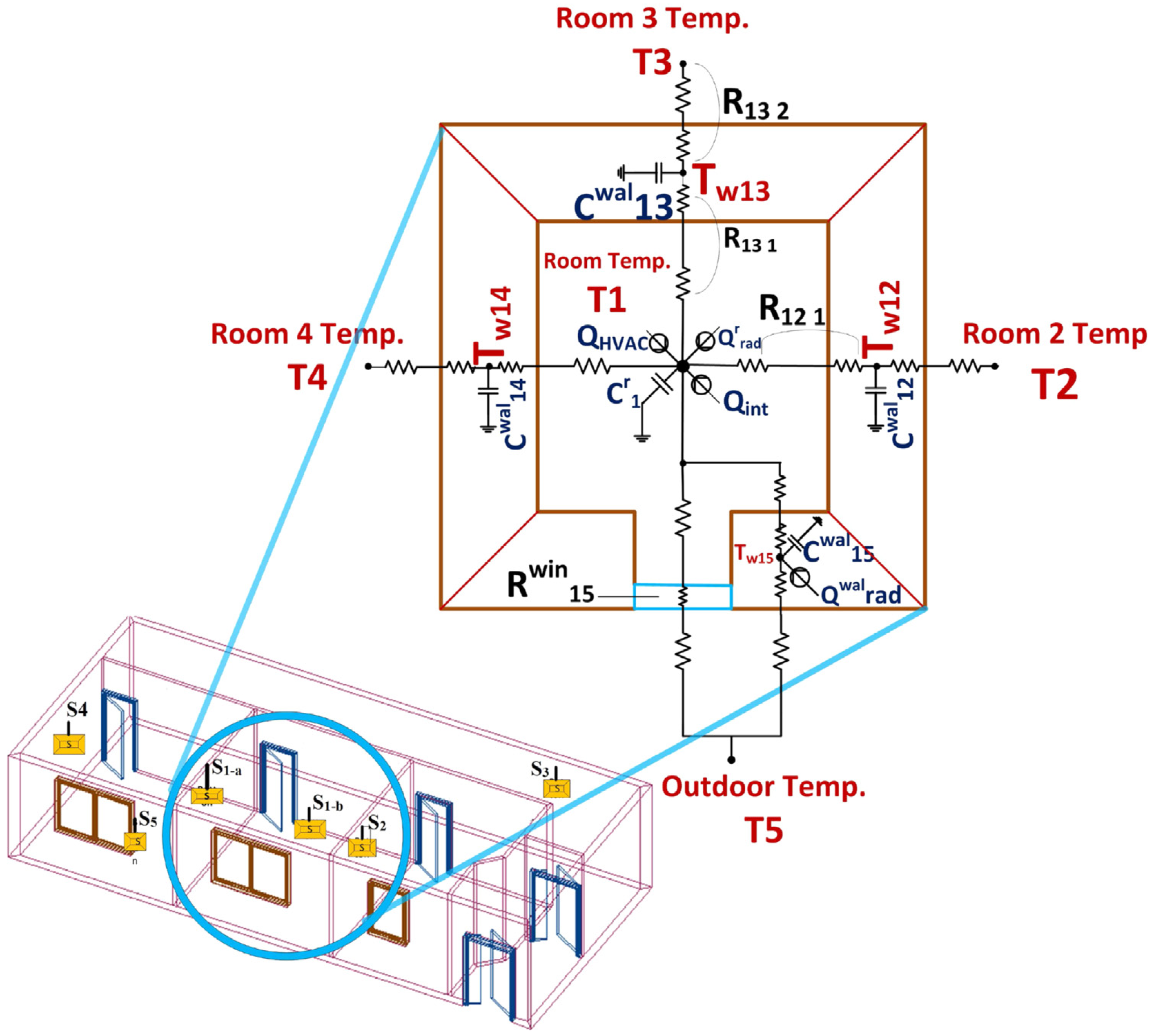
4.5. Building Thermal Model

The building thermal model is a central component in the design of the optimal HVAC control strategies since it simulates the thermal dynamics that affect the temperature of the rooms and HVAC load. The most common approach for having a control-oriented thermal model of the building is the nodal approach based on the thermal/electrical analogy where electrical elements such as current sources, resistors, and capacitors are utilized to, respectively, represent heat generation, heat transfer among building thermal zones, and heat storage in the room air and walls [10,11,13].

Using the thermal/electrical analogy, the building can be simulated as an electrical circuit where the nodes represent the rooms and walls of the building, connected through electrical elements. Figure 11 illustrates a sample room and its analogous electrical circuit. $i=1,\cdots ,q$ are the identifier numbers assigned to each room. The heat transfer of the walls between nodes i and j is given by [13]:

$$\begin{array}{ccc}\hfill C_{i,j}^w·\frac{d{T}_{i,j}^w}{dt}& =& \sum _{k\in {\mathcal{N}}_{i,j}^w}\frac{T_k^r-T_{i,j}^w}{R_k^{w_{i,j}}}+r_{i,j}^w·{\gamma }_{i,j}·A_{i,j}^w·Q_{i,j}^{rad}\hfill \end{array}$$

(14)

where $T_{i,j}^w$ is the wall temperature; $C_{i,j}^w$ is the wall heat capacity; $T_k^r$ is the temperature of the rooms neighboring to the wall; $R_k^{w_{i,j}}$ is the thermal resistance between the wall and the adjacent node k; $A_{i,j}^w$ and ${\gamma }_{i,j}$ are, respectively, the area and the radiation heat absorptivity of wall; $r^w$ identifies whether the wall is peripheral ($r^w$=1) or internal ($r^w$=0); $Q_{i,j}^{rad}$ is the radiative heat flux density on the wall; and ${\mathcal{N}}_{i,j}^w$ represents the set of the wall adjacent nodes.

The ith room temperature ($T_i^r$) is determined by the following equation [10]:

$$C_i^r·\frac{d{T}_i^r}{dt}=\sum _{k\in {\mathcal{N}}_i^r}\left[\frac{T_k-T_i^r}{R_{i,k}}+{\pi }_{i,k}·{\tau }_k^w·A_{i,k}^{win}·Q_i^{rad}\right]+{\dot{m}}_i^r·c_{p_{avg}}·(T_i^s-T_i^r)+{\dot{Q}}_i^{int}$$

(15)

where $C_i^r$ represents the heat capacity of the room air; $T_k$ is the temperature of adjacent node k; $T_i^s$, ${\dot{m}}_i^r$, and $c_{p_{avg}}$ are the temperature, the mass flow rate, and the average specific heat capacity of the supply air to the room, respectively; ${\pi }_{i,j}$ identifies whether there is a window between the room i and node k (${\pi }_{i,j}=1$) or not (${\pi }_{i,j}=0$); $A_{i,j}^{win}$ is the window’s area; ${\tau }_{i,j}^w$ is the transmissivity of window’s glass; $Q_i^{rad}$ is the radiative heat flux density on the window room i; and ${\dot{Q}}_i^{int}$ is the room’s intrinsic heat generation. ${\mathcal{N}}_i^r$ represents the set of the adjacent nodes to the room.

The disturbance to thermal model of the building is approximated as a linear function of $T_k^r\left(t\right)$, ${\dot{Q}}_i^{rad}\left(t\right)$ and ${\dot{Q}}_i^{int}\left(t\right)$ [11]:

$$\begin{array}{ccc}\hfill w\left(t\right)& =& a·T_k^r\left(t\right)+b·{\dot{Q}}_i^{rad}\left(t\right)+c·{\dot{Q}}_i^{int}\left(t\right)\hfill \end{array}$$

(16)

Using Equations (14)–(16), the state-space equation of the thermal model of the building is:

$$\begin{array}{cc}\hfill & \dot{x}\left(t\right)=f(x\left(t\right),u\left(t\right),w\left(t\right),t)\hfill \end{array}$$

(17a)

$$\begin{array}{cc}\hfill & y\left(t\right)=C·x\left(t\right)\hfill \end{array}$$

(17b)

where $x\left(t\right)\in {\mathbb{R}}^n$ is the state vector composed of the temperatures of the building’s rooms and walls; $y\left(t\right)\in {\mathbb{R}}^m$ is the output vector including the building rooms temperatures; and $u\left(t\right)$ is the input vector composed of the temperature and mass flow rate of the supply air. C is the output matrix with the proper dimensions to select room temperatures from the state vector.

5. Optimal Model Predictive Control

The dynamic models in Section 4 are implemented into optimal control frameworks to optimize combined MicroCSP and HVAC systems. In this section, the design of optimal model predictive controllers (MPCs) for the combined MicroCSP and building HVAC system is discussed. The designed MPCs are classified into three branches based on their control objectives, as shown in Figure 12. The first branch minimizes the building energy consumption. The second branch and the third branch minimize the electrical energy cost of the building considering the dynamic pricing and the electrical power grid status, respectively. Each branch in Figure 12 further lists the MPC frameworks designed and evaluated by our prior studies in [16,17,18,19,20,21,22]. This Section is organized into two parts. First, the structure and formulation of each of the designed MPC (Figure 12) is discussed. Next, the results of the MPCs in Figure 12 are discussed and compared with a common rule-based controller (RBC).

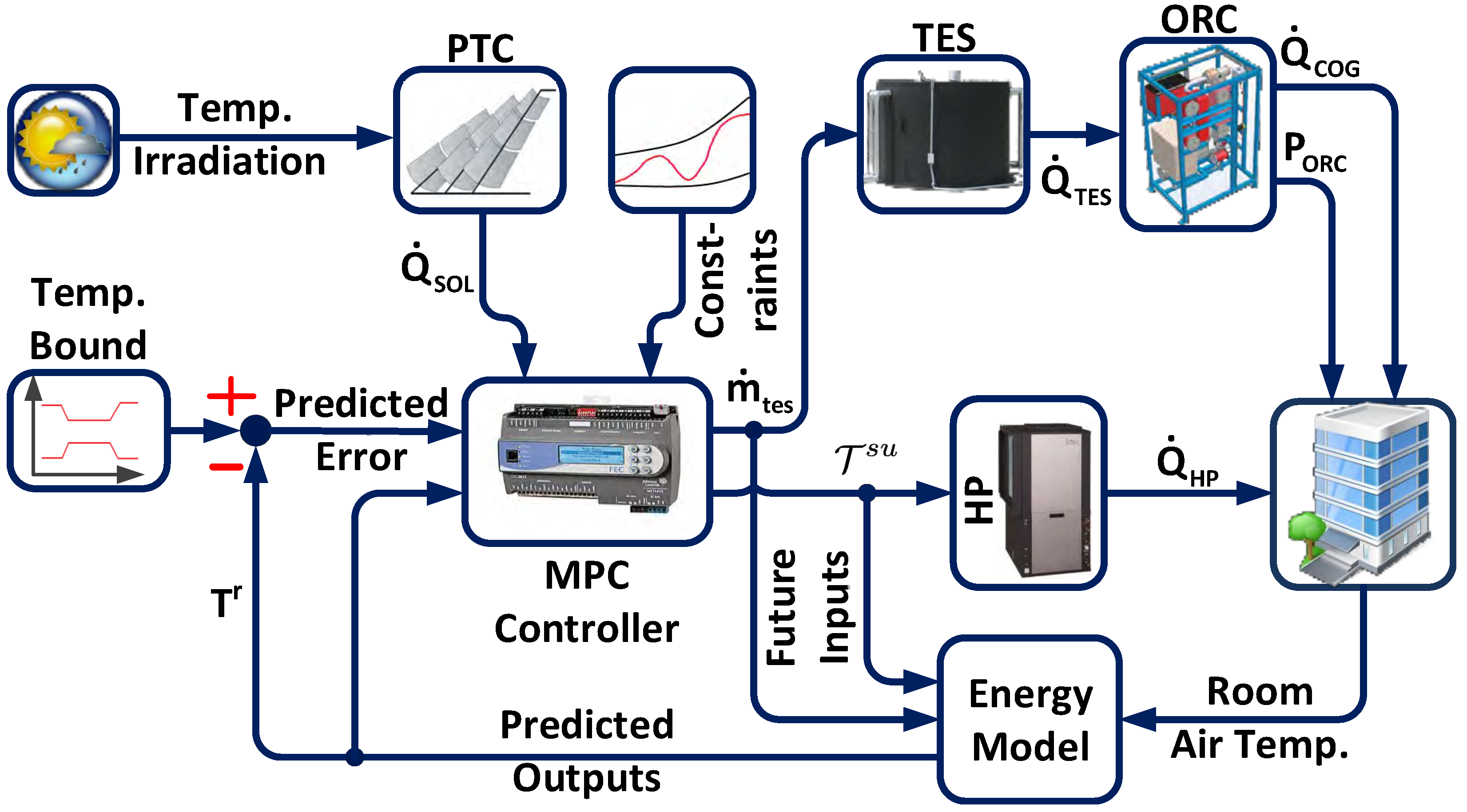
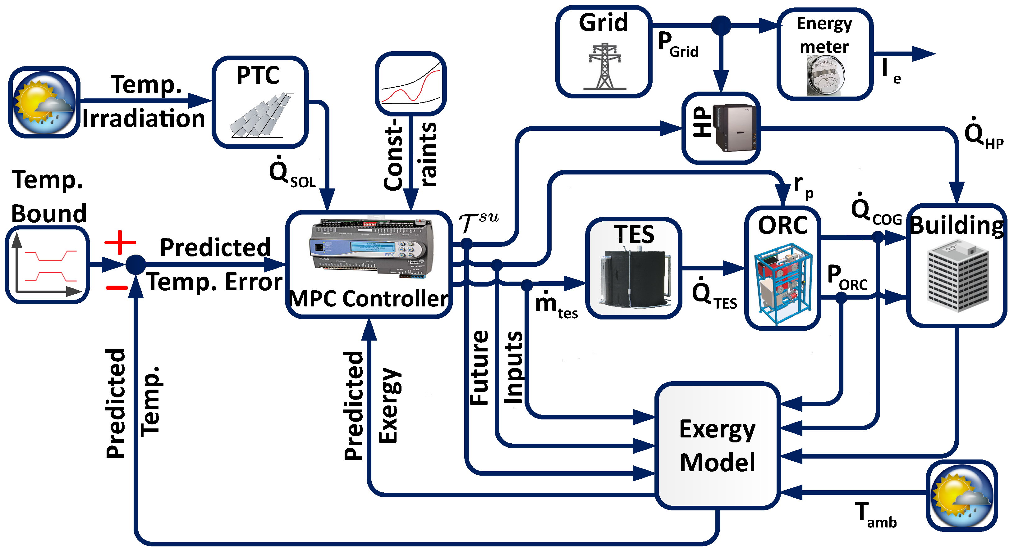
5.1. Control Structure

In this section, the structure of the designed MPCs for a common heating application (Architecture (a) in Figure 6) of the combined MicroCSP and building HVAC system is discussed for a same building testbed. Lakeshore Center building at Michigan Technological University is the testbed utilized in all our prior studies in [16,17,18,19,20,21,22]; thus, it is briefly explained here. This is an office building with three floors. Each individual office room is considered as a thermal zone. The thermal zone is heated in three stages (Figure 13):

• In the air handling unit (AHU), air from the outside is preheated by exchanging energy with return air from the thermal zone in the energy recovery ventilator (ERV).
• In the MicroCSP, solar energy is converted to low-grade thermal energy (${\dot{Q}}_{COG}$) and electricity ($P_{ORC}$). The preheated air in the AHU is further heated by the low-grade thermal energy from the ORC.
• The Heat pump (HP) further heats the air from the AHU to the thermal zone by using electricity from the ORC and/or from the power grid.

5.1.1. Building Energy Management

The energy of the building can be optimized by using the first and/or second law of thermodynamics. The first law of thermodynamics encapsulates the energy usage and the energy conversion efficiency of the system. The second law of thermodynamics encapsulates the quality of different forms of energy (solar energy, thermal energy, electricity, etc.) in a given environment. The second law of thermodynamics further differentiates the total input energy into the available energy, known as exergy, and unavailable energy. In tune with that, the structure of the designed MPCs based on the first and second laws of thermodynamics are discussed in this section. The MPCs designed by applying the first and second laws of thermodynamics are termed as the energy-based MPC (EMPC) and exergy-based MPC (XMPC), respectively. In addition to MPCs, the structure of the designed adaptive neuro-fuzzy inference system (ANFIS) controller trained by EMPC data is discussed. The ANFIS controller is designed as a compromise between optimality and computational effort of the controller.

5.1.1.1. Energy-Based Model Predictive Controller (EMPC)

Figure 14 shows the structure of an EMPC [18,20] designed for the combined MicroCSP and building HVAC system. The designed EMPC maintains the temperature ($T^r$) of each room of the building within the ASHRAE specified upper and lower comfort temperature bounds (${\overline{T}}_t^r$ and ${\underline{T}}_t^r$), respectively, by minimizing the electrical energy usage of the building.

Equation (18) shows the electrical energy usage ($E_b$) of the building HVAC system. $P^H$ and $P^F$ are calculated using Equations (12) and (13), respectively.

$$\begin{array}{c}\hfill E_b=\sum _{t=0}^{t_f}[(P^H\left[t\right]+P^F\left[t\right])·\Delta t]\end{array}$$

(18)

The electrical energy consumption of the combined MicroCSP and building HVAC system ($E_{Sys}$) is calculated as shown in Equation (19).

$$\begin{array}{c}\hfill E_{Sys}=E_b-\sum _{t=0}^{t_f}(P_{ORC}\left[t\right]·\Delta t)\end{array}$$

(19)

At any given time (t), the HVAC fan power consumption ($P^F$) is assumed to be constant for the testbed studied, whereas the HVAC power consumption ($P^H$) is proportional to ${\mathcal{T}}^{su}$ (Equation (12)), and the electrical power from the ORC ($P_{ORC}$) is a function of ${\dot{m}}_{tes}$ according to Equation (11).

The designed EMPC minimizes the electrical energy usage of the building by optimizing the HP supply temperature (${\mathcal{T}}^{su}$), and the mass flow rate of TES fluid (${\dot{m}}_{tes}$) at the current time (t) and future time ($t+k)$ by utilizing the ambient temperature and solar irradiation predictions, and the ASHRAE specified temperature bound. The ambient temperature and solar irradiation forecast data can be obtained from commercial organizations like Solcast [99]. Furthermore, the designed EMPC is bound by constraints and manufacturer specified limits. In the designed EMPC, soft constraints are used by adding slack variables ($\overline{ϵ}$ and $\underline{ϵ}$) and multiplying the slack variables by a weight factor (${\rho }_{wt}$) to be minimized while ensuring optimal solution at all times. The objective function of the designed EMPC is detailed in Equation (20) subject to the constraints in Equation (21).

$$\begin{array}{cc}\hfill & \underset{{\dot{m}}_{tes},{\mathcal{T}}^{su},\overline{ϵ},\underline{ϵ}}{\min }\{E_{Sys}+{\rho }_{wt}·\left(\right|\overline{ϵ}|+|\underline{ϵ}\left|\right)\}\hfill \end{array}$$

(20)

Subject to the following constraints:

$$\begin{array}{cc}\hfill & T_{t+k+1|t}=A{T}_{t+k|t}+B{\mathcal{T}}_{t+k|t}^{su}+E{d}_{t+k|t}\hfill \end{array}$$

(21a)

$$\begin{array}{cc}& T_{t+k|t}^z=C{T}_{t+k|t}\hfill \end{array}$$

(21b)

$$\begin{array}{cc}& P_{ORC,t+k|t}=f({\dot{m}}_{{tes}_{t+k|t}})\hfill \end{array}$$

(21c)

$$\begin{array}{cc}& {\dot{Q}}_{COG,t+k|t}=g({\dot{m}}_{{tes}_{t+k|t}})\hfill \end{array}$$

(21d)

$$\begin{array}{cc}& SO{C}_{t+k+1|t}^{TES}=SO{C}_{t+k|t}^{TES}+{\displaystyle \frac{{\sum }_{t+k|t}^{t+k+1|t}({\dot{Q}}_{SO{L}_{t+k|t}}-{\dot{Q}}_{{TES}_{t+k|t}}).\Delta t}{C_{TES}}}\hfill \end{array}$$

(21e)

$$\begin{array}{cc}& SO{C}_1^{TES}=SO{C}_{t_{max}}^{TES}\hfill \end{array}$$

(21f)

$$\begin{array}{cc}& {\underline{SOC}}^{TES}\le SO{C}_{t+k+1|t}^{TES}\le {\overline{SOC}}^{TES}\hfill \end{array}$$

(21g)

$$\begin{array}{cc}& 0\le {\dot{m}}_{{tes}_{t+k|t}}\le {\dot{m}}_{max}\hfill \end{array}$$

(21h)

$$\begin{array}{cc}& T_{t+k|t}^{HP}\le {\mathcal{T}}_{t+k|t}^{su}\le {\overline{\mathcal{T}}}_{t+k|t}\hfill \end{array}$$

(21i)

$$\begin{array}{cc}& {\underline{T}}_{t+k|t}^r-{\underline{ϵ}}_{t+k|t}\le T_{t+k|t}^r\le {\overline{T}}_{t+k|t}^r+{\overline{ϵ}}_{t+k|t}\hfill \end{array}$$

(21j)

$$\begin{array}{cc}& {\underline{ϵ}}_{t+k|t},{\overline{ϵ}}_{t+k|t}\ge 0\hfill \end{array}$$

(21k)

The thermal dynamics of the building rooms are captured by the equality constraints in the state-space Equations (21a) and (21b); the ORC model is included in Equations (21c) and (21d); SOC of the TES is estimated in Equation (21e); Equation (21f) presents the charge sustaining constraints of the TES; Equation (21g) bounds the SOC of the TES within the lower and upper bounds set to 5% and 95%, respectively; Equation (21h) is the maximum HTF mass flow rate (${\dot{m}}_{max}$) dictated by the ORC manufacturer [100]; Equation (21i) shows the constraints on the supply air temperature that also represents the constraint on the control input; Equation (21j) defines the temperature bounds of the thermal zone temperature and includes the slack variables that relaxes this constraint to add flexibility and guarantee the existence of a solution of the optimization; and, finally, Equation (21k) enforces that the slack variables are always positive.

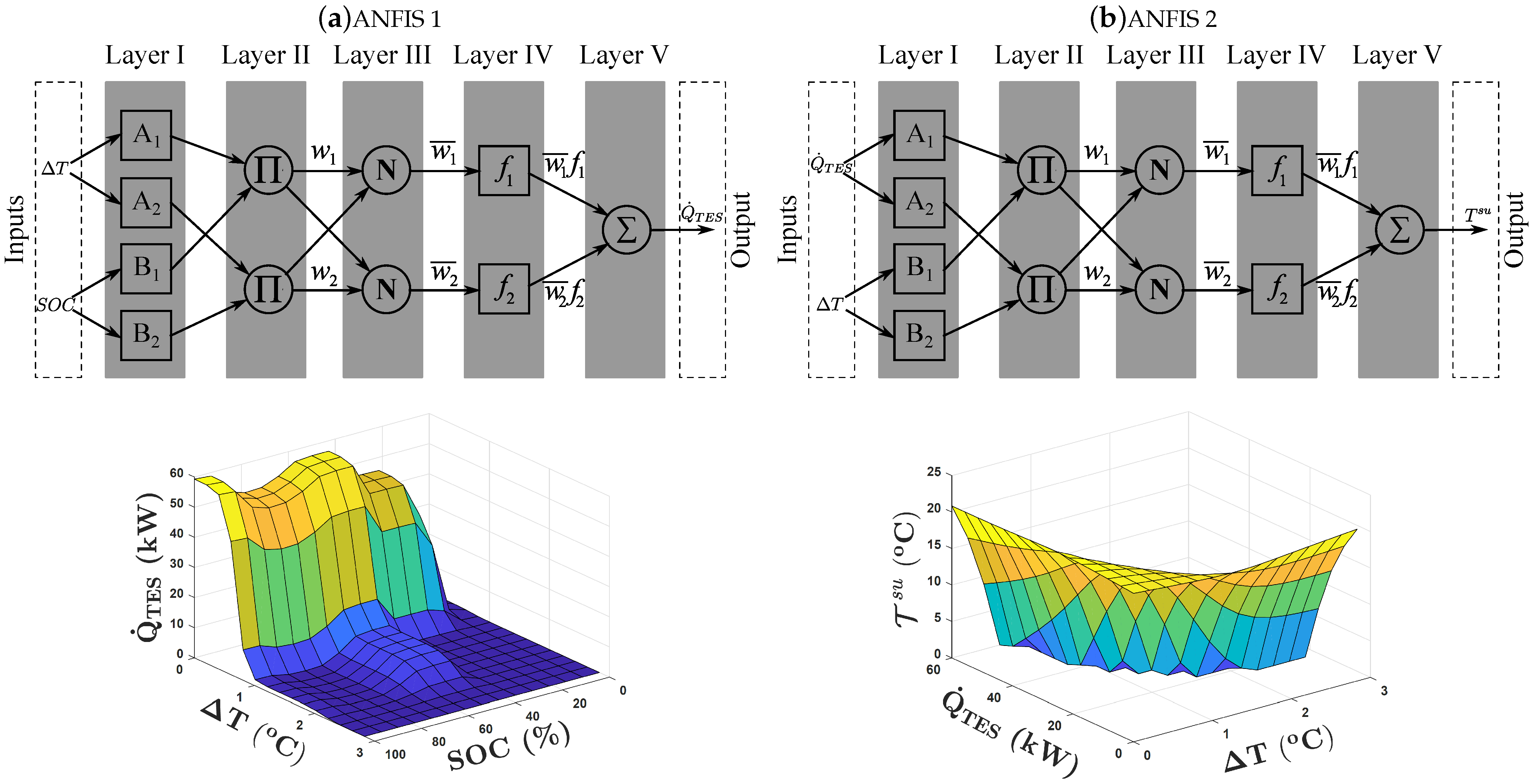
• Offline EMPC-Trained Adaptive Neuro-Fuzzy Inference System (ANFIS) Controller

The designed EMPC is computationally expensive and is not easily implementable in low-cost HVAC controllers currently available in the market. To mitigate this problem, we proposed in [19] an adaptive neuro-fuzzy inference system (ANFIS) controller. The designed ANFIS controller is computationally inexpensive and easily implementable since it is rule-based and capable of approximating nonlinear functions.

The designed ANFIS controller consists of two cascaded ANFIS models acting one after the other. Each ANFIS model consists of a five-layer artificial neural network (Figure 15) that is trained offline using data from the EMPC (Figure 14) for a broad operating range of the building. The first ANFIS model is fed by the temperature difference ($\Delta T$) between the room temperature and the lower comfort temperature bound, and the SOC of the TES. The output of the first ANFIS model is the thermal power dispatched from the TES (${\dot{Q}}_{TES}$). Then, the second ANFIS model takes the thermal power dispatched from the TES as an input along with the difference between the room temperature and the lower comfort temperature bound. Finally, the designed ANFIS controller commands the required supply temperature (${\mathcal{T}}^{su}$) by deciding the quantity of heat needed from the HP to ensure that the room air temperature is within the comfort temperature bounds.

5.1.1.2. Exergy-Based Model Predictive Controller (XMPC)

Exergy analysis provides much more insight than energy analysis for the control of a system to maximize the efficiency in a particular environment [101]. Exergy analysis can determine the loss of work potential (i.e., exergy destruction) during a process, which is caused by the irreversibilities and entropy production in a system [102]. Hence, the optimality of the designed exergy-based MPC (XMPC) [21,22] is determined by the exergy saving of the combined HVAC and MicroCSP system in a building.

Figure 16 shows the structure of the designed XMPC for the combined MicroCSP and HVAC system. The designed XMPC maintains the temperature ($T^r$) of each room in the building within the specified upper and lower comfort temperature bounds (${\overline{T}}_t^r$ and ${\underline{T}}_t^r$) by maximizing the second law efficiency of the combined MicroCSP and building HVAC system.

Equation (22) shows that reducing the exergy destruction (${\dot{X}}_{dest}$) or increasing the exergy recovered (${\dot{X}}_{rec}$) for a given supplied exergy (${\dot{X}}_{sup}$) will increase the second law efficiency (${\eta }_{II}$) of the system.

$$\begin{array}{ccc}\hfill {\eta }_{II}=& \frac{{\dot{X}}_{rec}}{{\dot{X}}_{sup}}=\hfill & \hfill 1-\frac{{\dot{X}}_{dest}}{{\dot{X}}_{sup}}\end{array}$$

(22)

Equation (23) evaluates the exergy destruction in the building (${\dot{X}}_{dest}^b$) assuming that all the building rooms are flowing control volumes. Minimizing the exergy destruction in the building (${\dot{X}}_{dest}^b$) minimizes the energy usage of the building accounting for the ambient conditions. Finally, Equation (24) shows that exergy recovered in the ORC (${\dot{X}}_{rec}^{ORC}$) is a function of the mass flow rate of TES fluid (${\dot{m}}_{tes}$) and the operating pressure ratio ($r_p$) of the ORC.

$$\begin{array}{cc}\hfill {\dot{X}}_{dest}^b\left[t\right]=& \sum _{i\in N_i^r}(\left[\sum _{j\in N_i^r}(1-\frac{T_{amb}\left[t\right]}{T_i^r\left[t\right]})(\frac{T_j^r\left[t\right]-T_i^r\left[t\right]}{R_{i,j}^w})\right]\hfill \\ \hfill & +{\dot{m}}_i^r\left[t\right]·\left[c_{p,air}·({\mathcal{T}}_i^{su}\left[t\right]-T_i^r\left[t\right])-T_{amb}\left[t\right]·c_{v,air}·ln(\frac{{\mathcal{T}}_i^{su}\left[t\right]}{T_i^r\left[t\right]})\right]\hfill \\ \hfill & -\frac{m_i^{room}·c_{v,air}}{t_{sample}}·\left[(T_i^r\left[t\right]-T_i^r[t-1])-T_{amb}\left[t\right]·ln\frac{T_i^r\left[t\right]}{T_i^r[t-1]}\right])\hfill \end{array}$$

(23)

$$\begin{array}{cc}\hfill {\dot{X}}_{rec}^{ORC}\left[t\right]=& f({\dot{m}}_{tes}\left[t\right],r_p\left[t\right])\hfill \end{array}$$

(24)

Equation (25) shows the objective function of the XMPC designed to maximize the second law efficiency of the combined MicroCSP and building HVAC system.

$$\begin{array}{c}\hfill \underset{{\mathcal{T}}^{su},r_p,{\dot{m}}_{tes},\overline{ϵ},\underline{ϵ}}{\min }\{{\dot{X}}_{dest}^b-{\dot{X}}_{rec}^{ORC}+{\rho }_{wt}·\left(\right|\overline{ϵ}|+|\underline{ϵ}\left|\right)\}\end{array}$$

(25)

The designed XMPC optimizes the HP supply temperature (${\mathcal{T}}^{su}$), $r_p$, and ${\dot{m}}_{tes}$ at the current time (t) and future time ($t+k)$ knowing the ambient temperature, solar irradiation, and temperature bound predictions. However, the designed XMPC actuates the TES, ORC, and HP at the current time (t). The designed XMPC uses soft constraints ($\overline{ϵ}$ and $\underline{ϵ}$) to ensure optimal solution at all times. The designed XMPC is subject to the exergy related equality constraints in Equation (26) along with the constraints previously listed in Equation (21).

$$\begin{array}{c}\hfill \begin{array}{cc}\hfill {\dot{X}}_{des{t}_{t+k|t}}^b=& \sum _{i\in N_i^r}\{\sum _{j\in N_i^r}(1-\frac{T_{am{b}_{t+k|t}}}{T_{i_{t+k|t}}^r})(\frac{T_{j_{t+k|t}}^r-T_{i_{t+k|t}}^r}{R_{i,j}^w})\hfill \\ \hfill & +{\dot{m}}_{i_{t+k|t}}^r·[c_{p,air}·({\mathcal{T}}_{i_{t+k|t}}^{su}-T_{i_{t+k|t}}^r)-T_{am{b}_{t+k|t}}·c_{v,air}·ln(\frac{{\mathcal{T}}_{i_{t+k|t}}^{su}}{T_{i_{t+k|t}}^r})]\hfill \\ \hfill & -\frac{m_i^{room}·c_{v,air}}{t_{sample}}·[(T_{i_{t+k|t}}^r-T_{i_{t+(k-1)|t}}^r-T_{am{b}_{t+k|t}}·ln\frac{T_{i_{t+k|t}}^r}{T_{i_{t+(k-1)|t}}^r}]\}\hfill \end{array}\end{array}$$

(26a)

$$\begin{array}{cc}\hfill {\dot{X}}_{re{c}_{t+k|t}}^{ORC}=& f({\dot{m}}_{te{s}_{t+k|t}},r_{p_{t+k|t}})\hfill \end{array}$$

(26b)

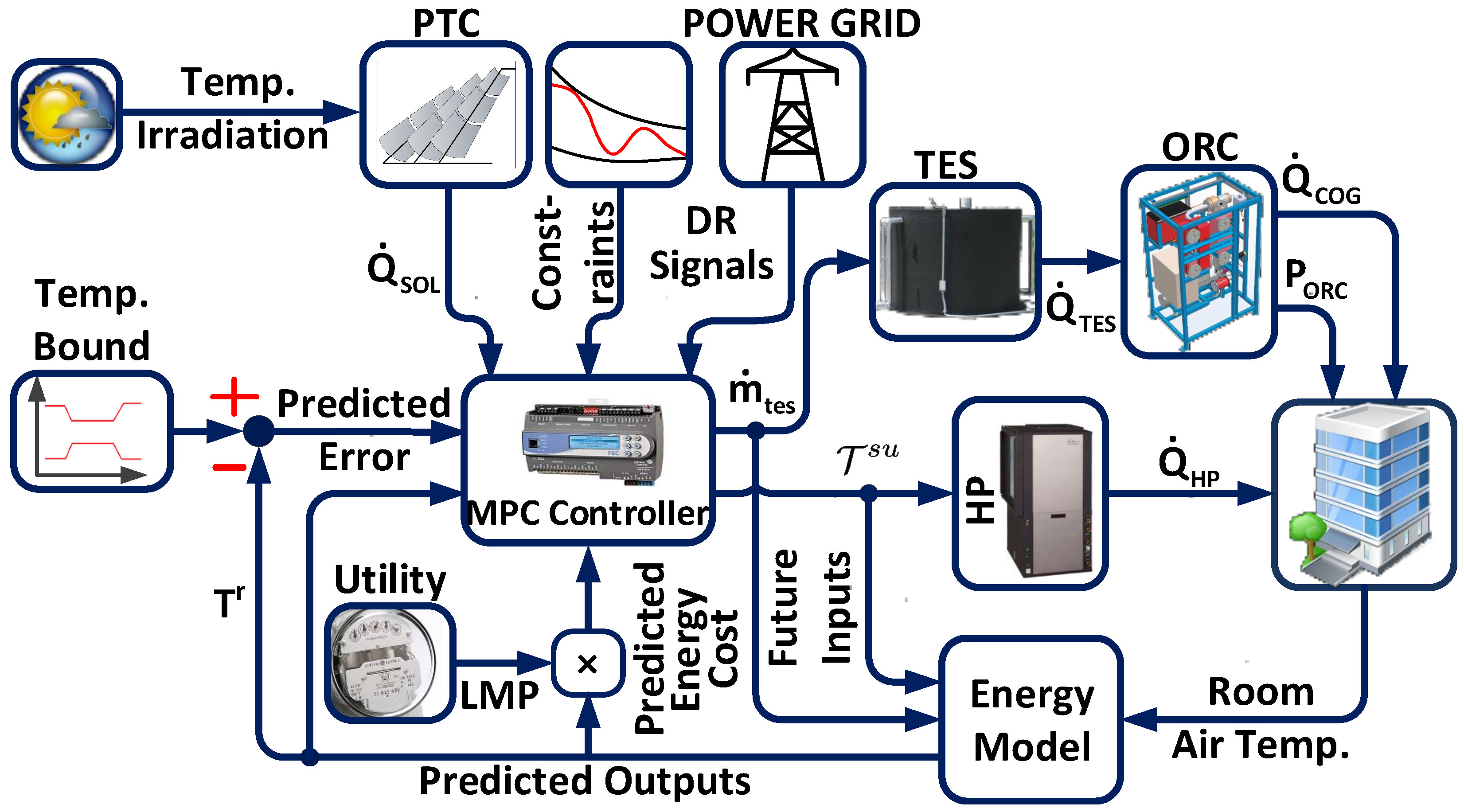
5.1.2. Energy Cost-Based Model Predictive Controller (CMPC)

The designed EMPC in Section 5.1.1.1 minimizes the energy usage of the combined MicroCSP and building HVAC system. Furthermore, the designed EMPC also minimizes the electrical energy cost when the price of electrical energy is fixed during a day. However, EMPC needs to be re-designed to minimize the electrical energy cost of the combined MicroCSP and building HVAC system when the price of electrical energy is dynamic and changes during a day. To this end, in our prior works [17,20], we designed variants of the energy cost-based MPCs (CMPCs) for the combined MicroCSP and building HVAC systems. Figure 17 shows the structure of the designed CMPC. The designed CMPC minimizes the electrical energy cost of the building HVAC and MicroCSP system while maintaining the temperature of the thermal zone within the specified comfort temperature bounds.

The electrical energy cost is calculated as the product of the locational marginal price (${\Omega }_t$) of electricity and the electrical energy consumed by the combined MicroCSP and building HVAC system ($E_{Sys}$). Section 5.1.1.1 shows that the electrical energy consumption of the combined MicroCSP and building HVAC system ($E_{Sys}$) is controlled by the HP supply temperature (${\mathcal{T}}^{su}$) and the mass flow rate of TES fluid (${\dot{m}}_{tes}$). In tune with that, the objective function of the designed CMPC is given in Equation (27), subject to the same constraints previously listed in Equation (21).

$$\begin{array}{cc}\hfill & \underset{{\dot{m}}_{tes},{\mathcal{T}}^{su},\overline{ϵ},\underline{ϵ}}{\min }\{E_{Sys}·{\Omega }_t+{\rho }_{wt}·\left(\right|\overline{ϵ}|+|\underline{ϵ}\left|\right)\}\hfill \end{array}$$

(27)

5.1.3. Building to Grid Demand Response Model Predictive Controller (DRMPC)

Building HVAC systems combined with MicroCSP have great potential to provide ancillary services to support the power grid and participate in the demand response (DR) programs by readjusting their consumption. Our prior work [16] discusses a building to grid demand response MPC (DRMPC) that shows the effect of incentives on the participation of the building to the DR program and its allegiance to the requested DR load.

Figure 18 shows the structure of the designed DRMPC to maintain the room temperature within the comfort temperature bounds while minimizing the HVAC and MicroCSP electrical energy cost by considering the DR incentive ($\Theta$) from the grid operator. The objective function of the designed DRMPC is provided in Equation (28):

$$\begin{array}{c}\hfill \underset{{\mathcal{T}}^{su},{\dot{m}}_{tes},\underline{ϵ},\overline{ϵ}}{\min }\left(E_{Sys}·({\Omega }_t-{\Theta }_t)+{\rho }_{wt}·\left(\right|\underline{ϵ}|+|\overline{ϵ}\left|\right)\right)\end{array}$$

(28)

The optimization problem is subject to the constraints listed in Equation (21) along with the grid power limitation constraint in Equation (29):

$$\begin{array}{c}\hfill P_{Sy{s}_{t+k|t}}\le P_{Gri{d}_{t+k}}\end{array}$$

(29)

While the objective function ensures that the building will consume more energy when the DR incentive is sent by the grid operator, the constraint of Equation (29) guarantees that the building power consumption ($P_{Sys}$) is always less than or equal to the maximum allowable building power consumption from the grid ($P_{Grid}$).

In Equation (28), the electrical energy cost of the combined MicroCSP and building HVAC system is modified from CMPC in Section 5.1.2 to take advantage of $\Theta$ from the grid operator. Furthermore, Section 5.1.1.1 shows that $E_{Sys}$ is controlled by ${\mathcal{T}}^{su}$, and ${\dot{m}}_{tes}$. Finally, Equation (28) uses soft constraints ($\underline{ϵ}$ and $\overline{ϵ}$) to ensure feasibility of the solution at all times.

5.2. Control Results

The controllers in Section 5.1 are implemented for the testbed in Figure 13. Here, the results from our previous studies [16,19,20,21] for the same testbed are discussed. To provide a fair comparison among different control methods, the results are presented for a same sunny winter day (Figure 19) considering 72 rooms (thermal zones), a prediction horizon of 24 h, and a 30 min time step. Note that the optimizations were performed through the Yalmip toolbox [103] in MATLAB^® using an open-source solver IPOPT [104] and a commercial solver Gurobi [105].

The baseline rule-based controller (RBC) has the following rules to determine supply air temperature by the HP:

• The HP is switched off if the room air temperature is above the upper limit for the desired air temperature of the room (${\overline{T}}_{i,t}^r$).
• The HP is switched on to its maximum capacity (${\mathcal{T}}_{i,t}^{su}$ = ${\overline{T}}_{i,t}$) if the room air temperature is below the lower limit for desired air temperature of the room (${\underline{T}}_{i,t}^r$).
• If the room air temperature is between the upper and lower limits for the desired air temperature of the room, then, to avoid chattering of HP, the HP is switched Off or On depending on the HP status at the previous time step.

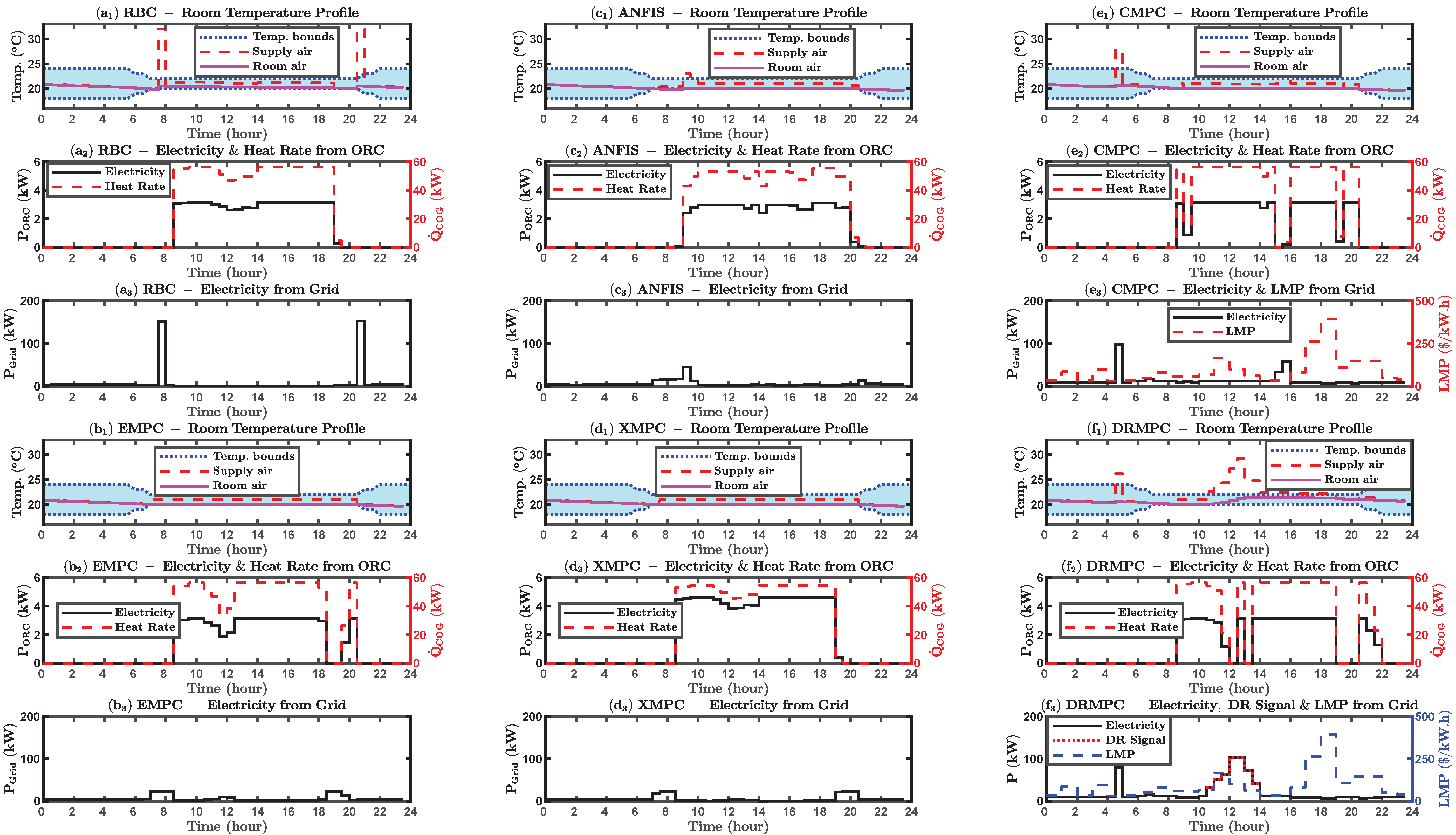
Figure 20 shows the control results of the combined MicroCSP and building HVAC system when the baseline RBC, EMPC, ANFIS controller, XMPC, CMPC, and DRMPC are applied. In Figure 20, each section consists of three subplots:

(i)

Room air temperature profile, HP supply air temperature, and ASHRAE temperature comfort bound based on room occupancy

(ii)

Heat flow rate and electrical power from the ORC

(iii)

Consumed electricity power, localized marginal pricing (LMP), and/or DR signal from the grid

The performance of each controller in Figure 20 is discussed in the following.

RBC: 

The room air temperature in Figure 20a${}_1$ starts at 21 °C and ramps down until it reaches below the lower temperature bound. Then, the HP is switched on to its maximum capacity to increase the room air temperature. From 8:30 AM to 7:30 PM, the heat rate from MicroCSP through the ORC maintains the room air temperature within the bounds, while the HP is switched off. The electricity and heat rate from the ORC are shown in Figure 20a${}_2$. Electricity from the ORC is used to aid the electrical consumption of the HVAC fan in the room. At 7:30 PM, the solar energy production ceases for the day and the heat rate from the TES is fully utilized by the ORC. Hence, the room air temperature ramps down from 7:30 PM until it reaches below the lower temperature bound at about 8:30 PM. When the room air temperature reaches below the lower temperature bound, the HP switches on again to its maximum capacity. Figure 20a${}_3$ shows the power consumed by the HP from the grid.

EMPC: 

This optimal controller predicts room air temperature and available solar thermal energy via ORC; thus, it predicts when the room air temperature is about to violate the lower temperature bound and supplies the minimum amount of energy required for the HP to maintain the room air temperature at the lower temperature bound. In addition, EMPC controls the TES to optimally store the heat from the PTC and supply it to the ORC. From 8:30 AM to 6:30 PM and from 7:30 to 8:30 PM, the heat rate from ORC maintains the room air temperature within the temperature bounds, while the HP is switched off. The electrical power and heat flow rate from the ORC are shown in Figure 20b${}_2$. Electricity from the ORC is used to aid the electrical consumption of the HVAC fan in the room. After 8:30 PM, the room air temperature ramps down until the end of the day. Compared to Figure 20a${}_3$, Figure 20b${}_3$ shows much less electrical power consumed by the HP from the grid.

ANFIS: 

ANFIS controller is a rule-based controller trained by the optimal EMPC. Therefore, the ANFIS controller tries to mimic optimal EMPC but does not have the capability to predict like EMPC. In tune with that, Figure 20c${}_1$ shows that the room air temperature is maintained near the lower temperature bound. From 7:00 AM to 8:30 PM, unlike EMPC, the room air temperature is not always at the lower temperature bound but the room air temperature goes above and below the lower temperature bound. In addition, by comparing Figure 20a${}_1$,c${}_1$, it can be seen that the magnitude of the room air temperature violations is reduced when we move from RBC to ANFIS controller. This is because RBC does not undergo training and mainly acts on current measured room temperature and previous control actions but the ANFIS controller is trained by the optimal EMPC. Figure 20c${}_2$ shows that the ORC is operational from 9:00 AM to 8:30 PM, and the heat rate from ORC maintains the room air temperature within the temperature bounds, while the electricity from the ORC is used to aid the electrical consumption of the HVAC fan in the room.

XMPC: 

Figure 20d${}_1$ shows the room air temperature when the optimal XMPC is applied to the combined MicroCSP and building HVAC system. XMPC minimizes the exergy destruction in the room and maximizes the exergy recovered in the ORC. Hence, XMPC adds the minimum amount of heat to the room such that the exergy destruction of the room is minimum. Additionally, XMPC operates the ORC at the optimal pressure ratio ($r_p$) so that the exergy recovered from the ORC is maximized. HP supplies the heat to the room from 7:00 AM to 8:30 AM and from 7:00 PM to 8:30 PM, when there is no availability of any solar thermal energy. This is reflected in the grid power consumption shown in Figure 20d${}_3$. However, Figure 20d${}_2$ shows that from 8:30 AM to 7:00 PM the heat rate from ORC maintains the room air temperature within the temperature bounds, while the electrical power from the ORC supplies the HVAC fan in the room.

CMPC: 

Figure 20e${}_1$ depicts the profiles of the room air temperature and the supply air temperature within the comfort temperature bounds. Based on the predictions of the LMP of electricity from the power grid (Figure 20e${}_3$), the CMPC preheats the room during the non-occupancy period, around 4:30 AM when electricity is cheaper, to ensure that the room air temperature never violates the temperature bounds, and the energy cost of heating the room is minimized. During the occupancy period, the CMPC provides just the amount of heat, through the supply air, to keep the room air temperature at the lower bound reducing the cost of energy. The CMPC controls the TES to optimally store the heat from the PTC and supply it to the ORC when needed. As shown in Figure 20e${}_2$, the cogenerated heat is supplied to the room from 8:30 AM to 3:00 PM and from 3:30 to 8:30 PM to avoid running the HP with electricity since the LMP is high during this period. The HP is only turned on when the LMP is cheap around 3 PM as reflected by the power consumed from the grid in Figure 20e${}_3$.

DRMPC: 

DRMPC seeks to minimize its energy cost of the building and increase its profit by contributing to the load following DR program. This means that the building should consume extra energy to follow the DR load dictated by the grid operator. Hence, an optimal incentive, $\Theta$ = 180$/MWh in this case, must be provided by the grid operator to compensate for the extra energy cost [16]. Figure 20f${}_1$ shows that, although the room air temperature is inside the comfort bounds, the DRMPC turns on the HP at 4:30 AM when the LMP is low (Figure 20f${}_3$), to prevent temperature violation. During the occupancy period, the DRMPC reduces the HVAC energy consumption by supplying the necessary heat to keep the room air temperature at the lower temperature bound from 7 AM until the DR signal is received at 10:30 AM (Figure 20f${}_3$). From that time, the room air temperature starts increasing since the building is providing DR by consuming electricity in the HP, as shown in Figure 20f${}_3$. The electricity and heat cogeneration of the ORC are depicted in Figure 20f${}_3$.

The total energy consumption and energy cost of the building for the results in Figure 20 are provided in

Table 4. Comparison of the different control frameworks on energy consumption and the HVAC electrical energy cost for a sample day (18 March 2016).

Control	Energy Consumption [kWh/Day]	Energy Saving * [%]	Energy Cost Consumption [$/Day]	Cost Saving * [%]
RBC [20]	208.7	-	21.5	-
EMPC [20]	130.3	37.7	13.6	36.7
ANFIS ${}^{\#}$ [19]	138.5	33.6	17.3	19.5
XMPC [21]	114.1	45.3	12.4	42.3
CMPC [20]	134.3	35.6	6.4	70.2
DRMPC [16]	467.7	−124.1	0.2	99.1

* Percentages are calculated by comparing with the baseline RBC. ^# Computational time of the ANFIS controller reduces by 90% in comparison with the EMPC.

for comparing the six controllers. The following information is obtained from the data in Table 4.

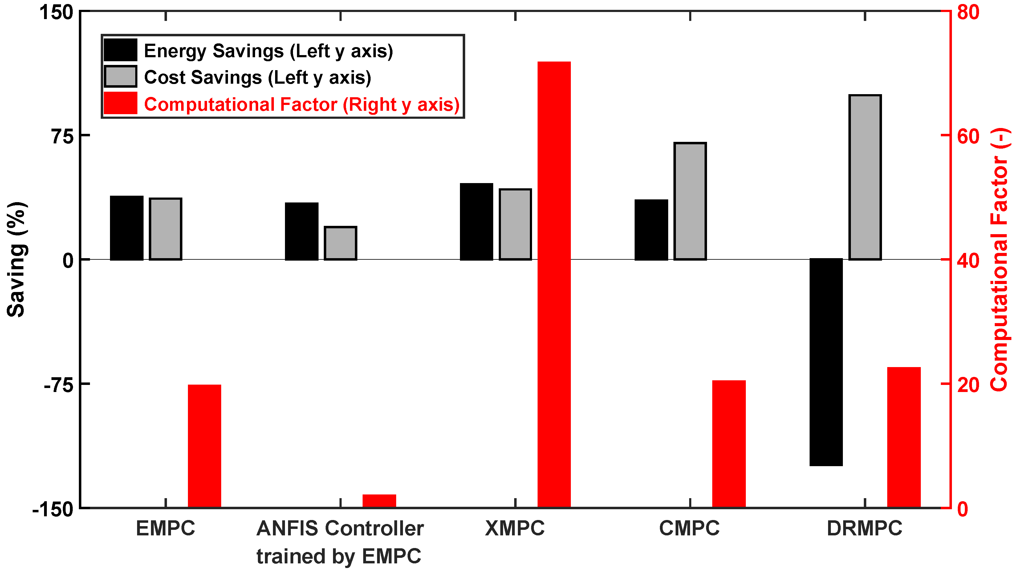
• By changing the controller from RBC to EMPC, the energy usage of the building is reduced by 38%.

• By changing the controller from RBC to ANFIS controller (trained by EMPC data for a broad building operating range), the energy usage of the building is reduced by 34%. However, the energy usage is 4% higher than when optimal EMPC is used. However, the trade-off achieved is a 90% reduction in computational cost, which enables implementation in low-cost HVAC controllers.

• By changing the controller from RBC to XMPC, the energy usage of the building is reduced by 45%. The energy usage of the building of XMPC reduces by 7%, compared to EMPC. This is because EMPC optimally coordinates the HP and the MicroCSP to reduce the quantity of energy used by the building, while XMPC maximizes the availability of the energy to the building in specified ambient conditions.

• By changing the controller from RBC to CMPC, the electrical energy cost of the building is reduced by 70%. The reduction in the electrical energy cost of the building when CMPC is used is higher than when EMPC, ANFIS controller, or XMPC is used. This is because, EMPC, ANFIS controller, and XMPC do not consider LMP in their objective functions.

• By changing the controller from RBC to DRMPC, the energy cost of the building is reduced by optimally coordinating the HP and MicroCSP while considering the LMP and DR incentive. Furthermore, Table 4 shows that, when DRMPC is applied, the energy consumption of the building is maximum (increases by 124%, compared to RBC) and the energy cost of the building is minimum (decreases by 99%, compared to RBC). This is because the objective function of DRMPC is formulated so that the energy usage of the building is maximized when the grid shows low LMP and/or shows a high DR incentive.

The results in Table 4 do not account for the prediction uncertainties of the weather conditions, the solar irradiation, and the LMP. Thus, they can be subject to interpretation. Our previous works in [17,18,19,20,21] also quantify the range of energy and electrical energy cost savings of the combined MicroCSP and building HVAC system by considering the prediction uncertainties of the controller inputs and performing Monte-Carlo simulations (MCS). The prediction uncertainties are generated by adding a white noise with a signal-to-noise ratio of 5 dB to the controller inputs, namely the ambient temperature, the solar irradiation, and the LMP, for the sample day (Figure 19).

Figure 21 shows sample MCS results performed using at least one hundred randomly generated controller inputs. Figure 21a depicts the probability distribution of the energy savings of the combined MicroCSP and building HVAC system by applying EMPC, compared to using RBC. Additionally, Figure 21b depicts the probability distribution of electricity cost savings when CMPC is applied to the combined MicroCSP and building HVAC system, compared to when RBC is applied. Figure 21 shows that the energy savings is at least 37% and the cost savings is at least 70% for more than half of the instances. In addition, Figure 21 shows that the building energy-saving and cost saving will always be above 33% and 68%, respectively. Finally,

Table 5. Summary of the Monte-Carlo simulation results of the different control frameworks by considering prediction uncertainties.

Control Type	Range	Mean	Standard Deviation
	Energy Saving [%] *
EMPC [20]	33.5–41.5	37.5	2.5
ANFIS [19]	26.5–37	33	3.4
XMPC [21]	44–46.5	45	0.7
	Cost Saving [%] *
CMPC [20]	68.5–71.5	70	0.9

* Percentages are calculated by comparing with the baseline RBC.

shows the range, mean, and standard deviation of the building energy or cost savings when we change from the baseline RBC to the designed optimal controllers.

6. Summary and Recommendations for Future Directions

6.1. Summary

This paper presents an overview of optimal integration and control of micro-scale concentrated solar power (MicroCSP) systems (i.e., rated power < 1 MW) into the building heating, ventilation, and air-conditioning (HVAC) system. This integration requires well-designed control strategies in order to fully exploit the additional degrees of freedom offered by the MicroCSP. The rule-based controller (RBC) is the simplest and most used control technique for HVAC systems in buildings. It is based on a pre-determined set of rules that are implemented to control the behavior of a system. However, due to the complexity of the building HVAC system in tandem with MicroCSP, the development of optimal rules for the RBC to control this system is challenging. In fact, the RBC, in this case, should be able to consider not only the temperatures of the building rooms but also the state of charge (SOC) of the thermal energy storage (TES) system, the solar field production, and the power engine efficiency, as well as the uncertainties related to each one of these components.

This paper looks at various optimal control strategies applied to the combined MicroCSP and building HVAC system. Figure 22 shows the summary of control results of the designed optimal controllers compared to RBC. The building energy savings reduce by 38% when an energy-based model predictive controller (EMPC) is applied to the combined MicroCSP and building HVAC system instead of using the RBC. Furthermore, by implementing EMPC trained adaptive fuzzy-neuro inference system (ANFIS) controller, a compromise between building energy savings and the computational factor is utilized. The building energy savings by the ANFIS controller reduces by 4% but the computational factor decreases by 73%, compared to that in the EMPC.

The exergy-based model predictive controller (XMPC) reduces the building energy savings by 45%, compared to when RBC is applied. Furthermore, XMPC shows the maximum building energy savings; however, the highly nonlinear exergy functions make XMPC the most computational expensive among the optimal controllers discussed.

The control frameworks of the energy cost-based model predictive controller (CMPC) and the building to grid demand response model predictive controller (DRMPC) are designed to reduce the building energy cost when the combined MicroCSP and building HVAC system is connected to a power grid. The application of CMPC reduces the building energy cost by 70%, compared to that in the RBC. This cost-saving is increased to 99% when DRMPC is used by taking advantage of grid incentives to accommodate DR requests by the grid.

Monte-Carlo simulation (MCS) results show that moving from RBC to XMPC guarantees the lowest variations in building energy savings among the five designed controllers. In addition, MCS results show that the ANFIS controller, which is trained offline and cannot optimally adapt to the uncertainties, shows the highest variations in the building energy savings, compared to that in the RBC. Finally, MCS results also show that electrical cost savings of the building HVAC system present a low variability when applying CMPC instead of RBC.

6.2. Recommendations for Future Directions

After evaluating the presented literature in this review paper, the authors propose the possible future research directions on the optimal integration of MicroCSP and building HVAC system, as listed below:

• Exergy-Based MPC: The application of optimal exergy-based MPC (XMPC) to the combined MicroCSP and building HVAC system has shown high potential for building energy savings. XMPC is robust to the variations in the outdoor conditions (Table 5), whereas the downside of XMPC is the computational cost (Figure 22) of solving the non-linear exergy-based equations of the MicroCSP and the building HVAC system. This computational limitation is addressed by substantial growth in future generations of controllers and a reduction in the cost of computational resources. The capabilities of the controllers currently available in the market [106,107] warrant the feasibility of XMPC. Thus, XMPC could be designed for different MicroCSP and HVAC systems. In particular, XMPCs can outperform energy-based MPCs where different energy conversion systems (e.g., absorption chillers) are involved.
• Robust MPC: Similar to other renewable energy-based generation systems, MicroCSP production is subject to stochastic behavior of solar energy and weather condition which causes uncertainty in the predictions. This uncertainty combined with the low accuracy of the control-oriented models affects the results of the MPC controllers. To tackle this issue, robust techniques such as robust MPC [108,109] and stochastic MPC [110,111] could be investigated for the optimal control of MicroCSP and building HVAC system.
• Machine Learning-Based Control: In recent years, artificial intelligence (AI) has infiltrated all areas, and. more precisely, machine learning (ML)-based control techniques have been widely deployed due to the proliferation and availability of computational power [112,113]. These techniques have been adopted for the control of complex energy systems especially with the presence of nonlinearities. Likewise, the combination of MicroCSP and building HVAC systems results in a complex system that could benefit from the synthesis of ML-based controllers. Moreover, the ML techniques combined with MPC can overcome the prediction uncertainties [114,115,116,117]. Indeed, with available training data, these ML-based MPC controllers can learn to accurately predict the available MicroCSP production, on a cloudy versus a sunny day for instance, and adjust the control output accordingly.
• Experimental Setup Integration and Controller Implementation: Many experimental setups for MicroCSP systems have been presented in the literature where researchers focused on the experimental validation of the models. However, experimental setups investigating the integration of MicroCSP with the HVAC system of buildings as well as optimal controllers implementation are lacking. Thus, more work needs to be carried out in this direction in order to implement and validate different control techniques.
• Integrated Optimal Design and Control: The design and sizing of the MicroCSP components such as the thermal energy storage system (TES), the ORC turbine, and the solar field as well as the selection of the heat transfer fluid (WF) and the working fluid (WF) have a considerable effect on the system performance. The optimal design of this component is well covered in the literature [20,27,31,33,64,88,93,94,118]. However, there is lack of combined optimal design and control studies to integrate the design and optimal control of MicroCSP system and building HVAC since the combined optimal sizing and control can provide the ultimate energy saving for MicroCSP and HVAC systems.
• Power Grid Integration: The optimal control and integration of MicroCSP into the HVAC system contribute to the reduction of the building energy and cost, depending on the objective function. The flexibility that the MicroCSP brings to the building can be extended to benefit the power grid as well. Indeed, the building to grid integration presented in this review showed how the MicroCSP allowed the building to react to the variable electricity pricing and the demand response incentives for load following. This paves the way for more in-depth investigations of the potentials of MicroCSP to other types of ancillary services such as frequency regulation, and voltage control.

References

1. Lee, Y.H.; Bae, S.; Hwang, S.S.; Kim, J.H.; Kim, K.N.; Lim, Y.H.; Kim, M.; Jung, S.; Kwon, H.J. Association between air conditioning use and self-reported symptoms during the 2018 heat wave in Korea. J. Prev. Med. Public Health 2020, 53, 15. [Google Scholar] [CrossRef] [PubMed] [Green Version]
2. Trigo, R.M.; Pereira, J.M.; Pereira, M.G.; Mota, B.; Calado, T.J.; Dacamara, C.C.; Santo, F.E. Atmospheric conditions associated with the exceptional fire season of 2003 in Portugal. Int. J. Climatol. A J. R. Meteorol. Soc. 2006, 26, 1741–1757. [Google Scholar] [CrossRef]
3. Godagnone, R.E.; Juan, C. Soils of the Argentine Antarctica. In The Soils of Argentina; Springer: Cham, Switzerland, 2019; pp. 195–207. [Google Scholar]
4. IEA. Tracking Buildings 2020; Technical Report; IEA: Paris, France, 2020. Available online: https://www.iea.org/reports/tracking-buildings-2020 (accessed on 16 April 2020).
5. Jazaeri, J.; Gordon, R.L.; Alpcan, T. Influence of building envelopes, climates, and occupancy patterns on residential HVAC demand. J. Build. Eng. 2019, 22, 33–47. [Google Scholar] [CrossRef]
6. Luo, W.; Yang, Z.; Li, Z.; Zhang, J.; Liu, J.; Zhao, Z.; Wang, Z.; Yan, S.; Yu, T.; Zou, Z. Solar hydrogen generation from seawater with a modified BiVO4 photoanode. Energy Environ. Sci. 2011, 4, 4046–4051. [Google Scholar] [CrossRef]
7. Steinfeld, A.; Palumbo, R. Solar thermochemical process technology. Encycl. Phys. Sci. Technol. 2001, 15, 237–256. [Google Scholar]
8. Szabo, S.; Bódis, K.; Huld, T.; Moner-Girona, M. Energy solutions in rural Africa: Mapping electrification costs of distributed solar and diesel generation versus grid extension. Environ. Res. Lett. 2011, 6, 034002. [Google Scholar] [CrossRef]
9. IEA. Access to Electricity—SDG7: Data and Projections—Analysis; Technical Report; IEA: Paris, France, 2019. Available online: https://www.iea.org/reports/sdg7-data-and-projections/access-to-electricity (accessed on 16 April 2020).
10. Maasoumy, M.; Razmara, M.; Shahbakhti, M.; Sangiovanni-Vincentelli, A. Selecting Building Predictive Control Based on Model Uncertainty. In Proceedings of the American Control Conference (ACC), Portland, OR, USA, 4–6 June 2014. [Google Scholar]
11. Maasoumy, M.; Razmara, M.; Shahbakhti, M.; Vincentelli, A.S. Handling model uncertainty in model predictive control for energy efficient buildings. J. Energy Build. 2014, 77, 377–392. [Google Scholar] [CrossRef] [Green Version]
12. Razmara, M.; Maasoumy, M.; Shahbakhti, M.; Robinett, R.D., III. Optimal exergy control of building HVAC system. J. Appl. Energy 2015, 156, 555–565. [Google Scholar] [CrossRef]
13. Razmara, M.; Bharati, G.R.; Shahbakhti, M.; Paudyal, S.; Robinett, R.D. Bilevel optimization framework for smart building-to-grid systems. IEEE Trans. Smart Grid 2018, 9, 582–593. [Google Scholar] [CrossRef]
14. Razmara, M.; Bharati, G.R.; Hanover, D.; Shahbakhti, M.; Paudyal, S.; Robinett, R.D. Enabling Demand Response programs via Predictive Control of Building-to-Grid systems integrated with PV Panels and Energy Storage Systems. In Proceedings of the 2017 American Control Conference (ACC), Seattle, WA, USA, 24–26 May 2017; pp. 56–61. [Google Scholar]
15. Razmara, M.; Bharati, G.; Hanover, D.; Shahbakhti, M.; Paudyal, S.; Robinett, R., III. Building-to-grid predictive power flow control for demand response and demand flexibility programs. Appl. Energy 2017, 203, 128–141. [Google Scholar] [CrossRef]
16. Toub, M.; Shahbakhti, M.; Robinett, R.D., III; Aniba, G. Model Predictive Control of Micro-CSP Integrated Into a Building HVAC System for Load Following Demand Response Programs. In Proceedings of the Dynamic Systems and Control Conference, Park City, UT, USA, 8–11 October 2019; Volume 2, p. V002T23A003. [Google Scholar] [CrossRef]
17. Reddy, C.R.; Toub, M.; Razmara, M.; Shahbakhti, M.; Robinett, R.D.; Aniba, G. Modeling and Optimal Control of Micro-CSP and a Building HVAC System to Minimize Electricity Cost. In Proceedings of the ASME 2018 Dynamic Systems and Control Conference, American Society of Mechanical Engineers, Atlanta, GA, USA, 30 September–3 October 2018; p. V002T28A004. [Google Scholar]
18. Toub, M.; Reddy, C.R.; Razmara, M.; Shahbakhti, M.; Robinett, R.D.; Aniba, G. Model Predictive Control for MicroCSP Integration into a Building HVAC System. In Proceedings of the IEEE 14th International Conference on Control and Automation (ICCA), Anchorage, AL, USA, 12–15 June 2018; pp. 890–895. [Google Scholar]
19. Toub, M.; Shahbakhti, M.; Robinett, R.D.; Aniba, G. MPC-trained ANFIS for Control of MicroCSP Integrated into a Building HVAC System. In Proceedings of the 2019 American Control Conference (ACC), Philadelphia, PA, USA, 1–12 July 2019; pp. 241–246. [Google Scholar] [CrossRef]
20. Toub, M.; Reddy, C.R.; Razmara, M.; Shahbakhti, M.; Robinett, R.D.; Aniba, G. Model-based predictive control for optimal MicroCSP operation integrated with building HVAC systems. Energy Convers. Manag. 2019, 199, 111924. [Google Scholar] [CrossRef]
21. Reddy, C.; Shahbakhti, M.; Robinett, R.; Razmara, M. Exergy-wise predictive control framework for optimal performance of MicroCSP systems for HVAC applications in buildings. Energy Convers. Manag. 2020, 210, 112711. [Google Scholar] [CrossRef]
22. Reddy, C.R.; Razmara, M.; Shahbakhti, M.; Robinett, R.D. Optimal Exergy-wise Predictive Control for a Combined MicroCSP and HVAC System in a Building. In Proceedings of the 2019 American Control Conference (ACC), Philadelphia, PA, USA, 1–12 July 2019; pp. 235–240. [Google Scholar]
23. Ramos, A.; Chatzopoulou, M.A.; Guarracino, I.; Freeman, J.; Markides, C.N. Hybrid photovoltaic-thermal solar systems for combined heating, cooling and power provision in the urban environment. Energy Convers. Manag. 2017, 150, 838–850. [Google Scholar] [CrossRef]
24. Herrando, M.; Pantaleo, A.M.; Wang, K.; Markides, C.N. Solar combined cooling, heating and power systems based on hybrid PVT, PV or solar-thermal collectors for building applications. Renew. Energy 2019, 143, 637–647. [Google Scholar] [CrossRef]
25. Gu, Y.; Zhang, X.; Myhren, J.A.; Han, M.; Chen, X.; Yuan, Y. Techno-economic analysis of a solar photovoltaic/thermal (PV/T) concentrator for building application in Sweden using Monte Carlo method. Energy Convers. Manag. 2018, 165, 8–24. [Google Scholar] [CrossRef]
26. Osborne, J. Developing the Australian Solar Cooling Market: Status Update and Lessons from the Solar Thermal Industry. In Proceedings of the Australian Solar Cooling 2013 Conference, North Ryde, Australia, 12 April 2013; p. 11. [Google Scholar]
27. Dickes, R.; Dumont, O.; Declaye, S.; Quoilin, S.; Bell, I. Experimental investigation of an ORC system for a micro-solar power plant. In Proceedings of the International Compressor Engineering Conference at Purdue, Lafayette, IN, USA, 14–17 July 2014; p. 10. [Google Scholar]
28. Ragheb, M. Solar Thermal Power and Energy Storage Historical Perspective. Nuclear Power Engineering. 2014, p. 52. Available online: https://www.solarthermalworld.org/sites/default/files/story/2015-04-18/solar_thermal_power_and_energy_storage_historical_perspective.pdf (accessed on 30 January 2021).
29. Nayak, J.; Kedare, S.; Banerjee, R.; Bandyopadhyay, S.; Desai, N.; Paul, S.; Kapila, A. A 1 MW national solar thermal research cum demonstration facility at Gwalpahari, Haryana, India. Curr. Sci. 2015, 1445–1457. [Google Scholar] [CrossRef]
30. Maccari, A.; Bissi, D.; Casubolo, G.; Guerrini, F.; Lucatello, L.; Luna, G.; Rivaben, A.; Savoldi, E.; Tamano, S.; Zuanella, M. Archimede Solar Energy Molten Salt Parabolic Trough Demo Plant: A Step Ahead towards the New Frontiers of CSP. Energy Procedia 2015, 69, 1643–1651. [Google Scholar] [CrossRef] [Green Version]
31. Orosz, M. Small scale solar ORC system for distributed power in Lesotho. In Proceedings of the 29th ISES Biennial Solar World Congress, Johannesburg, South Africa, 14 October 2009; pp. 1042–1048. [Google Scholar]
32. Quoilin, S.; Orosz, M.; Hemond, H.; Lemort, V. Performance and design optimization of a low-cost solar organic Rankine cycle for remote power generation. Sol. Energy 2011, 85, 955–966. [Google Scholar] [CrossRef] [Green Version]
33. Mitterhofer, M.; Orosz, M. Dynamic Simulation and Optimization of an Experimental Micro-CSP Power Plant. In Energy Sustainability; American Society of Mechanical Engineers, 2015; Volume 56840, p. V001T05A007. Available online: https://www.researchgate.net/publication/281111698_Dynamic_Simulation_and_Optimization_of_an_Experimental_Micro-CSP_Power_Plant (accessed on 30 January 2021). [CrossRef]
34. Mishra, S.; Jain, A.K.; Singh, T.; Gupta, R. Optimising Energy Dependency of VIT University. Int. J. Sci. Eng. Res. 2013, 4, 7. [Google Scholar]
35. Bianchini, A.; Guzzini, A.; Pellegrini, M.; Saccani, C. Performance assessment of a solar parabolic dish for domestic use based on experimental measurements. Renew. Energy 2019, 133, 382–392. [Google Scholar] [CrossRef]
36. Alle, U.M.M.D.S.; Concetrazione, S.T.A. In Proceedings of the 66 Congresso Nazionale ATI–Rende (Cosenza), Congresso Nazionale ATI–Rende (Cosenza), Palermo, Italy, 5–9 September 2011; Volume 5, p. 9.
37. Grosu, Y.; Ortega-Fernández, I.; González-Fernández, L.; Nithiyanantham, U.; Baba, Y.F.; Al Mers, A.; Faik, A. Natural and by-product materials for thermocline-based thermal energy storage system at CSP plant: Structural and thermophysical properties. Appl. Therm. Eng. 2018, 136, 185–193. [Google Scholar] [CrossRef]
38. Kane, M. Small hybrid solar power system. Energy 2003, 28, 1427–1443. [Google Scholar] [CrossRef] [Green Version]
39. Xu, E.; Yu, Q.; Wang, Z.; Yang, C. Modeling and simulation of 1 MW DAHAN solar thermal power tower plant. Renew. Energy 2011, 36, 848–857. [Google Scholar] [CrossRef]
40. Ha, Q. Data acquisition, monitoring and control for hybrid solar air-conditioners. Gerontechnology 2012, 11. [Google Scholar] [CrossRef]
41. Vakiloroaya, V.; Ha, Q.; Skibniewski, M. Modeling and experimental validation of a solar-assisted direct expansion air conditioning system. Energy Build. 2013, 66, 524–536. [Google Scholar] [CrossRef] [Green Version]
42. Ali, A.H.H.; Noeres, P.; Pollerberg, C. Performance assessment of an integrated free cooling and solar powered single-effect lithium bromide-water absorption chiller. Sol. Energy 2008, 82, 1021–1030. [Google Scholar] [CrossRef]
43. Pongtornkulpanich, A.; Thepa, S.; Amornkitbamrung, M.; Butcher, C. Experience with fully operational solar-driven 10-ton LiBr/H2O single-effect absorption cooling system in Thailand. Renew. Energy 2008, 33, 943–949. [Google Scholar] [CrossRef]
44. Agyenim, F.; Knight, I.; Rhodes, M. Design and experimental testing of the performance of an outdoor LiBr/H2O solar thermal absorption cooling system with a cold store. Sol. Energy 2010, 84, 735–744. [Google Scholar] [CrossRef]
45. Ortiz, M.; Barsun, H.; He, H.; Vorobieff, P.; Mammoli, A. Modeling of a solar-assisted HVAC system with thermal storage. Energy Build. 2010, 42, 500–509. [Google Scholar] [CrossRef]
46. Mammoli, A.; Vorobieff, P.; Barsun, H.; Burnett, R.; Fisher, D. Energetic, economic and environmental performance of a solar-thermal-assisted HVAC system. Energy Build. 2010, 42, 1524–1535. [Google Scholar] [CrossRef]
47. Hidalgo, M.C.R.; Aumente, P.R.; Millán, M.I.; Neumann, A.L.; Mangual, R.S. Energy and carbon emission savings in Spanish housing air-conditioning using solar driven absorption system. Appl. Therm. Eng. 2008, 28, 1734–1744. [Google Scholar] [CrossRef]
48. Rosiek, S.; Batlles, F.J. Integration of the solar thermal energy in the construction: Analysis of the solar-assisted air-conditioning system installed in CIESOL building. Renew. Energy 2009, 34, 1423–1431. [Google Scholar] [CrossRef]
49. Marc, O.; Lucas, F.; Sinama, F.; Monceyron, E. Experimental investigation of a solar cooling absorption system operating without any backup system under tropical climate. Energy Build. 2010, 42, 774–782. [Google Scholar] [CrossRef]
50. Bermejo, P.; Pino, F.J.; Rosa, F. Solar absorption cooling plant in Seville. Sol. Energy 2010, 84, 1503–1512. [Google Scholar] [CrossRef]
51. Angrisani, G.; Roselli, C.; Sasso, M.; Vanoli, G.P.; Minichiello, F. Experimental analysis of small scale polygeneration system based on a natural gas fired micro-CHP and a hybrid HVAC system equipped with a desiccant wheel. In Proceedings of the 22nd International Conference on Efficiency, Cost, Optimization Simulation and Environmental Impact of Energy Systems, Foz do Iguaçu, Paraná, Brazil, 30 August–3 September 2009. [Google Scholar]
52. Angrisani, G.; Minichiello, F.; Roselli, C.; Sasso, M. Experimental investigation to optimise a desiccant HVAC system coupled to a small size cogenerator. Appl. Therm. Eng. 2011, 31, 506–512. [Google Scholar] [CrossRef] [Green Version]
53. Lu, Z.S.; Wang, R.Z. Experimental performance investigation of small solar air-conditioning systems with different kinds of collectors and chillers. Sol. Energy 2014, 110, 7–14. [Google Scholar] [CrossRef]
54. Weber, C.; Berger, M.; Mehling, F.; Heinrich, A.; Núñez, T. Solar cooling with water–ammonia absorption chillers and concentrating solar collector – Operational experience. Int. J. Refrig. 2014, 39, 57–76. [Google Scholar] [CrossRef]
55. Fiorentini, M.; Cooper, P.; Ma, Z.; Robinson, D.A. Hybrid Model Predictive Control of a Residential HVAC System with PVT Energy Generation and PCM Thermal Storage. Energy Procedia 2015, 83, 21–30. [Google Scholar] [CrossRef] [Green Version]
56. Fiorentini, M.; Wall, J.; Ma, Z.; Braslavsky, J.H.; Cooper, P. Hybrid model predictive control of a residential HVAC system with on-site thermal energy generation and storage. Appl. Energy 2017, 187, 465–479. [Google Scholar] [CrossRef] [Green Version]
57. Cioccolanti, L.; Tascioni, R.; Bocci, E.; Villarini, M. Parametric analysis of a solar Organic Rankine Cycle trigeneration system for residential applications. Energy Convers. Manag. 2018, 163, 407–419. [Google Scholar] [CrossRef]
58. Nguyen, H.T.; Nguyen, D.T.; Le, L.B. Energy management for households with solar assisted thermal load considering renewable energy and price uncertainty. IEEE Trans. Smart Grid 2015, 6, 301–314. [Google Scholar] [CrossRef]
59. Nguyen, H.T. Decision Making for Smart Grids with Renewable Energy. Ph.D. Thesis, Université du Québec, Institut National de la Recherche Scientifique, Quebec, QC, Canada, 2017. [Google Scholar]
60. Thomas, A.; Guven, H. Parabolic trough concentrators—Design, construction and evaluation. Energy Convers. Manag. 1993, 34, 401–416. [Google Scholar] [CrossRef]
61. Duffie, J.A.; Beckman, W.A. Solar Engineering of Thermal Processes; Wiley: New York, NY, USA, 1991. [Google Scholar]
62. Rodríguez, L.R.; Lissén, J.M.S.; Ramos, J.S.; Jara, E.Á.R.; Domínguez, S.Á. Analysis of the Economic Feasibility and Reduction of a Building’s Energy Consumption and Emissions When Integrating Hybrid Solar Thermal/PV/Micro-CHP Systems. Appl. Energy 2016, 165, 828–838. [Google Scholar] [CrossRef]
63. Qiu, G.; Shao, Y.; Li, J.; Liu, H.; Riffat, S.B. Experimental investigation of a biomass-fired ORC-based micro-CHP for domestic applications. Fuel 2012, 96, 374–382. [Google Scholar] [CrossRef] [Green Version]
64. Mueller, A.; Orosz, M.; Narasimhan, A.K.; Kamal, R.; Hemond, H.F.; Goswami, Y. Evolution and feasibility of decentralized concentrating solar thermal power systems for modern energy access in rural areas. MRS Energy Sustain. 2016, 3, E4. [Google Scholar] [CrossRef] [Green Version]
65. Giovannelli, A. State of the art on small-scale concentrated solar power plants. Energy Procedia 2015, 82, 607–614. [Google Scholar] [CrossRef] [Green Version]
66. Oyewunmi, O.A.; Kirmse, C.J.; Pantaleo, A.M.; Markides, C.N. Performance of working-fluid mixtures in ORC-CHP systems for different heat-demand segments and heat-recovery temperature levels. Energy Convers. Manag. 2017, 148, 1508–1524. [Google Scholar] [CrossRef]
67. Ramos, A.; Chatzopoulou, M.A.; Freeman, J.; Markides, C.N. Optimisation of a high-efficiency solar-driven organic Rankine cycle for applications in the built environment. Appl. Energy 2018, 228, 755–765. [Google Scholar] [CrossRef]
68. The SunShot Initiative|Department of Energy. Available online: https://www.energy.gov/eere/solar/sunshot-initiative (accessed on 12 July 2018).
69. Department of Energy Announces $72 Million to Advance High-Temperature Concentrating Solar Power Systems. Available online: https://www.energy.gov/eere/solar/generation-3-concentrating-solar-power-systems-gen3-csp (accessed on 12 July 2018).
70. Jin, H.; Hong, H. Hybridization of concentrating solar power (CSP) with fossil fuel power plants. In Concentrating Solar Power Technology; Elsevier: Amsterdam, The Netherlands, 2012; pp. 395–420. [Google Scholar]
71. Fuqiang, W.; Ziming, C.; Jianyu, T.; Yuan, Y.; Yong, S.; Linhua, L. Progress in concentrated solar power technology with parabolic trough collector system: A comprehensive review. Renew. Sustain. Energy Rev. 2017, 79, 1314–1328. [Google Scholar] [CrossRef]
72. Cabeza, L.; Martorell, I.; Miró, L.; Fernández, A.; Barreneche, C. Introduction to thermal energy storage (TES) systems. In Advances in Thermal Energy Storage Systems; Elsevier: Amsterdam, The Netherlands, 2015; pp. 1–28. [Google Scholar]
73. Khudhair, A.M.; Farid, M.M. A review on energy conservation in building applications with thermal storage by latent heat using phase change materials. Energy Convers. Manag. 2004, 45, 263–275. [Google Scholar] [CrossRef]
74. Dinker, A.; Agarwal, M.; Agarwal, G. Heat storage materials, geometry and applications: A review. J. Energy Inst. 2017, 90, 1–11. [Google Scholar] [CrossRef]
75. Sarbu, I.; Sebarchievici, C. A comprehensive review of thermal energy storage. Sustainability 2018, 10, 191. [Google Scholar] [CrossRef] [Green Version]
76. Kousksou, T.; Bruel, P.; Jamil, A.; El Rhafiki, T.; Zeraouli, Y. Energy storage: Applications and challenges. Sol. Energy Mater. Sol. Cells 2014, 120, 59–80. [Google Scholar] [CrossRef]
77. Badr, O.; Naik, S.; O’Callaghan, P.; Probert, S. Expansion machine for a low power-output steam Rankine-cycle engine. Appl. Energy 1991, 39, 93–116. [Google Scholar] [CrossRef]
78. Lior, N. Solar energy and the steam Rankine cycle for driving and assisting heat pumps in heating and cooling modes. Energy Convers. 1977, 16, 111–123. [Google Scholar] [CrossRef]
79. Hung, T.; Wang, S.; Kuo, C.; Pei, B.; Tsai, K. A study of organic working fluids on system efficiency of an ORC using low-grade energy sources. Energy 2010, 35, 1403–1411. [Google Scholar] [CrossRef]
80. Çınar, C.; Aksoy, F.; Solmaz, H.; Yılmaz, E.; Uyumaz, A. Manufacturing and testing of an alpha-type Stirling engine. Appl. Therm. Eng. 2018, 130, 1373–1379. [Google Scholar] [CrossRef]
81. Ferreira, A.C.; Teixeira, S.; Teixeira, J.C.; Martins, L.B. Design optimization of a solar dish collector for its application with stirling engines. In Proceedings of the ASME International Mechanical Engineering Congress and Exposition, Houston, TX, USA, 13–15 November 2015; American Society of Mechanical Engineers, 2015; Volume 57434, p. V06AT07A033. Available online: https://www.researchgate.net/publication/314947916_Design_Optimization_of_a_Solar_Dish_Collector_for_Its_Application_With_Stirling_Engines (accessed on 30 January 2021).
82. Singh, U.R.; Kumar, A. Review on solar Stirling engine: Development and performance. Therm. Sci. Eng. Prog. 2018, 8, 244–256. [Google Scholar] [CrossRef]
83. Lai, X.; Yu, M.; Long, R.; Liu, Z.; Liu, W. Dynamic performance analysis and optimization of dish solar Stirling engine based on a modified theoretical model. Energy 2019, 183, 573–583. [Google Scholar] [CrossRef]
84. Luo, H.; Wang, R.; Dai, Y. The effects of operation parameter on the performance of a solar-powered adsorption chiller. Appl. Energy 2010, 87, 3018–3022. [Google Scholar] [CrossRef]
85. Drouineau, J. Technical Communication with ENOGIA. Available online: http://enogia.com/wp/page/3/?et_blog (accessed on 28 August 2017).
86. Agenzia Nazionale per le Nuove tecnologie, l’Energia e lo Sviluppo economico sostenibile (ENEA). Performance Test Report Summary According to EN 12975-2:2006. Technical Communication with SOLTIGUA. Available online: https://soclimpact.net/agenzia-nazionale-per-le-nuove-tecnologie-lenergia-e-lo-sviluppo-economico-sostenibile/ (accessed on 22 March 2017).
87. Forristall, R. Heat Transfer Analysis and Modeling of a Parabolic Trough Solar Receiver Implemented in Engineering Equation Solver; Technical Report NREL/TP-550-34169; US Department of Energy: Washington, DC, USA, 2003; p. 15004820. [Google Scholar]
88. Ireland, M.K. Dynamic Modeling and Control Strategies for a Micro-CSP Plant with Thermal Storage Powered by the Organic Rankine Cycle. Master’s Thesis, Massachusetts Institute of Technology, Cambridge, MA, USA, 2014. [Google Scholar]
89. Rech, S.; Lazzaretto, A. Smart rules and thermal, electric and hydro storages for the optimum operation of a renewable energy system. Energy 2018, 147, 742–756. [Google Scholar] [CrossRef]
90. Li, Z.F.; Sumathy, K. Performance study of a partitioned thermally stratified storage tank in a solar powered absorption air conditioning system. Appl. Therm. Eng. 2002, 22. [Google Scholar] [CrossRef]
91. Ireland, M.K.; Orosz, M.S.; Brisson, J.G.; Desideri, A.; Quoilin, S. Dynamic Modeling and Control System Definition for a Micro-CSP Plant Coupled With Thermal Storage Unit. In Oil and Gas Applications; Organic Rankine Cycle Power Systems, Supercritical CO2 Power Cycles, Wind Energy; American Society of Mechanical Engineers: Düsseldorf, Germany, 2014; Volume 3B, p. V03BT26A016. [Google Scholar]
92. Dickes, R.; Desideri, A.; Bell, I.; Quoilin, S.; Lemort, V. Dynamic modeling and control strategy analysis of a micro-scale CSP plant coupled with a thermocline system for power generation. In Proceedings of the ISES EuroSun 2014 Conference, Aix-les-Bains, France, 14–19 September 2014; p. 10. [Google Scholar]
93. Dumont, O.; Parthoens, A.; Dickes, R.; Lemort, V. Experimental investigation and optimal performance assessment of four volumetric expanders (scroll, screw, piston and roots) tested in a small-scale organic Rankine cycle system. Energy 2018, 165, 1119–1127. [Google Scholar] [CrossRef] [Green Version]
94. Dumont, O.; Dickes, R.; Ishmael, M.; Lemort, V. Mapping of Performance of Pumped Thermal Energy Storage (Carnot battery) Using Waste Heat Recovery; Active Energy Systems: Oak Ridge, TN, USA, 2019; p. 9.
95. Casati, E.; Desideri, A.; Casella, F.; Colonna, P. Preliminary assessment of a novel small CSP plant based on linear collectors, ORC and direct thermal storage. Environ. Sci. 2012, 10. Available online: https://www.researchgate.net/publication/242023106_Preliminary_Assessment_of_a_Novel_Small_CSP_Plant_Based_on_Linear_Collectors_ORC_and_Direct_Thermal_Storage (accessed on 30 January 2021).
96. Liu, H.; Shao, Y.; Li, J. A biomass-fired micro-scale CHP system with organic Rankine cycle (ORC) – Thermodynamic modelling studies. Biomass Bioenergy 2011, 35, 3985–3994. [Google Scholar] [CrossRef]
97. Thonon, B.; Vidil, R.; Marvillet, C. Recent research and developments in plate heat exchangers. J. Enhanc. Heat Transf. 1995, 2. [Google Scholar] [CrossRef]
98. Hsieh, Y.; Lin, T. Saturated flow boiling heat transfer and pressure drop of refrigerant R-410A in a vertical plate heat exchanger. Int. J. Heat Mass Transf. 2002, 45, 1033–1044. [Google Scholar] [CrossRef]
99. Solcast. Solar Irradiance Data. Available online: https://solcast.com/ (accessed on 10 January 2021).
100. ENOGIA SAS. Datasheet: ENOGIA’s ENO-10LT ORC System Fact Sheet. Available online: http://www.enogia.com/images/offer/datasheet-ENO10LT.pdf (accessed on 6 July 2017).
101. Zabihian, F. Educating Undergraduate Mechanical Engineering Students about Exergy Analysis. In Proceedings of the 122nd ASEE Annual Conference and Exposition, Seattle, WA, USA, 14–17 June 2015; p. 12856. [Google Scholar]
102. Razmara, M.; Bidarvatan, M.; Shahbakhti, M.; Robinett, R. Innovative Exergy-Based Combustion Phasing Control of IC Engines. SAE Technical Paper 2016-01-0815. In Proceedings of the SAE 2016 World Congress and Exhibition, Detroit, MI, USA, 12–14 April 2016. [Google Scholar]
103. Lofberg, J. YALMIP: A toolbox for modeling and optimization in MATLAB. In Proceedings of the 2004 IEEE International Symposium on Computer Aided Control Systems Design, New Orleans, LA, USA, 2–4 September 2004; pp. 284–289. [Google Scholar]
104. Wächter, A.; Biegler, L.T. On the implementation of an interior-point filter line-search algorithm for large-scale nonlinear programming. Math. Program. 2006, 106, 25–57. [Google Scholar] [CrossRef]
105. Optimization, G. Inc.,“Gurobi Optimizer Reference Manual,” 2015; Gurobi Inc.: Houston, TX, USA, 2014. [Google Scholar]
106. Aftab, M.; Chen, C.; Chau, C.K.; Rahwan, T. Automatic HVAC control with real-time occupancy recognition and simulation-guided model predictive control in low-cost embedded system. Energy Build. 2017, 154, 141–156. [Google Scholar] [CrossRef] [Green Version]
107. Afram, A.; Janabi-Sharifi, F. Supervisory model predictive controller (MPC) for residential HVAC systems: Implementation and experimentation on archetype sustainable house in Toronto. Energy Build. 2017, 154, 268–282. [Google Scholar] [CrossRef]
108. Ma, X.; Bao, H.; Zhang, N. A New Approach to Off-Line Robust Model Predictive Control for Polytopic Uncertain Models. Designs 2018, 2, 31. [Google Scholar] [CrossRef] [Green Version]
109. Marín, L.G.; Sumner, M.; Mu noz-Carpintero, D.; Köbrich, D.; Pholboon, S.; Sáez, D.; Nú nez, A. Hierarchical energy management system for microgrid operation based on robust model predictive control. Energies 2019, 12, 4453. [Google Scholar] [CrossRef] [Green Version]
110. González, E.; Sanchis, J.; García-Nieto, S.; Salcedo, J. A Comparative Study of Stochastic Model Predictive Controllers. Electronics 2020, 9, 2078. [Google Scholar] [CrossRef]
111. Baez-Gonzalez, P.; Garcia-Torres, F.; Ridao, M.A.; Bordons, C. A Stochastic MPC Based Energy Management System for Simultaneous Participation in Continuous and Discrete Prosumer-to-Prosumer Energy Markets. Energies 2020, 13, 3751. [Google Scholar] [CrossRef]
112. Wu, Z.; Tran, A.; Rincon, D.; Christofides, P.D. Machine learning-based predictive control of nonlinear processes. Part I: Theory. AIChE J. 2019, 65, e16729. [Google Scholar] [CrossRef]
113. Wu, Z.; Tran, A.; Rincon, D.; Christofides, P.D. Machine-learning-based predictive control of nonlinear processes. Part II: Computational implementation. AIChE J. 2019, 65, e16734. [Google Scholar] [CrossRef]
114. Wu, Z.; Rincon, D.; Christofides, P.D. Real-time adaptive machine-learning-based predictive control of nonlinear processes. Ind. Eng. Chem. Res. 2019, 59, 2275–2290. [Google Scholar] [CrossRef]
115. Wang, G.; Jia, Q.S.; Qiao, J.; Bi, J.; Zhou, M. Deep Learning-Based Model Predictive Control for Continuous Stirred-Tank Reactor System. IEEE Trans. Neural Netw. Learn. Syst. 2020. [Google Scholar] [CrossRef]
116. Yoo, J.; Molin, A.; Jafarian, M.; Esen, H.; Dimarogonas, D.V.; Johansson, K.H. Event-triggered model predictive control with machine learning for compensation of model uncertainties. In Proceedings of the 2017 IEEE 56th Annual Conference on Decision and Control (CDC), Melbourne, Australia, 12–15 December 2017; pp. 5463–5468. [Google Scholar]
117. Ira, A.S.; Shames, I.; Manzie, C.; Chin, R.; Nešić, D.; Nakada, H.; Sano, T. A machine learning approach for tuning model predictive controllers. In Proceedings of the 2018 15th International Conference on Control, Automation, Robotics and Vision (ICARCV), Singapore, 18–21 November 2018; pp. 2003–2008. [Google Scholar]
118. Dickes, R. Design and Fabrication of a Variable Wall Thickness Two-Stage Scroll Expander to be Integrated in a Micro-Solar Power Plant. Ph.D. Thesis, Universit de Liège, Liège, Belgium, 2013. [Google Scholar]
Figure 1. Types of solar-assisted HVAC systems for buildings [14,15,23,24,25,26,27,28,29,30,31,32,33,34,35,36,37,38,39,40,41,42,43,44,45,46,47,48,49].
Energies 14 00730 g001
Figure 2. Solar-assisted HVAC system with flat-plate collector feeding a hot water tank storage connected to the HVAC system for heating application. (Adapted from [59] with permission of IEEE).
Energies 14 00730 g002
Figure 3. Schematic of a typical MicroCSP system with a PTC, a two-tank TES, and an ORC engine.
Energies 14 00730 g003
Figure 4. Main types of solar concentrators in solar fields. (Reprinted from [71] with permission of Elsevier).
Energies 14 00730 g004
Figure 5. System diagram of solar dish Stirling engine showing its components and the Stirling thermodynamic cycle (left); and energy conversion process showing the flow of energy and its conversion in through the system (right). (Reprinted from [83] with permission of Elsevier).
Energies 14 00730 g005
Figure 6. Architectures for MicroCSP system integration into building HVAC systems: (a) heating cogeneration architecture, (b) cooling cogeneration architecture, (c) combined heat and cooling cogeneration architecture, and (d) trigeneration architecture.
Energies 14 00730 g006
Figure 7. Overview of MicroCSP components models along with system variables.
Energies 14 00730 g007
Figure 8. Schematic of a PTC.
Energies 14 00730 g008
Figure 9. Schematic of stratified themocline TES. (Reprinted from [90] with permission of Elsevier).
Energies 14 00730 g009
Figure 10. Schematic of the organic Rankine cycle (ORC) system. The circled numbers show the four states of the ORC system. (Adapted from [20] with permission of Elsevier).
Energies 14 00730 g010
Figure 11. Schematic of a sample building room using the thermal/electrical analogy. (Adapted from [11] with permission of Elsevier).
Energies 14 00730 g011
Figure 12. Classification of MPC frameworks for MicroCSP integrated into building HVAC systems.
Energies 14 00730 g012
Figure 13. MicroCSP and HVAC testbed in this work. (Adapted from [17] with permission of Elsevier).
Energies 14 00730 g013
Figure 14. Structure of the energy-based MPC to control MicroCSP and HVAC systems. (Reprinted from [20] with permission of Elsevier).
Energies 14 00730 g014
Figure 15. Structure of the EMPC-trained ANFIS controller for the combined MicroCSP and HVAC system.
Energies 14 00730 g015
Figure 16. Structure of the exergy-based MPC for the combined MicroCSP and building HVAC system. (Reprinted from [21] with permission of Elsevier).
Energies 14 00730 g016
Figure 17. Structure of the MPC to minimize electrical energy cost. (Reprinted from [20] with permission of Elsevier).
Energies 14 00730 g017
Figure 18. Structure of the MPC based on building to grid demand response participation. (Adapted from [20] with permission of Elsevier).
Energies 14 00730 g018
Figure 19. Outdoor ambient temperature ( T a m b ) and solar direct normal irradiance ( D N I ) and measured every half an hour for a sample day (18 March 2016) in Houghton, MI, USA. (Reprinted from [21] with permission of Elsevier).
Energies 14 00730 g019
Figure 20. Control results of the different control frameworks for a winter day shown in Figure 19. (Adapted from [16,19,20,21]).
Energies 14 00730 g020
Figure 21. Monte-Carlo simulation results of the combined MicroCSP and building HVAC system showing the probability of: (a) the energy savings when EMPC is applied; and (b) the electricity cost savings when CMPC is applied. The reported numbers are by comparing to when RBC is applied. (Reprinted from [20] with permission of Elsevier).
Energies 14 00730 g021
Figure 22. Summary of optimal controllers performance, compared to the rule-based controller for the sample day in Figure 19. Computational factor is calculated as the computational time of the controller divided by the computational time of RBC.
Energies 14 00730 g022