GLSDC Based Parameter Estimation Algorithm for a PMSM Model

Abstract

In this study, a GLSDC (Gaussian Least Squares Differential Correction) based parameter estimation algorithm is used to identify a PMSM (Permanent Magnet Synchronous Motor) model. In this method, a nonlinear model is assumed to be the correct representation of the underlying state dynamics and the output signals are assumed to be measured in a noisy environment. Using noisy input and output signals, parameters that constitute the coefficients of the nonlinear state and input signal terms are to be estimated using the state transition matrix which is computed by the numerical means that are detailed. Since a GLSDC algorithm requires correct initial state value, this term is also estimated in addition to the unknown coefficients whose bounds are assumed to be known, which is mostly the case in the industrial applications. The batch input and output signals are used to iteratively estimate the parameter set before and after the convergence, and to recover the filtered state trajectories. A couple of different scenarios are tested by means of numerical simulations and the results are addressed. Different methods are discussed to compute better initial estimate values, to shorten the convergence time.

1. Introduction

Permanent Magnet Synchronous Motor (PMSM) is a type of electric motor which is widely preferred in Electric Vehicle (EV) and industrial automation applications, such as in robot arm joints to actuate the motion and commercial production lines, due to its high generated torque per volume ratio. There are some variations of PMSMs that are also popular in unmanned aerial vehicle (UAV) applications, such as propeller mover in fixed wing aircrafts and as camera motion stabilizers in surveillance applications. The reason for their popularity is additionally dependent on not having brushes such as DC motors and brushed synchronous motors, since the flux is generated by the permanent magnet, which also allows them to be used in operations where low maintenance of the critical components is an important necessity. The flux being generated by the permanent magnet also facilitates the control aspect of this types of motors which eliminates the need to estimate the slip angle between the stator and rotor magnetic field angles, which is the case in squirrel cage asynchronous motors. Furthermore, the developed field-oriented control (FOC) algorithms to control the speed and angular position of the rotor have made it possible to reduce the problem from a linear time variant control to a linear time invariant control for a specified operating point. For the estimator aspect of this plants, the developed rotor position and speed estimation schemes, that are initially designed for the sensorless control implementations, have eliminated the necessity to incorporate a sensor to measure the rotor speed such as encoders or tachometers [1].

Large classes of the control algorithms, that are implemented in industrial applications, require a reliable model or a set of models that model the dynamics of the plant to an agreeable extent. State feedback controllers such as linear quadratic regulator (LQR) and state feedback sliding mode control (SMC) algorithms require a plant model being available, and are designed based on the assumption that there is a robust state estimator working in tandem with the designed control algorithms, such as Luenberger state observer or KF(Kalman Filter) for linear plant models. However, there is also a wealth of literature when it comes to output feedback type of control schemes. For SISO (Single Input Single Output) cases, PIDs (Proportional Integral Derivative) have been implemented in industrial applications to this day, due to their easiness and ability to tolerate parametric uncertainties that are inherent in the system. However, as the dimensions of the plants increase, PIDs start to become harder to tune as the parameters to be tuned grows accordingly. The strong need to design control schemes for MIMO (Multiple Input Single Output) systems are answered by ${\mathscr{H}}_{\infty }$ control schemes. In this framework, the plant in question is considered in addition to the disturbance signals that effect the plant and the terms that are to be regulated, and their relationship with the inherent plant signals are brought into the problem; the problem is posed as one of optimization, where the control is designed so that the effect of the disturbance signals on the objective signals is minimized. This effect is expressed by a set of transfer functions and the minimization is achieved based on the h-infinity norm of the disturbance terms. Due to its generality, the framework can be used so that the problem can be expressed, additionally to include the input or other significant internal signals which are to be kept in specified bounds, such as in mixed sensitivity problems. In more computationally intensive versions, such as the $\mu$-synthesis, a priori knowledge on parametric or structured uncertainties, instead of uncertainties only in a broad range in frequency domain, can be incorporated into the controller design process and the resulting controller has the capability to cope with the specified uncertainties and yields better performance. Another robust control algorithm, given in [2], focuses on the coupling terms present in the plant dynamics and by simultaneously estimating and eliminating these aforementioned terms, the resulting design process complexity is decreased, and a desired performance is reached without much performance degradation.

The parameter estimation problem is inherently related to the state estimation problem. By considering the parameters to be estimated as additional states, one can pose the problem of parameter estimation as a classical state estimation problem. However, even if the original system model is linear, by transforming the problem results in a nonlinear state estimation problem. The first discussion to be made is the study of the observability of this system. The observability of the linear systems and how they are determined are established topics. However, the same discussion is not valid when it comes to the nonlinear systems. There are certain observability conclusions that can be drawn by linearizing the plant for a given operating point, or in more general cases for a given state trajectory, using Lie derivate operators on the stated dynamics reported in the literature [3].

In industrial applications, where the continuous operation must be guaranteed, in order to check the condition of the mechanical devices operating on critical processes or monitoring the health of the overall system, there exist parameter or dynamical estimation-based methods to analyze the internal signals of the dynamics. The internal signals can be exemplified as a certain subset of the state vector or some parameters which are not considered as state signals due to their non-fast varying behavior but nonetheless have the ability to alter the underlying dynamics if they are to exceed specified thresholds. Since most of the control problems in industrial applications are established on the plant having a linear or nonlinear dynamic model for certain regimes, it is important to monitor whether the plant in question operates in the stated regime where the control algorithm is designed for. The scheduled control algorithms for example, require the regime to be monitored in certain intervals or in real time due to the fact that depending on the regime or the region in state-space, different control algorithms may be used [4]. Generally, large portion of the industrial applications are given in Partial Differential Equation (PDE) form and by discretizing the models, a more tractable Ordinary Differential Equation (ODE) representation is obtained. However, these approximations may depend on the assumptions made for critical parameters of the system and the dynamical model approximations are only valid for the known intervals of the terms [5,6,7].

In addition to the model approximations, the parameter estimation is also required to determine the occurrence of a fault and whether a corresponding control algorithm is to be used to maintain the operation or the operation is to be ended [8,9]. Often in fault detection problems, anomalies are contingent on the parameter values or behaviors [10,11]. For instance, when monitored parameters exceed corresponding thresholds, or they display some behaviors that might be considered as problematic which may hint at some issues associated with the plant in question, which at that point some other control action might be needed. These types of schemes are implemented in Model Predictive Control (MPC) algorithms [12].

Generally, for system identification problems, all of the states cannot be measured, and only some subset of the state vector can be measured through a noisy environment. There are methods to compute more accurate output signals using the assumed measurement models and using various types of sensors with different noise variance specifications. Using sensor fusion algorithms given in [13,14,15], it is possible to obtain measurements with lower noise variances. Unfortunately, in many cases most of the state signals are not available to measure and a dynamic and measurement models are used along with output signals to estimate them. For real time state estimation applications, to only estimate the states KF (Kalman Filter) is a prominent candidate where the system model is approximated to be a linear model and there is a reason to believe that this model is valid in a large operating range. For nonlinear dynamics however, Extended Kalman Filter (EKF) can be used where the system is linearized, and the noise related terms are propagated through this linearized system assuming the noise variance is small enough for the approximation to be tolerable. For the heavy tailed noise characteristics however, this approximation may not hold especially for the cases where there is a strong likelihood that the gaussian noise propagated through a nonlinear function is not gaussian and an approximation close to a gaussian whose central moments are computed using the linearized version of the system dynamics may not be valid. To estimate the central moments of the noise terms better an Unscented Kalman Filter (UKF) might be used, which for some cases estimates the noise characteristics better than EKF, however, it still uses the assumption that the acting noise can be accurately modeled using a normal distribution [16,17]. For the systems where the gaussian noise assumptions fail to model the system, Particle Filter (PF) can be used where the pdf (probability density function) of the posterior is estimated using a set of points and iteratively interpolating them to have a better pdf in each time step. This method is especially popular with the Simultaneous Localization and Mapping (SLAM) implementations [18,19].

As for the batch estimation techniques, it is possible to estimate the terms with lower corresponding variances assuming the fact that not only the signal values up to the current time is used but also the future values of the signals can provide information to lower the estimation error variance. EKF-smoother and its computationally efficient version Rauch–Tung–Striebel (RTS) smoother is often preferred to construct the state trajectories and parameter estimations [20,21]. Additionally, there are also Bayesian smoothers that use different approaches where not only the value of the state vector at a given instant is estimated but also the whole state trajectory is determined using dynamical programming techniques [22].

In this paper, a GLSDC (Gaussian Least Square Differential Correction) based algorithm is used to estimate the parameters of a given PMSM (Permanent Magnet Synchronous Motor). GLSDC is a systematic method that is used to reconstruct the trajectories of the states and estimate the parameters in cases where the input and output signal measurements are available [23]. It utilizes the structure of the model when iteratively producing the next estimates of the parameters unlike gradient based methods, where gradient and hessian matrices are computed often through numerical means and does not make use of the assumed dynamical model which is available [24,25]. In cases where the state transition matrix is easy to compute through analytical manipulations, that can shorten the simulation time, but this is generally not the case considering that it is not tractable to analytically derive that term. Instead, numerical computation is used in this paper to compute the state transition matrix.

This paper is organized as follows, PMSM system dynamics are given in Section 2, where the model and the parameters are presented. In Section 3, the parameter estimation algorithm is detailed, and the required derivations are stated in detail. Finally, the numerical simulation results are given in Section 4, where the effectiveness of the employed algorithm is assessed for different scenarios. The simulation results are discussed in Section 5, and a couple of different use cases are suggested for the stated parameter estimation algorithm for the future works.

2. PMSM Dynamic Model

For the sake of brevity, a simplified version of the rotating reference frame model is studied, although the parameter estimation algorithm can be applied to the problem in a more general setting. The assumed PMSM dynamic model is given as,

$${\dot{x}}_1=\left(\frac{-p_1}{p_2}\right)x_1+\left(\frac{p_3}{p_2}\right)x_3\sin \left(x_4\right)+\left(\frac{1}{p_2}\right)u_1$$

(1)

$${\dot{x}}_2=\left(\frac{-p_1}{p_2}\right)x_2+\left(\frac{-p_3}{p_2}\right)x_3\cos \left(x_4\right)+\left(\frac{1}{p_2}\right)u_2$$

(2)

$${\dot{x}}_3=\left(\frac{-3p_3}{2p_4}\right)x_1\sin \left(x_4\right)+\left(\frac{3p_3}{2p_4}\right)x_2\cos \left(x_4\right)+\left(\frac{-p_5}{p_4}\right)x_3$$

(3)

$${\dot{x}}_4=x_3$$

(4)

where, the parameters $p_1,p_2,p_3,p_4,p_5$ denote conductor resistance, winding inductance, magnetic flux constant of the motor, moment of inertia of the rotor and the load, viscous friction constant of the rotor, respectively. The states $x_1,x_2,x_3,x_4$ denote direct and quadrature axis currents, angular velocity and angular position of the rotor, respectively. As input signals, $u_1$ and $u_2$ denote direct and quadrature axis applied stator voltages, respectively [26]. The measurement model is given as,

$$y_1=x_1+v_1$$

(5)

$$y_2=x_2+v_2$$

(6)

where, $v_1$ and $v_2$ represent Additive White Gaussian Noise (AWGN) terms for the measurement model with $v~\mathcal{N}\left(0,R\right)$, where $R$ represents the noise covariance matrix. To facilitate the derivations that are to be introduced in the following section, the listed variables are defined,

$$\left[\begin{array}{ccccc}{𝓅}_1& {𝓅}_2& {𝓅}_3& {𝓅}_4& {𝓅}_5\end{array}\right]:=\left[\begin{array}{ccccc}\left(\frac{-p_1}{p_2}\right)& \left(\frac{p_3}{p_2}\right)& \left(\frac{1}{p_2}\right)& \left(\frac{-3p_3}{2p_4}\right)& \left(\frac{-p_5}{p_4}\right)\end{array}\right]$$

(7)

At this point, the system model can be given in implicitly as,

$$\dot{x}=f\left(x,u,𝓅,t\right), x_0=x\left(0\right)$$

(8)

$$y=g\left(x\right)$$

(9)

The term, $𝓅$ represent the parameters that are to be estimated. In addition to the parameters, the initial condition of the state vector is also required to be estimated. To that end, GLSDC algorithm to iteratively estimate these terms are employed and it is derived in the following section.

3. GLSDC Based Parameter Search Algorithm

The parameter estimation problem can be stated generally as the following optimization problem as,

$$\begin{array}{c}\underset{\widehat{𝓅},{\widehat{x}}_0}{\min .}J\left(\widehat{𝓅},{\widehat{x}}_0\right)={{\displaystyle \int }}_{t_o}^{t_f}\Vert \widehat{y}\left(t\right)-y{\left(t\right)\Vert }^{2}dt\\ s.t.\begin{array}{c}\frac{d}{dt}\widehat{x}\left(t\right)=f\left(\widehat{x},u,\widehat{𝓅},t\right)\\ {\widehat{x}}_0=\widehat{x}\left(t_0\right)\\ \widehat{y}\left(t\right)=g\left(\widehat{x}\left(t\right)\right)\\ {𝓅}_u\ge \widehat{𝓅}\ge {𝓅}_l\\ x_0{}_u\ge {\widehat{x}}_0\ge x_0{}_l\end{array}\end{array}$$

(10)

where, $\left({𝓅}_u,{𝓅}_l\right)$ and $\left(x_0{}_u,x_0{}_l\right)$ terms denote the upper and lower boundaries of the estimated parameters and initial condition estimates, respectively.

To solve the problem, state transition matrix is used, whose properties are listed as,

$$x\left(t\right)=\mathsf{\Phi }\left(t,t_o\right)x\left(t_0\right)$$

(11)

$$\frac{\mathrm{d}}{\mathrm{dt}}\mathsf{\Phi }\left(t,t_o\right)={\left[\frac{df}{dx}\right]|}_{t=t_o}\mathsf{\Phi }\left(t,t_o\right)$$

(12)

$$\mathsf{\Phi }\left(t_o,t_o\right)=I$$

(13)

State transition matrix analytically given as,

$$\mathsf{\Phi }\left(t,t_0\right)=\frac{\partial x\left(t\right)}{\partial x_0}$$

(14)

Which represents how the state varies with respect to its initial value. State is also dependent on the parameter set. The term that represents the dependence of the state vector to the parameter is given as,

$$\mathsf{\Psi }\left(t,t_0\right)=\frac{\partial x\left(t\right)}{\partial 𝓅}$$

(15)

Whose dynamics are derived as,

$$\frac{\mathrm{d}}{\mathrm{dt}}\mathsf{\Psi }\left(t,t_0\right)={\left[\frac{\partial f}{\partial x}\right]|}_{t=t_o}\mathsf{\Psi }\left(t,t_0\right)+{\left[\frac{\partial f}{\partial 𝓅}\right]|}_{t=t_o}$$

(16)

$$\mathsf{\Psi }\left(t_o,t_o\right)=0$$

(17)

And the final term necessary to state the algorithm is the output matrix, which is given as,

$$H_k={\left[\begin{array}{cc}\begin{array}{cc}\frac{\partial g}{\partial x}\mathsf{\Phi }\left(t,t_0\right)& \frac{\partial g}{\partial x}\mathsf{\Psi }\left(t,t_0\right)\end{array}& \frac{\partial g}{\partial 𝓅}\end{array}\right]}_k, k=1,2,\dots N$$

(18)

Since the measurements are taken at each sampling interval $T_s$, and considering that there are $N$ measurements are taken. Output distribution matrix for the complete batch of signals is given as,

$$ℍ={\left[H_1^T H_2^T\dots H_N^T\right]}^T$$

(19)

Finally, the error between estimated output signals and the measured output signals are given as,

$$e_k=y\left(kTs\right)-\widehat{y}\left(kTs\right), k=1,2,\dots N$$

(20)

Using this term, the error signals are concatenated, and the following is defined,

$$𝕖={\left[e_1^T e_2^T\dots e_N^T\right]}^T, k=1,2,\dots N$$

(21)

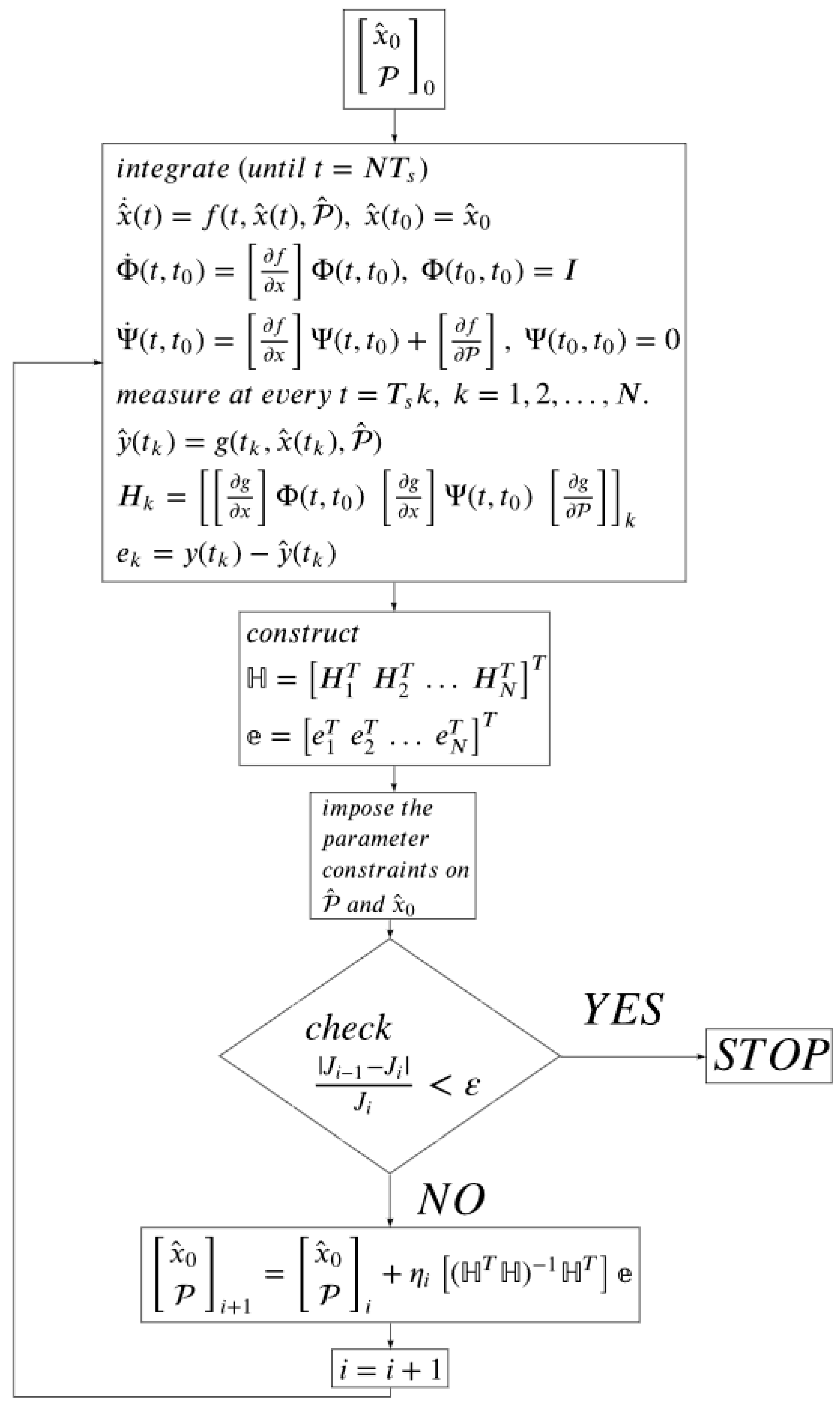
After analytically computing the entries of the matrices $\left[\frac{\partial f}{\partial x}\right],\left[\frac{\partial f}{\partial 𝓅}\right],\left[\frac{\partial g}{\partial x}\right],\left[\frac{\partial g}{\partial 𝓅}\right]$, the GLSDC based parameter estimation algorithm is illustrated in the flowchart diagram given in Figure 1.

4. Simulation Results

To test the effectiveness of the parameter estimation algorithm derived in the previous section, a series of simulations have been conducted. The values of the parameters to be estimated are given in the

Table 1. The numerical values of the parameters used in the simulation.

Parameter	Value	Modified Parameter	Value
$\left(p_1,p_1{}_l,p_1{}_u\right)$	$\left(0.1,0.01,1\right)$	$\left({𝓅}_1,{𝓅}_1{}_l,{𝓅}_1{}_l\right)$	$\left(-1,-100,-0.01\right)$
$\left(p_2,p_2{}_l,p_2{}_u\right)$	$\left(0.1,0.01,1\right)$	$\left({𝓅}_2,{𝓅}_2{}_l,{𝓅}_2{}_l\right)$	$\left(10,0.01,200\right)$
$\left(p_3,p_3{}_l,p_3{}_u\right)$	$\left(1,0.01,2\right)$	$\left({𝓅}_3,{𝓅}_3{}_l,{𝓅}_3{}_l\right)$	$\left(10,1,100\right)$
$\left(p_4,p_4{}_l,p_4{}_u\right)$	$\left(1,0.01,2\right)$	$\left({𝓅}_4,{𝓅}_4{}_l,{𝓅}_4{}_l\right)$	$\left(-1.5,-300,-0.007\right)$
$\left(p_5,p_5{}_l,p_5{}_u\right)$	$\left(1,0.01,2\right)$	$\left({𝓅}_5,{𝓅}_5{}_l,{𝓅}_5{}_l\right)$	$\left(-1,-200,-0.005\right)$

with their corresponding modified versions.

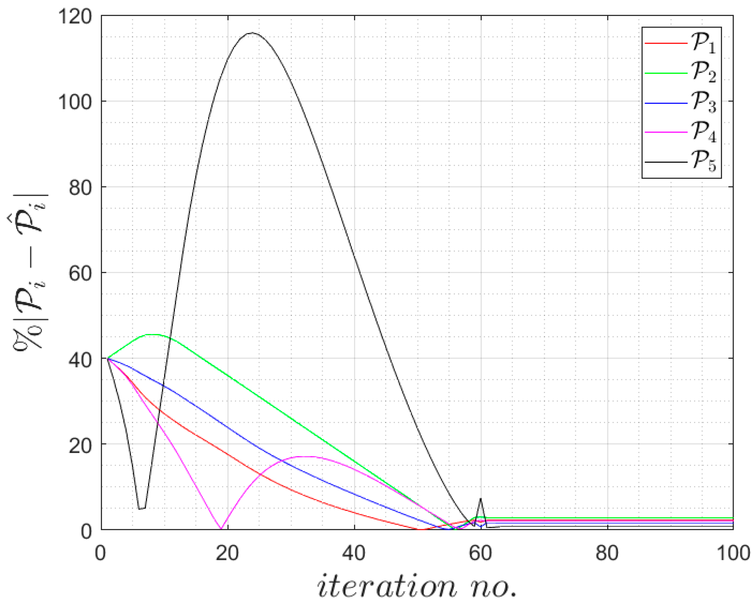
Using the model stated in (1) to (4), the correct output measurement values are collected. The output measurements are assumed to have been corrupted by noise AWGN whose covariance is $0.01I_2$. Using, $T_s=0.01 s$ sampling period, and $3 s$ simulation run time, the collected measurements have been fed to the parameter estimation algorithm. As a result of this, the true values of the parameters have been estimated within less than 5 percent accuracy. The convergence of the parameters is illustrated in the Figure 2. Where, $𝒫$ represents the correct parameter vector, given as ${\left[{𝓅}_1,{𝓅}_2,{𝓅}_3,{𝓅}_4,{𝓅}_5\right]}^T$ and the term. $\widehat{𝒫}$ represents the estimated parameter vector. The subscript $i$ indicates the iteration number in the method.

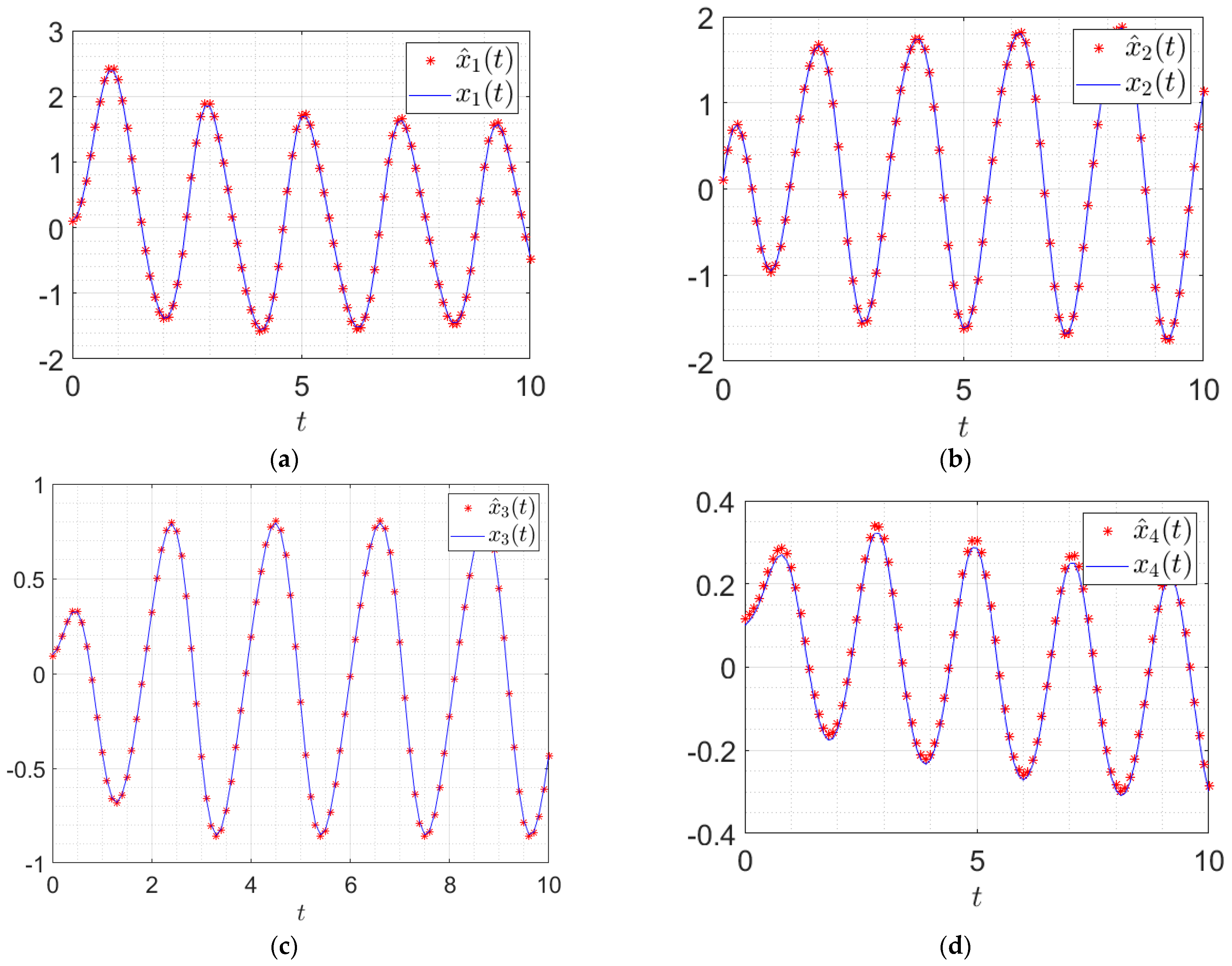
Using those measurement values, the real system parameters are estimated, and the system model is constructed. To assess the performance of the estimation, constructed models’ state trajectories and the state trajectories of the real system are compared. For the same input signal, the state signals of the real and the estimated system is recorded for $10 s$, and given in Figure 3.

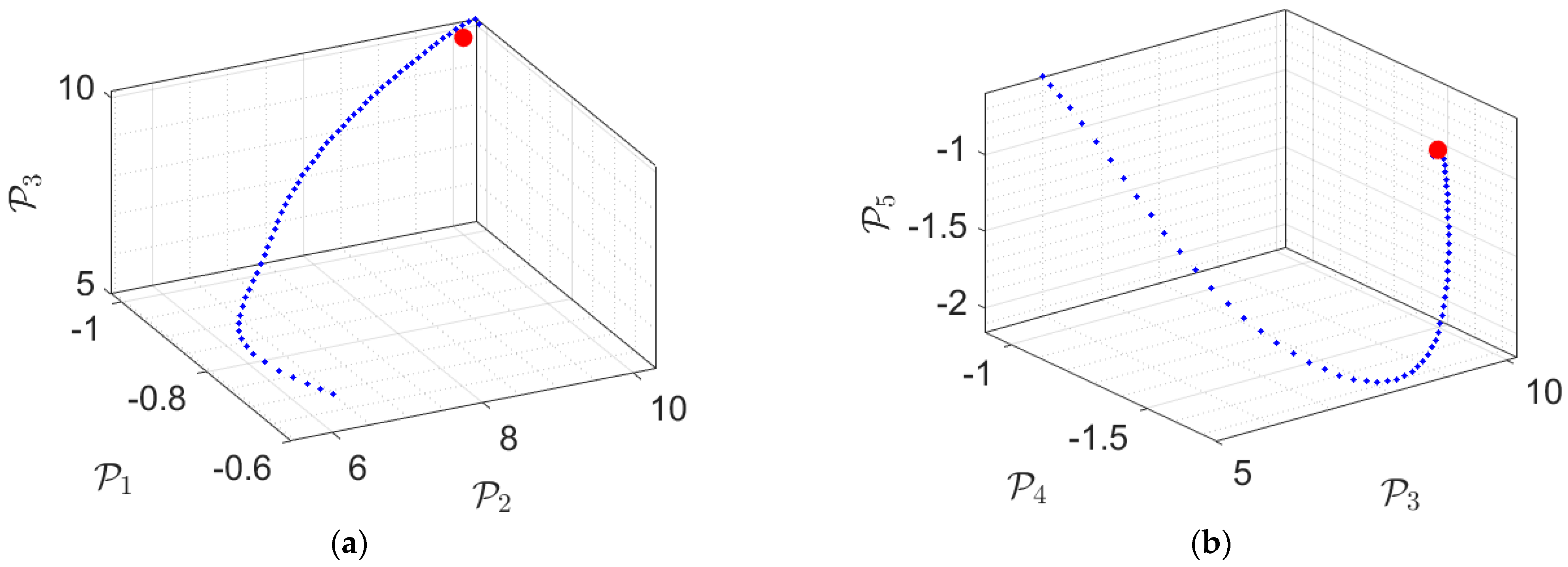
As it can be seen from the trajectories of the states of the real and the model systems, the parameter estimation algorithm is effective in estimating the trajectories of the real system. In addition to the parameters, initial values of the states estimated using the algorithm. The convergence of the estimated terms is given in two separate 3D plots in Figure 4 to illustrate the convergence of the terms.

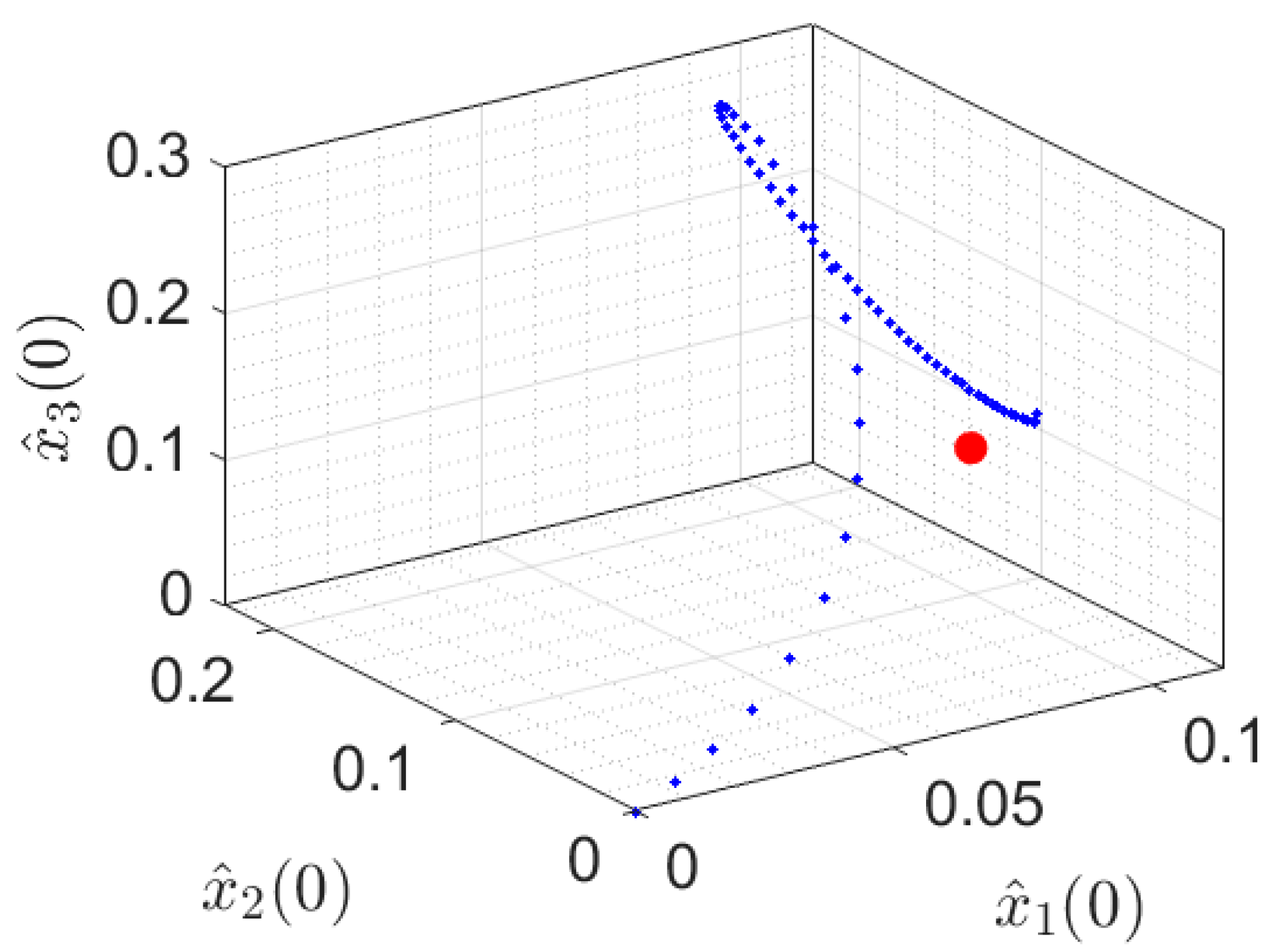
For the illustration of the convergence of the initial values of the states, estimate trajectories are given in Figure 5.

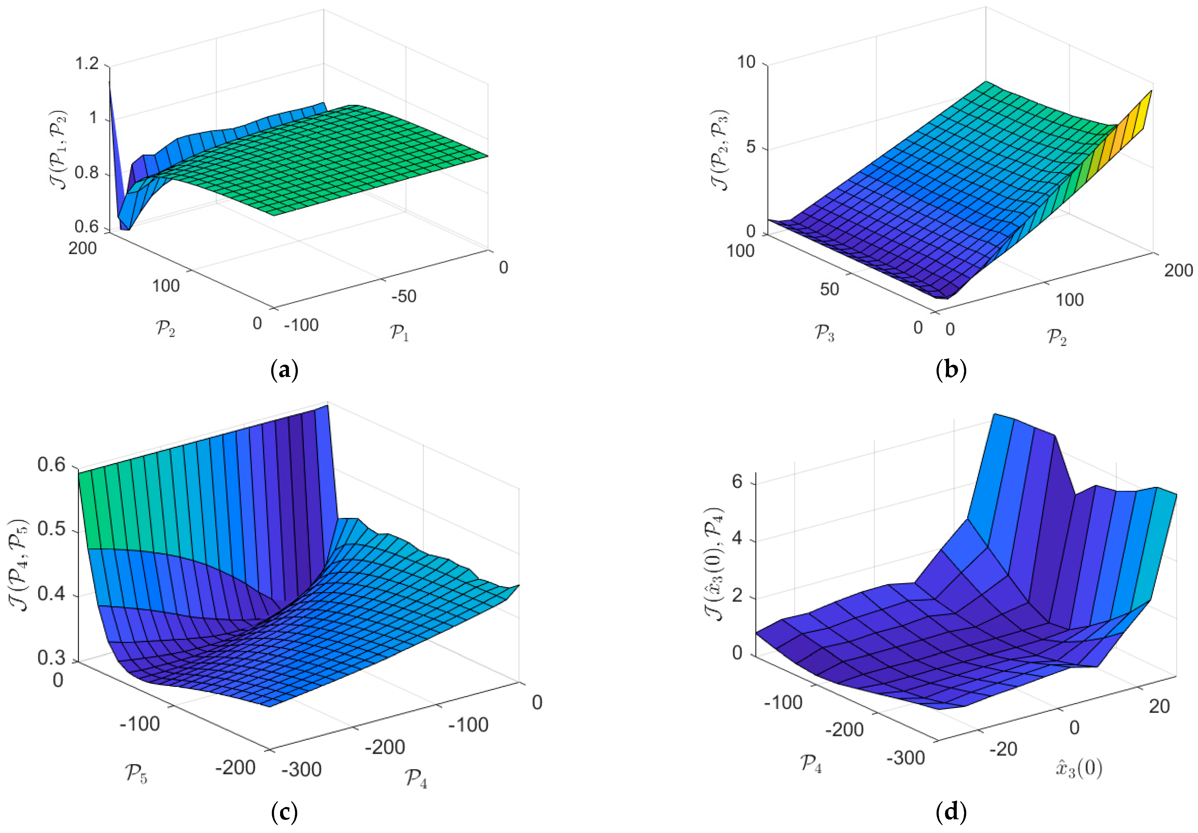
To illustrate the nonconvex nature of the problem, the cost function is plotted against the estimated terms and respective plots are given in Figure 6, where cost with respect to the parameters and initial state values can be analyzed.

For a reasonable starting point, genetic algorithm based methods can be implemented. However, due to the small nature of the problem a couple of initial starting points can be tested in the parameter space and the fittest one can be used.

5. Conclusions

A GLSDC based parameter estimation algorithm is used to obtain a system model for a given PMSM dynamics. GLSDC algorithm is especially useful in estimating the embedded terms in the state space dynamics and an existing assumed dynamic structure for the system. For the cases where there is a possibility to apply a desired signal to the system such that inherent small nonlinearities are made apparent, the effectiveness of the algorithm becomes more evident for the estimating the coefficients of the small nonlinear terms. To prevent a possible numerical error, ${\left({ℍ}^Tℍ+\alpha I\right)}^{-1}{ℍ}^T$ term can be used instead of directly using the pseudoinverse term, ${\left({ℍ}^Tℍ\right)}^{-1}{ℍ}^T$, to update the estimated terms. In addition to that, a moment-based update techniques also can increase the speed of the convergence. The algorithm is tested in a given simulation and the results are given and interpreted accordingly. There are several evolutionary based optimization algorithms can be used to estimate the parameters and the initial state values, however, it has been determined that in general, the number of simulation number that is required to estimate the terms are higher compared with the algorithm that is stated. Additionally, this type of estimation procedure can also be utilized to determine which parameter heavily affect the state trajectory at a given time instant. For example, for some systems, first N data points of the measurement can suffice to estimate a subset of the parameters and last N data points can suffice to estimate the rest of the parameters. Therefore, which parameters affect the state trajectory at the initial time of operation and later time of operation can be analyzed by using that type of algorithm.