1. Introduction
The climate and energy policy of the European Union (EU), including the pursuit of EU climate neutrality by 2050, has a major impact on shaping the national energy strategy [
1,
2,
3,
4]. The regulatory package was adopted in 2009, setting three headline targets for tackling climate change by 2020 (3 × 20% package), in which member states participate according to their possibilities. Poland has adopted the following goals [
5,
6]:
- -
Increasing energy efficiency, by saving primary energy consumption by 13.6 Mtoe in 2010–2020 compared to the forecast of fuel and energy demand in 2007;
- -
Increasing the share of energy from renewable sources in the gross final energy consumption to 15% by 2020;
- -
Contribution to the EU-wide reduction of greenhouse gas emissions by 20% (compared to 1990) by 2020 (in 2005 the levels were: −21% in the EU ETS sectors and −10% in the non-ETS).
In 2014, the European Council kept the trend of counteracting climate change and ratified four targets for 2030 for the entire EU, which, after the changes in 2018 and 2020, are as follows [
6]:
- -
Reduction of greenhouse gas (GHG) emissions by at least 55% compared to 1990 emissions;
- -
At least 32% share of renewable sources in the gross final energy consumption;
- -
Increase in energy efficiency by 32.5%;
- -
Completing the internal EU energy market.
In 2019, the European Commission issued information on the European Green Deal, i.e., the direction of action towards achieving climate neutrality by the EU by 2050. Poland supported this goal, but introduced changes related to the electro-energy transformation and its socio-economic aspects. The result was the approval of the Polish Energy Policy until 2040 in 2021. PEP2040 is one of the nine integrated sector strategies resulting from the Responsible Development Strategy. Additionally, it is also consistent with the National Energy and Climate Plan for 2021–2030 [
6].
In PEP2040, the state and operating conditions of the energy sector were analyzed. The document identifies three pillars on the basis of which eight specific objectives were based, along with an indication of the means for their implementation. One of the long-term directions outlined in the document is the zero-emission energy system, which Poland’s energy transformation is striving for. Reducing the emission level of the electricity sector will be possible through the implementation of low-emission sources, such as nuclear energy, offshore wind energy, or by increasing the role of distributed and civic energy, while ensuring energy security through the ad hoc use of energy technologies based on e.g., gaseous fuels [
6].
The aim of the article is to forecast the consumption of natural gas on the Polish market as an energy raw material ensuring stability of energy supplies during the transformation of the electro-energy system. The transformation process causes that the analyzed time series of raw material consumption are non-stationary and change over time, which results in the rejection of historical statistical data. The article indicates a group of models that can be used to forecast small-number statistical data sets. The theoretical gap that is visible in the analysis of the assumed research problem is the lack of reliable studies indicating mathematical models that can be used to forecast a small number of sets of statistical data. The key element in selecting the theoretical model is the amount of data. There is an ongoing discussion in the literature on the determination of the size of the input data set for modeling [
7,
8,
9,
10]. It is indisputable that the predictive model depends on the number of inputs. What is new, however, is the trend that suggests the use of artificial neural networks (ANN) as techniques dedicated to the analysis of small data sets. The article analyzes the mathematical models used to forecast natural gas consumption and proposes ARIMA class models and LSTM artificial neural networks.
The structure of the document is as follows:
Section 2 describes gaseous energy minerals in Poland, while
Section 3 is devoted to the analysis of gas trade.
Section 4 is a literature review of the models used to forecast natural gas consumption.
Section 5 describes the model of natural gas consumption on the Polish market.
Section 6 provides the results and discussion, and
Section 7 presents a summary of the work.
2. Gas Energy Minerals in Poland
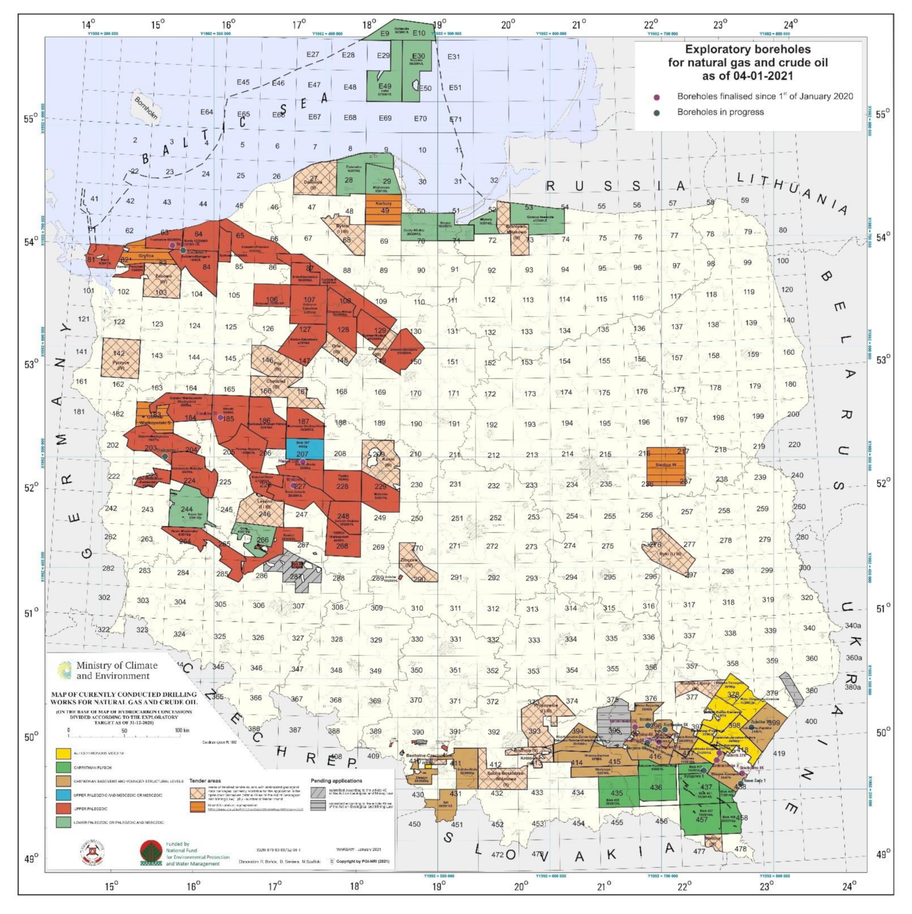
The main region of occurrence of natural gas deposits in Poland is the Polish Lowlands, the Carpathian foothills. Low gas resources are found in the deposits of the Carpathian area and in the national economic zone of the Baltic Sea, as shown in
Figure 1.
In the Polish Lowlands, natural gas deposits occur in the Fore-Sudetic and Greater Poland regions in the Permian formations, and in Western Pomerania in the Carboniferous and Permian formations. The gas occurs in the bulk and block-type deposits with water or gas-pressure conditions of exploitation [
12]. There are only a few deposits in this area that contain high-methane gas, while the remaining deposits are dominated by nitrogen-rich gas (methane content between 30% and 80%). Deposits in which natural gas contains over 90% nitrogen are also found in the Polish Lowlands (the Cychry and Sulęcin deposits in the Zechstein Dolomite).
In the foothills of the Carpathians, natural gas deposits occur in Jurassic, Cretaceous and Miocene deposits. It is usually high-methane, low-nitrogen gas. The deposits are structural and lithological, multi-layered, less often massive, producing under gas-pressure conditions.
In the Carpathians, natural gas occurs in Cretaceous and Palaeogene formations, both in standalone deposits and accompanying oil or condensate deposits [
12]. The gas is high in methane. The methane content is above 85%.
In the Polish economic zone of the Baltic Sea, natural gas occurs independently in the B4, B6, B21 fields and together with crude oil in the B3 and B8 fields.
Table 1 summarizes the amount of recoverable natural gas resources from gas fields, as well as oil and condensate fields, considering the degree of their recognition and the state of development.
The documented deposits of the Polish Lowlands currently contain 73.4% of recoverable natural gas resources. A total of 21.9% of these resources are located in the foothills of the Carpathians. The resources of the Baltic and Carpathian Sea zones play a minor role (3.6% and 1.1% of national resources, respectively). In 2020, the state of recoverable natural gas resources amounted to 143.92 billion m3 (in total, on-balance and off-balance sheet resources) and the resources decreased by 0.33 billion m3 compared to the previous year. In 2020, the Gnojnica field was included in the balance sheet (documented recoverable balance resources: 148.59 million m3). The largest increases in resources were recorded in the Brońsko field (new wells were put into operation, mining intensification treatments) and in the Trzebusz (geological and investment documentation approval), Paproć, Załęcze fields (mainly better exploration of the deposit by exploitation and activities intensifying production). Resource losses were mainly caused by mining. The recoverable resources of the developed natural gas deposits amount to 95.81 billion m3, which constitutes 66.6% of the total amount of recoverable resources. The industrial resources of natural gas in 2020 amounted to 73.51 billion m3. From domestic raw materials, Poland covers only 20% of the demand.
3. Natural Gas Trading
The natural gas market differs from the markets of other commodities due to operational and logistic conditions. In the case of trading in natural gas, its transport plays a very important issue. The market trade of gas takes place with the use of gas pipeline systems. In addition, sometimes geographic location also determines the issue of suppliers and recipients [
13]. Gas is a raw material, the transport of which requires large investment outlays in the long term (e.g., construction of gas pipelines), and the infrastructure built for gas transport is used only for this purpose (there are no such restrictions in the transport of other goods, including steam coal or oil). It also means that suppliers and customers are bound by long-term contracts due to the enormous costs of building infrastructure. Diversification of supplies and prices to some extent is possible thanks to the construction of LNG regasification terminals for receiving liquefied natural gas. However, here too there are many problems related to, for example, the parameters and properties of the gas. As natural gas is supplied via gas pipelines or special tankers (so-called methane carriers), three main gas trade markets can be distinguished, which (due to the possibility of supply) are partially hermetic. The first market is North America and the second is Europe. Sometimes both markets are referred to as the Atlantic market (similar to coal trading). The third market, on the other hand, is the Southeast Asia region, also known as the Pacific market.
Due to the specificity of the gas market resulting from the possibility of its transport, there is no single global gas market. This means that for each of the three local markets (American, European, and Asian) a different price level is set, with the European and Asian markets being dominated by prices set in long-term contracts. Long-term contracts prevail on the European market due to the fact that most of the gas is supplied via gas pipelines from Russia, Norway, the Netherlands and Algeria. As the main supplier of gas to the European market is Gazprom (Saint Petersburg, Russia), approximately 3/4 of the supplies are made through fixed contracts, concluded separately in the case of Gazprom with each of the countries. Gas prices in such contracts are tied to the prices of crude oil and its products but follow oil price movements with a lag of 1–3 quarters [
14]. Often, the price of Russian natural gas delivered to the German border is used as a reference price for price comparisons on the European gas market.
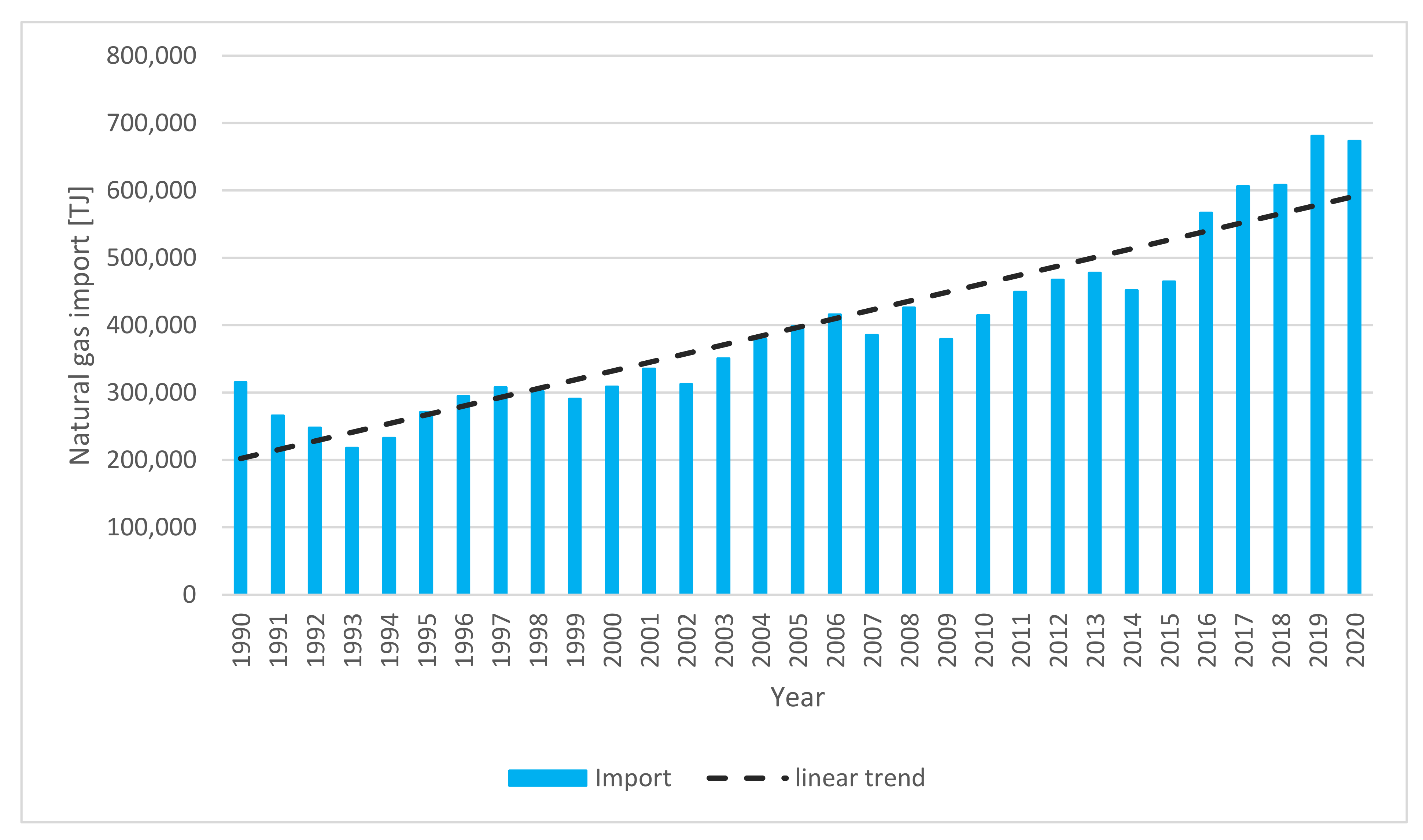
To meet the demand for natural gas in Poland, it is necessary to import the raw material—mainly from Russia, Germany, Norway, the Czech Republic, Ukraine and the countries of Central Asia. Natural gas imports have a growing tendency. Over the period 1990–2018, imports increased on average by 7%, as shown in
Figure 2.
The Polish natural gas market is becoming a competitive one [
16]. Since 2013, sales through the stock exchange have been in force, initially it was 30% of the market volume, and from 2015, 55%. The stock exchange tools developed in stages and the aforementioned exchange obligation are the basis for the creation of a liquid, wholesale natural gas market in Poland, and in the future, it will allow the recipient to change the supplier [
6].
4. Literature Review of Forecasting Natural Gas Consumption
In the literature on the subject, it can be stated that the forecasting of natural gas consumption was studied in several different planes, the consumption on the global and domestic market, in the commercial and residential sectors as well as at the level of individual consumers, as well as the gas distribution system was analyzed. Various data, such as economic parameters, weather data, historical gas consumption, or information on historical energy consumption or household survey data, were used for the research.
The Hubbert curve model was used as the first forecasting tool for natural gas consumption. In his works, Hubbert [
17,
18] analyzed the production of fossil fuels and after analyzing the time series of the production curves, he noticed that these curves are similar, and the time series have similar properties. Statistical models related to natural gas consumption were developed in the 1960s and have been widely used as forecasting tools ever since. In [
19], Balestra and Nerlove used statistical tools to analyze time series in forecasting natural gas demand. The demand for electricity and natural gas in the northeastern United States was predicted by regression analysis in Beierlein et al. [
20]. Piggott [
21] applied the Box–Jenkins modeling. Herbert et al. [
22] also used regression analysis, while the linear regression equation and residual study were used in Herbert [
23]. ARIMA models are described in Liu and Lin [
24] and Oylum and Akgün [
25]. Liu and Lin [
24] used the linear LTF method and the CCF (cross-correlation function) method. Brabec et al. [
26] used the non-linear model ARIMAX and ARX. Lee and Singh [
27] built a model using the multiple regression technique, exactly the generalized Tobit model. In 1988, Werbos in [
28] used back-propagating artificial neural networks to forecast the cold gas market and found that trained back-propagating ANNs outperform traditional statistical methods such as regression. Then, del Real A.J., Dorado F., Durán J. in [
29] proposed the use of deep learning techniques to forecast energy demand. They presented a mixed architecture consisting of a convolutional neural network (CNN) coupled to an artificial neural network (ANN). Khotanzad et al. [
30] Brown et al. [
31] and Brown and Iftekhar [
32] developed and used models based on artificial neural networks with feedforward to predict gas consumption and compared them with a linear regression model. Suykens et al. [
33] and built a model of gas consumption in Belgium using non-linear artificial neural networks.
There are no studies in the literature related to forecasting natural gas consumption with the use of LSTM (Long Short-Term Memory) networks, the architecture of which is also recursive, but unlike standard recursive networks, the LSTM network has a feedback loop, thanks to which it can process not only single points data, but also entire sequences. Hence, these networks are used to classify, process and forecast based on time series data, especially where there are delays of unknown duration between important events. LSTMs were developed also to solve the vanishing gradient problem encountered in training traditional recursive networks (RNNs). It should be noted that in RNN networks, learning consists in copying the same networks, each of which transmits a message to the successor, while in networks with feedback, the output layer of the network has an impact on the input layer. LSTMs are a special type of RNN capable of learning long-term relationships. They were introduced by Hochreiter and Schmidhuber in 1997 [
34], and then refined and popularized in subsequent works [
35,
36,
37,
38]. They work extremely well with long-term dependency problems.
5. Materials and Methods
Data from the IEA [
15] and BP [
39] for the period from 1968 to 2020 were used to forecast the demand for natural gas. The study took into account both linear models, i.e., models in which the forecast can be presented as a linear combination of previous series and residuals of the model as well as nonlinear models. The first group was represented by ARIMA models. These models are the canon of statistical time series models [
40]. The second group of non-linear models was represented by artificial neural networks. In the literature on the subject, one can find many arguments that the time series of economic variables (macroeconomic and financial) behave in a non-linear manner. For example, in the article [
41] the authors mention such empirical time series properties as: their different behavior in periods of growth and recession or in periods of low and high volatility. Akbal and Demirberk Ünlü proposed the use of hybrid deep learning methods [
42]. According to the results of the analysis, it is shown that the most important predictor used which consists of feed-forward neural networks, convolution neural network and long short-term neural networks
ARIMA models owe their popularity to Box and Jenkins, who in 1970 published the book Time Series Analysis: Forecasting and Control, in which they systematized the current state of knowledge related to time series modeling. They also proposed a three-step procedure, thanks to which it was possible to identify, estimate and verify ARIMA models. ARIMA models are treated as linear models, and linearity refers to the construction of the model in which the modeled yt value is a linear combination of past implementations and past and current random disturbances εt.
The form of the ARIMA model (
p,
d,
q) for the time series can be presented as follows [
43]:
where
εt is a white noise process with mean 0 and variance σ
2,
B is the backward shift operator, and φ(
z),
θ(
z) are polynomials of degrees
p and
q, respectively. To ensure the reversibility and casualty of the process, it is required that both polynomials do not have roots outside the unit circle. The problem of identifying the ARIMA model consists in indicating the value of autoregressive delays
p, the order of integration d and the number of delays of the moving average
q. If the degree of integration of the process
d is known, the choice of the order
p and
q consists in comparing the values of a given information criterion for models built for various combinations of
p and
q. If the degree of integration is unknown, then the informative criteria cannot be used as for different
d values their values are not comparable [
44].
In the case of artificial neural networks built for the purposes of time series forecasting, the role of explanatory (input) variables is played by delayed series values. Such a structure of the network causes that it becomes a non-linear equivalent of the autoregressive model. Considering the prognostic function of the model being built, the proposed network should be relatively simple (models that are too detailed, over-adjusted to the data have poor generalization properties). Therefore, the LSTM (Long Short-Term Memory) network was used in the study. The LSTM neural network architecture is recursive and is used in deep learning methods. Unlike standard recursive networks, the LSTM network has feedback, so it can process not only individual data points, but entire sequences as well. Hence, these networks are used to classify, process and forecast based on time series data, especially where there are delays of unknown duration between important events. The LSTM network computes the mapping from the input sequence
x = (
x1, …,
xt) to the output sequence
y = (
y1, …,
yt) by computing the network unit activation using the following iteration equations from
t = 1 to T [
34]:
where conditions
W,
U are weight matrices, conditions
b denote the polarization vectors (
bi is the input gate polarization vector),
σ is the activation function,
I,
f, o and
c are respectively input gates, forgotten gates, output gates and activation vectors of cells, of which all are the same size as the activation vector of the output cell, i.e., the result of the vectors, and
g and
h are functions of the input and output activation of the cell.
Proper selection of parameters causes that the constructed network corresponds to specific forms of ARIMA models, for which there are no restrictions on parameters.
The accuracy of forecasts was assessed using forecast assessment measures:
- -
Mean error of ex post forecasts (mean error,
ME), [
43]:
The mean forecast error informs about the average deviation of the forecast values from the actual realizations of the forecast variable (i.e., the load). If the ME value is positive, then the forecasts are on average too low (underestimated), while when the ME indicator value is negative, then the forecasts are on average too high (overestimated).
- -
Mean absolute error of ex post forecasts (mean absolute error,
MAE), [
43]:
- -
Root mean square error,
RMSE, [
43]:
The root of the mean square error informs about how far, on average, the actual realizations of the forecast variable deviate from the calculated forecasts. A significant difference between the mean absolute error MAE and the root mean square error RMSE means the occurrence of errors with very different (large and small) values during the verification period of forecasts.
- -
Mean square error,
MSE, [
43]
The mean percentage error informs what percentage of the actual implementations of the forecast variable are forecast errors during the period of their verification.
6. Results and Discussion
The ARIMA models and the LSTM artificial neural networks were used to forecast the volume of natural gas consumption, which were used to forecast the residuals obtained from the ARIMA model (1,1,0). Additionally, in addition to historical consumption, the mathematical model also includes a forecast of prices of primary fuels, i.e., crude oil, natural gas and thermal coal, in imports to the European Union. The work uses the forecasts developed by the European Commission in the report EU energy, transport and GHG emissions trends to 2050 reference scenario 2013 [
45]. This document is based on European energy, and transport trends to 2030 from 2009 [
46].
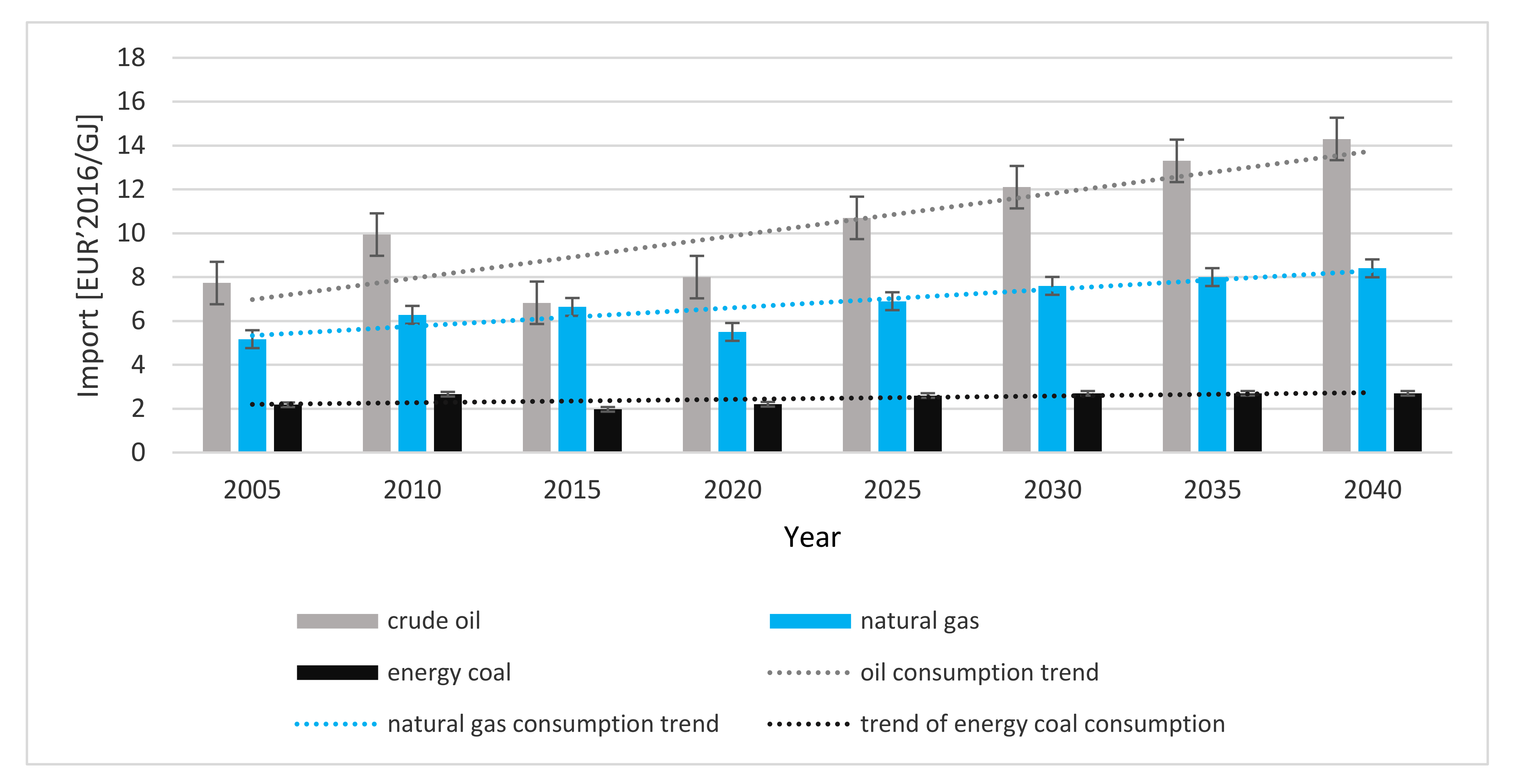
In
Figure 3, the forecasts indicate an increase in the prices of all raw materials. After 2012, world prices of fossil fuels changed significantly. This is mainly due to the reserves of shale gas and other unconventional hydrocarbons. Prices are expected to follow new, rather different trajectories, especially for gas. The models implemented large adjustments to the availability of conventional gas and oil resources (according to the USGS, IEA), and included global estimates of unconventional gas resources (tight sands, shale gas and seam methane) based on IEA estimates. The change means that the natural gas resource base increases more than 2.5 times, which has a significant impact on prices. In terms of economic factors, higher GDP growth is also projected, particularly in China, India, and the Middle East and North African regions.
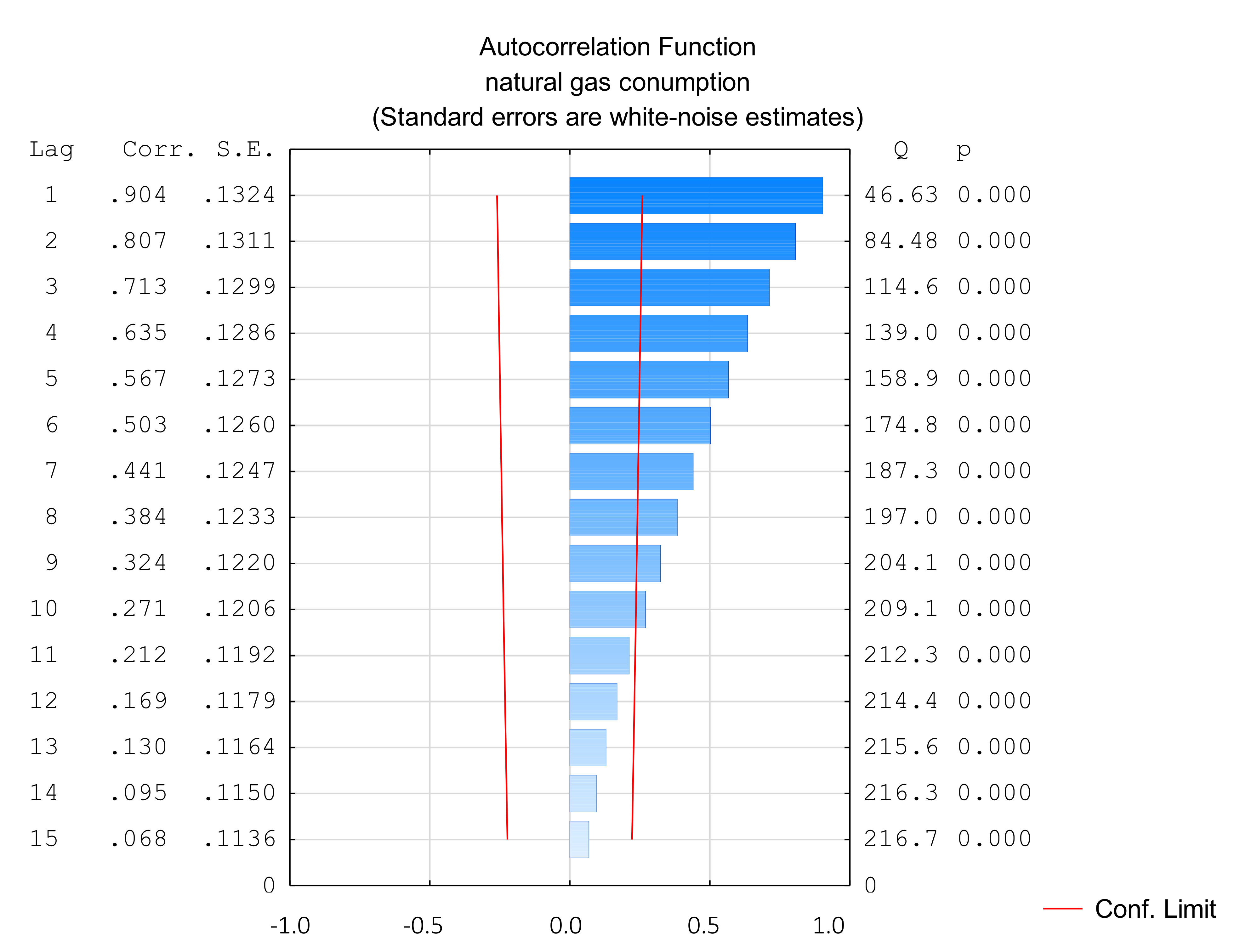
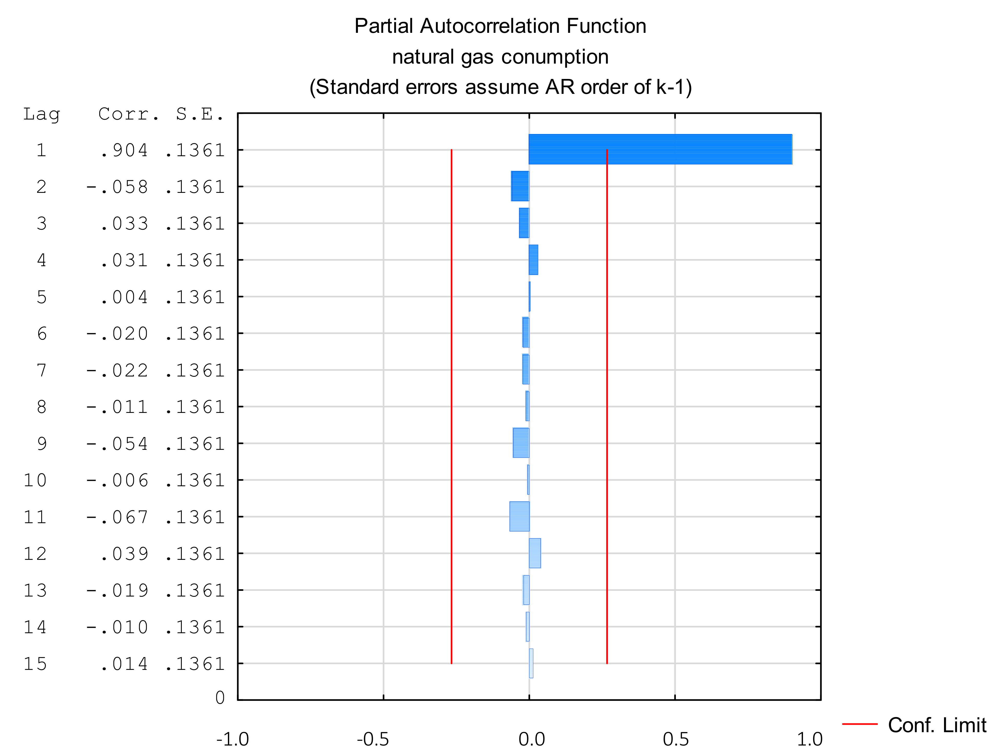
The basis for the identification of the autoregressive model is the empirical autocorrelation function and the empirical partial autocorrelation function.
Figure 4 and
Figure 5 show the values of these functions for the delays
p = 1, 2, … 15.
Based on the graph presented in
Figure 4, it can be concluded that the empirical autocorrelation function decays exponentially, while the graph presented in
Figure 5 shows that only the partial autocorrelation for d = 1 is significantly different from zero.
The ARIMA model introduced by Box and Jenkins contains both autoregressive and moving average parameters and introduces the differentiation operator into the model, which is to ensure the stationarity of the process (mean constant in time, variance, and autocorrelation). To determine the necessary level of differentiation, the data plot and the autocorrelogram should be analyzed. In the case of natural gas consumption, there are significant changes in the level (strong increase and decrease), which requires first-order differentiation (lag = 1). Stationarity analysis was performed using Augmented Dickey Fuller test (ADF). The ADF is a standardized unit root test for determining the effect of trends on data, and its results are analyzed by the probability of the test [
35].
The following hypotheses were assumed:
Hypothesis (H0). There is no unit root for p < = 5%.
Hypothesis (H1). There is unit root for p > 5%.
The p-values equal 34%, which means that the process is non-stationary, and this is the result of the transformation of the energy market in Poland. In the years 1965–1985, gas consumption increased. Then there is a sudden drop, by about 19% until 1992. Since 1993, there has been a gradual increase in demand by about 7% per year. As a result of an in-depth analysis of stationarity, the historical data from the period 1965–1992 was re-jected, as they are not related to the current and future gas consumption. This, in turn, allowed for the process to be stationary (p-values 4.6%) but the reduction of the input data set, the forecasting process will be performed on a small set of input data.
There is a trend in the literature on predicting small sets of data suggesting the use of artificial neural networks (ANN) as reliable techniques, in which their performance is independent of the total number of input data (7–10).
Based on these studies it has been proposed to build a hybrid ARIMA model (1,1,0) and LSTM artificial neural networks, which were used to forecast the obtained residuals from the ARIMA model (the residual autocorrelation was checked using the Breusch–Godfrey test). The following predictors were used in the model: historical consumption of natural gas, prices of primary fuels, i.e., crude oil, natural gas and thermal coal, in imports to the European Union.
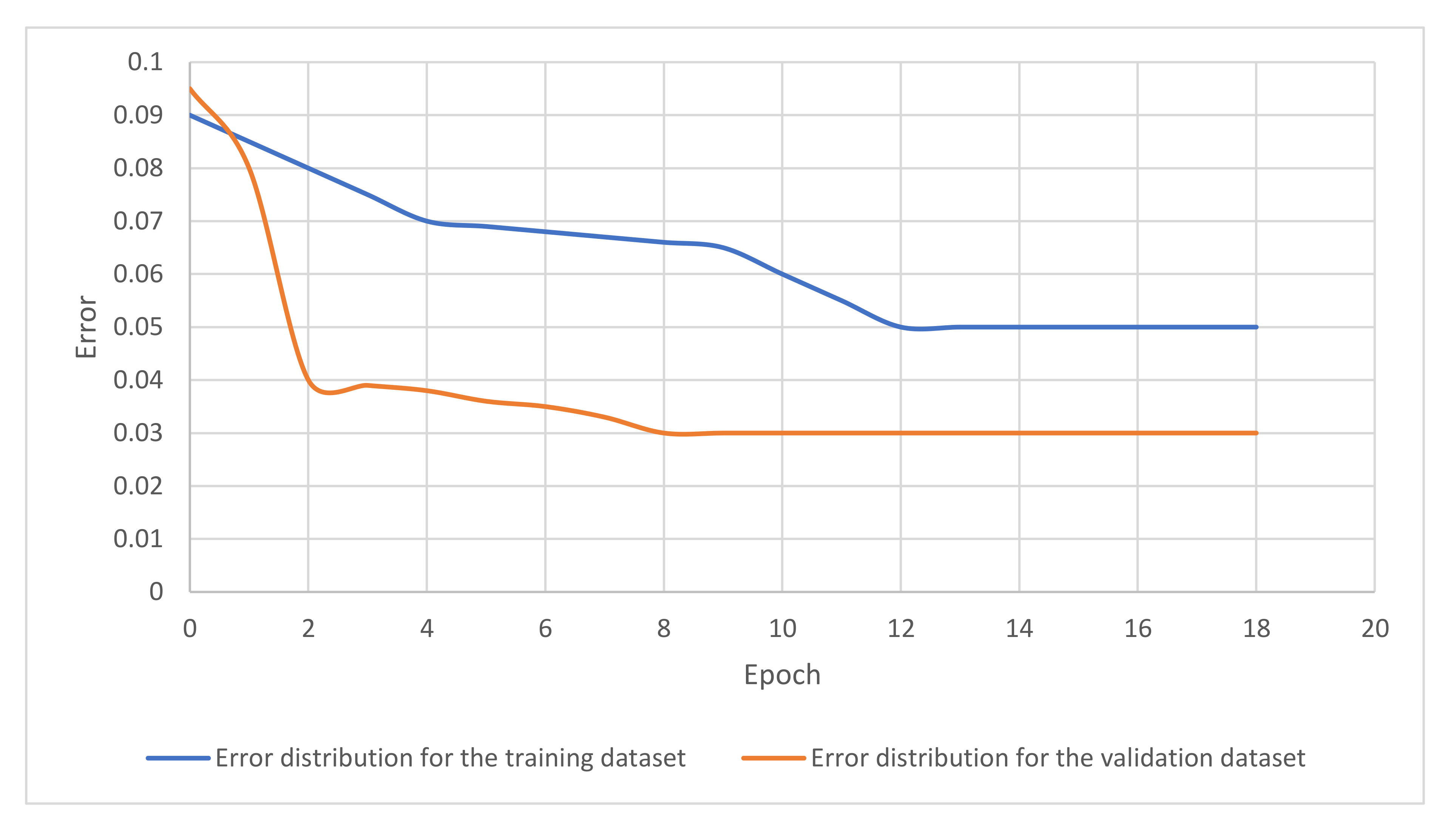
The obtained residues were introduced into the LSTM artificial neural network in the TensorFlow environment. The model was trained on 21 data using cross entropy, Adam’s optimization and 18 epochs. Twenty percent of the data was used for model validation. The model is designed from the input (LSTM), the hidden (dropout) to the output (dense layer). The residuals from the model were introduced to the input layer. The output layer is the prediction.
Figure 6 presents the distribution of network learning errors.
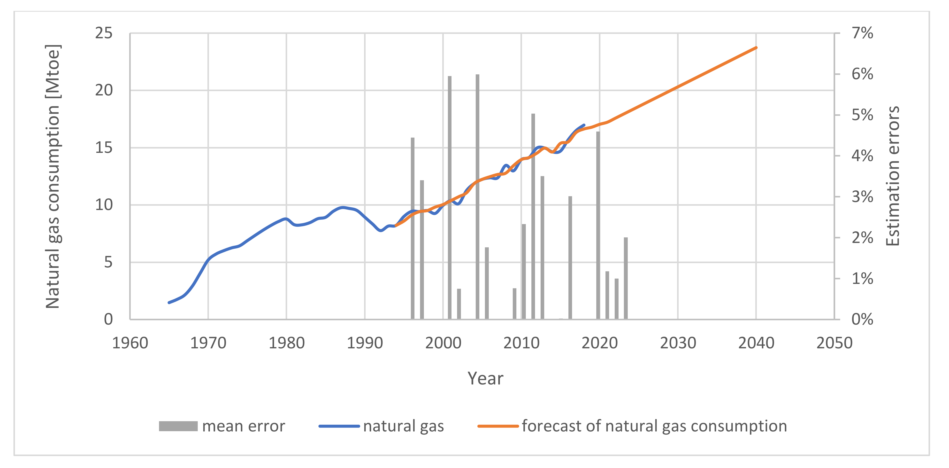
After training on the test data set, you can see that the model achieves 98% accuracy for the validation data. The comparison of theoretical and real values and the error distribution are shown in
Figure 7.
The set of statistical data used for forecasting was reduced to the period 1993–2020 due to the change in the natural gas consumption process in Poland. As a result of the analysis of volatility measures, it can be observed that there has been a decrease in the consumption of natural gas by about 19%. After 1993, there was a gradual increase in demand by about 7%. A hybrid ARIMA model (1,1,0) and LSTM artificial neural networks were built for consumption forecasting. The following predictors were used in the model: historical consumption of natural gas, prices of primary fuels, i.e., crude oil, natural gas and thermal coal, in imports to the European Union. The validity of the constructed model was assessed using the tools described in the “Materials and Methods” section. The average forecast error is −0.00032 Mtoe, which means that the forecasts are on average too high (overestimated). The mean absolute error of ex post forecasts is 0.219922 Mtoe, while the root of the mean square error is 0.321005 Mtoe. The difference between the errors is at the level of 30%, which proves a significant variation in values. The average percentage error is 2%, which means that the model largely models the real gas consumption course.
7. Conclusions
The analyzes carried out in this paper concerned issues related to the natural gas market in Poland. It has been shown that during the transformation of the energy–electric system, Poland intends to ensure the stability of energy supplies using natural gas. Unfortunately, Poland covers only 1/5 of the demand for the raw material from its domestic deposits. The rest must be imported from Russia, Germany, Norway, the Czech Republic, Ukraine and Central Asia. Despite the fact that none of the analyzes in the article referred directly to the problems related to energy security in the European Union, some of the results obtained can be considered precisely in the context of security. The results of analyzes that can be related to this issue concern long-term relations between the prices of energy resources on the European market. The results of the analysis clearly showed that, in the analyzed period, there was a long-term equilibrium between the prices of coal, oil and gas on the European market, and thus the market for the main prices of primary fuels in Europe was integrated. The leading price, which shaped the remaining energy commodity prices in the long run, was the price of crude oil, and the prices of Russian natural gas and thermal coal in ARA ports were imitative. This means that in the long term, the diversification of energy sources (the three basic energy raw materials) aimed at ensuring energy security in the European Union may be endangered. The results also suggest that one of the possibilities of hedging against changes in energy commodity prices may be an increase in the share of renewable energy sources in energy consumption in the European Union. The second area of analysis was to build an effective model for forecasting natural gas consumption. This issue is extremely important because, as previously shown, natural gas is to ensure the stability of energy supplies for Poland during the energy transformation period. As part of the study, a model was built based on a combination of deep learning methods with statistical methods. The ARIMA model (1,1,0) and LSTM artificial neural networks were proposed. The accuracy of the modeling results was verified by error analysis and model validation ratios. This model is characterized by a high adjustment to real data. Using artificial LSTM neural networks to analyze the residuals obtained from the ARIMA model (1,1,0) in the years 1993–2020, a good adjustment to the time series of natural gas consumption is obtained and good forecasts up to 2040. Description of the phenomenon and forecast using artificial neural networks are much better than those based on the analysis of the same trend, seasonal and cyclical fluctuations. However, further research is needed to investigate the fit of a model that considers the effect of significant variables in the socio-economic environment on gas consumption.


