On Thermal Energy Transport Complications in Chemically Reactive Liquidized Flow Fields Manifested with Thermal Slip Arrangements

Abstract

Heat transfer systems for chemical processes must be designed to be as efficient as possible. As heat transfer is such an energy-intensive stage in many chemical processes, failing to focus on efficiency can push up costs unnecessarily. Many problems involving heat transfer in the presence of a chemically reactive species in the domain of the physical sciences are still unsolved because of their complex mathematical formulations. The same is the case for heat transfer in chemically reactive magnetized Tangent hyperbolic liquids equipped above the permeable domain. Therefore, in this work, a classical remedy for such types of problems is offered by performing Lie symmetry analysis. In particular, non-Newtonian Tangent hyperbolic fluid is considered in three different physical frames, namely, (i) chemically reactive and non-reactive fluids, (ii) magnetized and non-magnetized fluids, and (iii) porous and non-porous media. Heat generation, heat absorption, velocity, and temperature slips are further considered to strengthen the problem statement. A mathematical model is constructed for the flow regime, and by using Lie symmetry analysis, an invariant group of transformations is constructed. The order of flow equations is dropped down by symmetry transformations and later solved by a shooting algorithm. Interesting physical quantities on porous surfaces are critically debated. It is believed that the problem analysis carried out in this work will help researchers to extend such ideas to other unsolved problems in the field of heat-transfer fluid science.

1. Introduction

The study of heat transfer in fluids has a wide range of applications in various disciplines, such as stream generators, die temperature control, concrete heating, distillation, extrusion, hot mix paving, printing and laminating, to name only a few. It is very expensive to perform individual experiments on heat transfer in fluids and extract useful information. Therefore, investigators always prefer to carry out computational analysis and then carry out particular experiment to obtain maximum benefits. Owing to such thought, researchers from several fields, namely, biology, meteorology, geophysics, astrophysics, oceanography, civil engineering, mechanical engineering, biomedical engineering and chemical engineering, have prioritized the computational analysis of both Newtonian and non-Newtonian fluid flows by means of heating surfaces in different configurations with heat transfer aspects—such as Sarma and Rao [1], who investigated an incompressible viscoelastic fluid over a semi-infinite stretching sheet in the presence of power-law surface heat flux/temperature, taking into account the impacts of viscous dissipation as well as internal heat generation or absorption. The skin friction coefficient and heat transmission, among other important physical parameters, were observed; for large Prandtl numbers, asymptotic findings for the temperature function were reported. Chamkha and Issa [2] investigated the influences of dual convection currents on the time-dependent flow of an electrically conducting heated fluid across a stretched vertical surface. To accommodate for probable fluid wall suction or injection, the surface was assumed to be permeable, maintained at a changeable temperature, and to have a linear velocity. Flow equations were developed using the Boussinesq approximation and boundary-layer theory. The converted equations were numerically solved using the finite-difference method after an appropriate transformation. Comparisons were made with previously published studies, and the results were found to be very similar. Full parametric research was carried out, with a sample set of graphical data for temperature, velocity and the time evolution of the skin-friction and wall heat transfer coefficients reported and discussed. Andersson et al. [3] investigated heat transfer aspects in a laminar liquid layer on a horizontal stretched sheet. An accurate transformation was used to reduce the flow equations to ordinary differential equations. Regarding the selective values of the Prandtl numbers, and the unsteadiness parameter, they solved the two-parameter problem numerically. It was observed that the temperature increased monotonically from the elastic sheet to the free surface. Hou and Lin [4] used activation energy asymptotics to investigate heat transfer aspects in the extinction of dilute spray flame flows. Flame propagation modes that are totally vaporized and partially vaporized have been identified. Internal heat transfer, which is influenced by liquid fuel loading and the spray’s initial droplet size, results in heat gain and loss for rich and lean sprays, respectively. The burn intensity of the lean methanol-spray flame and the rich methanol-spray flame was found to be reduced and enhanced by combining flow stretch and the Lewis number. The flow and heat transport of a viscoelastic fluid over a non-isothermal stretching sheet was investigated by Abel et al. [5]. The viscosity of the fluid was anticipated to change with temperature. The existence of a fluid with a changing viscosity causes non-linearity in the boundary value. The coupled non-linear boundary value issue was solved using a numerical shooting approach for two uncertain beginning conditions and a fourth-order Runge–Kutta integration strategy. The effect of the fluid permeability parameter, viscosity, and the visco-elastic parameter in various scenarios was investigated for two separate cases. The key conclusion of their research was that when the flow was through porous media, the effect of fluid viscosity reduced the wall temperature profile dramatically. Furthermore, the permeability parameter had the effect of lowering skin friction on the sheet. Finite element outcomes were reported by Bhargava et al. [6] for micropolar fluids with a mixed convection effect. The results of numerically solving the governing partial differential equations using the finite element approach were compared to those obtained using the quasi-linearization scheme. The impact of surface conditions on velocity and temperature functions has been investigated. Micropolar fluids have been discovered to aid in the lowering of drag forces while simultaneously acting as a cooling agent. Zakaria [7] investigated heat transmission from a non-isothermal stretched sheet. The governing equations for momentum and energy were solved using the successive approximation approach. Regarding velocity and temperature, the impacts of the coefficient of the elastic fluid velocity, Alfven velocity, relaxation time parameter and Prandtl number were discussed. For the subject under consideration, numerical results were provided and graphically illustrated. Khan and Sanjayanand [8] examined the flow and heat transmission of a viscoelastic boundary layer over an exponentially stretched continuous sheet. The highly nonlinear momentum equation had an approximate analytical similarity solution, and the heat transfer equation had a confluent hypergeometric similarity solution. Numerical solutions produced using the Runge–Kutta shooting method were used to validate the solution for the stream function. The flow directional coordinate was exponentially dependent on heat flux, temperature, and velocity. The impacts of several physical factors on the flow field were discussed. The mass and heat fluxes for fluid flow by means of the exponentially stretched surface were examined by Sanjayanand and Khan [9]. In this work, the impacts of elastic deformation and viscous dissipation were considered. The extremely non-linear stream function problem had a zero-order analytical local comparable solution, and the prescribed boundary concentration flux was exponentially related to the flow directional coordinate in these solutions. The impact of elastic deformation on heat aspects was investigated. Salem [10] investigated a heated viscoelastic fluid across a continually stretched surface with a magnetic field effect. The thermal conductivity and viscosity of the fluid were supposed to change with temperature. The fundamental equations were numerically solved to examine the impact of flow variables. Relevant developments in fluid flow fields in various frames can be found in Refs. [11,12,13,14,15,16,17,18,19,20,21,22,23,24,25,26,27,28,29,30,31,32,33,34].

We observed that heat transfer in Tangent hyperbolic fluid flow subject to a porous surface in the presence of chemically reactive species has not been examined on a wide scale due to the acquisition of a coupled non-linear differential model. Therefore, the strength of this article is its numerical findings on non-Newtonian fluid flow in three different physical situations. To support this idea, the draft was designed into five various sections. The motivational background literature is reported in Section 1. The mathematical formulation for thermally magnetized Tangent hyperbolic flow fields, along with heat generation, heat absorption, chemically reactive species, and porous medium is detailed in Section 2. The problem is translated mathematically and the concerned flow equations are firstly reduced using symmetry analysis and then solved numerically by means of the shooting method. The adopted numerical methodology is reported in Section 3. The impacts of flow regulatory variables are debated in Section 4, with the corresponding tables, line graphs, and streamlined patterns. The obtained outcomes are also validated by carrying out comparisons with the existing literature as well. The conclusions of the present attempt are given in Section 5. We believe that the present findings will help readers to gain important information on utilizing Lie symmetry analysis in unsolved fluid flow problems and on the mechanics of non-Newtonian fluid flows over porous thermally magnetized stretched surfaces.

2. Mathematical Formulation

Accurate flow formulation is an important part of computational fluid dynamics analysis. For the present physical design, we considered non-Newtonian fluid flow over a porous surface. The aforementioned flow field interacts with an external magnetic field. The novelty of this is enhanced by considering the energy equation, along with heat absorption and heat generation effects. The concentration equation is also considered, with a first-order chemical reaction. At the boundary, both the velocity slip and temperature slip are taken into account. The considered model is a Tangent hyperbolic fluid model, and the final flow equations can be obtained by using the stress tensor of Tangent hyperbolic fluid [35,36] as follows:

$$\overleftrightarrow{s}=\left[{\mu }_{\infty }+({\mu }_0+{\mu }_{\infty })\tanh {(\mathsf{\Gamma }\stackrel{⌣}{\dot{\gamma }})}^m\right]\stackrel{⌣}{\dot{\gamma }},$$

(1)

and $\stackrel{⌣}{\dot{\gamma }}$ is:

$$\stackrel{⌣}{\dot{\gamma }}=\sqrt{{\displaystyle \sum _a{\displaystyle \sum _b{\stackrel{⌣}{\dot{\gamma }}}_{ab}{\stackrel{⌣}{\dot{\gamma }}}_{ab}}}/2}=\sqrt{\pi /2},\mathrm{with} \pi =\mathrm{trace}{[{(\mathrm{grad}\overrightarrow{\mathrm{V}})}^t+\mathrm{grad}\overrightarrow{\mathrm{V}}]}^2/2.$$

(2)

Suggesting ${\mu }_{\infty }=0 \mathrm{and} \mathsf{\Gamma }\stackrel{⌣}{\dot{\gamma }}<1.$ We have:

$$\overleftrightarrow{s}={\mu }_0[{(\mathsf{\Gamma }\stackrel{⌣}{\dot{\gamma }})}^m]\stackrel{⌣}{\dot{\gamma }}={\mu }_0{[1+\mathsf{\Gamma }\stackrel{⌣}{\dot{\gamma }}-1]}^m\stackrel{⌣}{\dot{\gamma }}={\mu }_0[1+m(\mathsf{\Gamma }\stackrel{⌣}{\dot{\gamma }}-1)]\stackrel{⌣}{\dot{\gamma }}.$$

(3)

The momentum equation can be written as:

$$\rho \frac{d\overrightarrow{\mathrm{V}}}{dt}=div\overleftrightarrow{\mathrm{T}}+\rho \overrightarrow{\mathrm{B}}, \mathrm{with} \overleftrightarrow{\mathrm{T}}=-p\overleftrightarrow{\mathrm{I}}+\overleftrightarrow{s},$$

(4)

Equation (4) by use of Equation (3) becomes:

$${\stackrel{⌣}{u}}_{\stackrel{⌣}{x}}+{\stackrel{⌣}{v}}_{\stackrel{⌣}{y}}=0,$$

(5)

$$\stackrel{⌣}{u}{\stackrel{⌣}{u}}_{\stackrel{⌣}{x}}+\stackrel{⌣}{v}{\stackrel{⌣}{u}}_{\stackrel{⌣}{y}}={\nu }_1(1-m){\stackrel{⌣}{u}}_{\stackrel{⌣}{y}\stackrel{⌣}{y}}+\sqrt{2} {\nu }_{1}m \mathsf{\Gamma }{\stackrel{⌣}{u}}_{\stackrel{⌣}{y}}{\stackrel{⌣}{u}}_{\stackrel{⌣}{y}\stackrel{⌣}{y}}-\frac{\sigma B^2}{\rho }\stackrel{⌣}{u}-\frac{\mu }{\rho k_b}\stackrel{⌣}{u},$$

(6)

$$\stackrel{⌣}{u}{\widehat{T}}_{\stackrel{⌣}{x}}+\stackrel{⌣}{v}{\widehat{T}}_{\stackrel{⌣}{y}}=(\frac{k}{c_p\rho }){\widehat{T}}_{\stackrel{⌣}{y}\stackrel{⌣}{y}}+\frac{Q_1}{c_p\rho }(\widehat{T}-{\widehat{T}}_{\infty }),$$

(7)

$$\stackrel{⌣}{u}{\widehat{C}}_{\stackrel{⌣}{x}}+\stackrel{⌣}{v}{\widehat{C}}_{\stackrel{⌣}{y}}=D_c{\widehat{C}}_{\stackrel{⌣}{y}\stackrel{⌣}{y}}-k_c(\widehat{C}-{\widehat{C}}_{\infty }),$$

(8)

and:

$$\begin{array}{l}\stackrel{⌣}{u}=b\stackrel{⌣}{x}+L_1{\stackrel{⌣}{u}}_{\stackrel{⌣}{y}}, \stackrel{⌣}{v}=0, \widehat{T}={\widehat{T}}_w+D_1 {\widehat{T}}_{\stackrel{⌣}{y}} , \widehat{C}={\widehat{C}}_{w } \mathrm{for} \stackrel{⌣}{y}=0,\\ \\ \stackrel{⌣}{u}\to 0, \widehat{T}\to {\widehat{T}}_{\infty }, \widehat{C}\to {\widehat{C}}_{\infty }, \mathrm{when} \stackrel{⌣}{y}\to \infty . \end{array}$$

(9)

Further we have:

$$\begin{array}{l}\varphi =\frac{\widehat{C}-{\widehat{C}}_{\infty }}{{\widehat{C}}_w-{\widehat{C}}_{\infty }}, \theta =\frac{\widehat{T}-{\widehat{T}}_{\infty }}{{\widehat{T}}_w-{\widehat{T}}_{\infty }}, v=\frac{\stackrel{⌣}{v}}{\sqrt{b{\nu }_1}}, \\ u=\frac{\stackrel{⌣}{u}}{\sqrt{b{\nu }_1}}, y=\sqrt{\frac{b}{{\nu }_1}} \stackrel{⌣}{y}, x=\sqrt{\frac{b}{{\nu }_1}} \stackrel{⌣}{x}, \end{array}$$

(10)

Equations (5)–(9), by means of Equation (10), become:

$$u_x+v_y=0,$$

(11)

$$u{u}_x+v{u}_y=(1-m)u_{yy}+\sqrt{2} bm \mathsf{\Gamma }{u}_y{u}_{yy}-\frac{\sigma B^2}{\rho b}u-\frac{\mu }{\rho b{k}_p}u,$$

(12)

$$u{\theta }_x+v{\theta }_y=(\frac{k}{c_p\mu }){\theta }_{yy}+\frac{Q_1}{c_p\rho b}\theta ,$$

(13)

$$u{\varphi }_x+v{\varphi }_y=\frac{D_c}{{\nu }_1}{\varphi }_{yy}-\frac{k_c}{b}\varphi ,$$

(14)

and the conditions are:

$$\begin{array}{l}u=x+\sqrt{\frac{b}{{\nu }_1}}{L}_1{u}_y, v=0, \theta =1+\sqrt{\frac{b}{{\nu }_1}}{D}_1 {\theta }_y , \varphi =1 \mathrm{for} y=0,\\ \\ u\to 0, \theta \to 0, \varphi \to 0, \mathrm{when} y\to \infty . \end{array}$$

(15)

Velocities with the stream function are:

$$u={\mathsf{\Psi }}_y, v=-{\mathsf{\Psi }}_x$$

(16)

Equations (11)–(15) via Equation (16) become:

$${\mathsf{\Psi }}_{xy}-{\mathsf{\Psi }}_{yx}=0,$$

(17)

$${\mathsf{\Psi }}_x{}_y{\mathsf{\Psi }}_y-{\mathsf{\Psi }}_y{}_y{\mathsf{\Psi }}_x=(1-m){\mathsf{\Psi }}_{y y}{}_y+\sqrt{2} b m \mathsf{\Gamma }{\mathsf{\Psi }}_y{}_y{\mathsf{\Psi }}_{y y}{}_y-(\frac{\sigma B^2}{\rho b}+\frac{\mu }{\rho b{k}_p}){\mathsf{\Psi }}_y,$$

(18)

$${\theta }_x{\mathsf{\Psi }}_y -{\theta }_y{\mathsf{\Psi }}_x =(\frac{k}{c_p\mu }) {\theta }_{yy}+\frac{Q_1}{c_p\rho b}\theta ,$$

(19)

$${\mathsf{\Psi }}_y {\varphi }_x-{\mathsf{\Psi }}_x {\varphi }_y=\frac{D_c}{{\nu }_1} {\varphi }_{y y}-\frac{k_c}{b}\varphi ,$$

(20)

and:

$$\begin{array}{l}{\mathsf{\Psi }}_y=x+\sqrt{\frac{b}{{\nu }_1}}{L}_1{\mathsf{\Psi }}_{y y}, {\mathsf{\Psi }}_x=0, \theta =1+\sqrt{\frac{b}{{\nu }_1}}{D}_1 {\theta }_y , \varphi =1 \mathrm{for} y=0,\\ \\ {\mathsf{\Psi }}_y\to 0, \theta \to 0, \varphi \to 0, \mathrm{when} y\to \infty . \end{array}$$

(21)

As Equations (12)–(14) are nonlinear, an exact solution is impossible to state. As a result, this system must be transformed into a set of ordinary differential equations. We will need a set of scaling groups of transformations from the Lie group analysis. So, we have:

$${\mathsf{{\rm X}}}_1 : x_1=x e^{\epsilon {\lambda }_1}, y_1=y e^{\epsilon {\lambda }_2}, {\mathsf{\Psi }}^{*}=\mathsf{\Psi }{e}^{\epsilon {\lambda }_3}, {\theta }^{*}=\theta e^{\epsilon {\lambda }_4}, {\mathsf{\Gamma }}^{*}=\mathsf{\Gamma }{e}^{\epsilon {\lambda }_5}, {\varphi }^{*}=\varphi e^{\epsilon {\lambda }_6}.$$

(22)

For new coordinates $(\varphi *, \theta *, \mathsf{\Gamma }*, \mathsf{\Psi }*, y_1, x_1)$ via Equation (22), we have:

$$\begin{array}{l}{e}^{\epsilon ({\lambda }_1+2{\lambda }_2-2{\lambda }_3)}\left(\mathsf{\Psi }{*}_{y_1}\mathsf{\Psi }{*}_{x_1}{}_{y_1}-\mathsf{\Psi }{*}_{x_1}\mathsf{\Psi }{*}_y{}_{{}_1{y}_1}\right)=e^{\epsilon (3{\lambda }_2-{\lambda }_3)}(1-m)\mathsf{\Psi }{*}_{y_1 y}{}_{{}_1{y}_1}\\ +e^{\epsilon (5{\lambda }_2-2{\lambda }_3-{\lambda }_5)}\sqrt{2} b m \mathsf{\Gamma }*\mathsf{\Psi }{*}_{y_1}{{}_y}_{{}_1}\mathsf{\Psi }{*}_{y{ }_1{y}_1}{}_{y_1}-e^{\epsilon ({\lambda }_2-{\lambda }_3)}(\frac{\sigma B^2}{\rho b}+\frac{\mu }{\rho b{k}_p})\mathsf{\Psi }{*}_y{}_{{}_1},\end{array}$$

(23)

$$e^{\epsilon ({\lambda }_1+{\lambda }_2-{\lambda }_3-{\lambda }_4)}\left(\mathsf{\Psi }{*}_{y_1} \theta {*}_{x_1}-\mathsf{\Psi }{*}_{x_1} \theta {*}_{y_1}\right)=e^{\epsilon (2{\lambda }_2-{\lambda }_4)}(\frac{k}{c_p\mu }) \theta {*}_{y_1 y_1}+e^{-\epsilon {\lambda }_4}\frac{Q_1}{c_p\rho b}\theta *,$$

(24)

$$e^{\epsilon ({\lambda }_1+{\lambda }_2-{\lambda }_3-{\lambda }_6)}\left(\mathsf{\Psi }{*}_{y_1} \varphi {*}_{x_1}-\mathsf{\Psi }{*}_{x_1} \varphi {*}_{y_1}\right)= e^{\epsilon (2{\lambda }_2-{\lambda }_6)}\frac{D_c}{{\nu }_1} \varphi {*}_{y_1 y_1}-e^{-\epsilon {\lambda }_6}\frac{k_c}{b}\varphi *,$$

(25)

holding the invariant condition, we have:

$$\begin{array}{l}{\lambda }_1+2{\lambda }_2-2{\lambda }_3=3{\lambda }_2-{\lambda }_3=5{\lambda }_2-2{\lambda }_3-{\lambda }_5={\lambda }_2-{\lambda }_3,\\ {\lambda }_1+{\lambda }_2-{\lambda }_3-{\lambda }_4=2{\lambda }_2-{\lambda }_4=-{\lambda }_4,\\ {\lambda }_1+{\lambda }_2-{\lambda }_3-{\lambda }_6=2{\lambda }_2-{\lambda }_6,\end{array}$$

(26)

by solving Equation (26), we reach:

$${\lambda }_1={\lambda }_1, {\lambda }_2=0, {\lambda }_3={\lambda }_1, {\lambda }_4=0, {\lambda }_5=-{\lambda }_1 \mathrm{and} {\lambda }_6=0.$$

(27)

The transformations are:

$${\mathsf{{\rm X}}}_1 : x_1=x e^{\epsilon {\lambda }_1}, y_1=y , {\mathsf{\Psi }}^{*}=\mathsf{\Psi }{e}^{\epsilon {\lambda }_1}, {\theta }^{*}=\theta , {\mathsf{\Gamma }}^{*}=\mathsf{\Gamma }{e}^{-\epsilon {\lambda }_1}, {\varphi }^{*}=\varphi .$$

(28)

Using Taylor’s expansion, we have:

$$\begin{array}{l}{\mathsf{{\rm X}}}_1 : x_1-x= x\epsilon {\lambda }_1+O(\epsilon ), y_1-y=0+ O(\epsilon ), {\mathsf{\Psi }}^{*}-\mathsf{\Psi }=x\epsilon {\lambda }_1+O(\epsilon ), \\ {\theta }^{*}-\theta =0+ O(\epsilon ),{\mathsf{\Gamma }}^{*}-\mathsf{\Gamma }= -x\epsilon {\lambda }_1+O(\epsilon ), {\varphi }^{*}-\varphi =0+ O(\epsilon ) .\end{array}$$

(29)

Additionally, we have the characteristic equation, as follows:

$$\frac{dx}{x{\lambda }_1}=\frac{dy}{0}=\frac{d\mathsf{\Psi }}{x{\lambda }_1}=\frac{d\theta }{0}=\frac{d\mathsf{\Gamma }}{-x{\lambda }_1}=\frac{d\varphi }{0}.$$

(30)

The possible combination gives:

$$\eta =y, \mathsf{\Psi }=x F(\eta ), \theta =\theta (\eta ), \mathsf{\Gamma }=x^{-1}{\mathsf{\Gamma }}_0, \varphi =\varphi (\eta ),$$

(31)

Equations (18)–(21) via Equation (31) become:

$$\begin{array}{l}\frac{d^{3}F(\xi )}{d{\xi }^3}(1-m)-{\left(\frac{dF(\eta )}{d\eta }\right)}^2+\frac{d^{2}F(\eta )}{d{\eta }^2}F(\eta )+m{W}_M\frac{d^{3}F(\eta )}{d{\eta }^3}\frac{d^{2}F(\eta )}{d{\eta }^2}\\ -M_P{}^2\frac{dF(\eta )}{d\eta }-P_M\frac{dF(\eta )}{d\eta }=0,\end{array}$$

(32)

$$\frac{d^2\theta (\eta )}{d{\eta }^2}+\mathrm{Pr}\left(F(\eta )\frac{d\theta (\eta )}{d\eta }+Q_p{}^{+} \theta (\eta )\right)=0,$$

(33)

$$\frac{d^2\varphi (\eta )}{d{\eta }^2}+Sc\left(F(\eta )\frac{d\varphi (\eta )}{d\eta }\right)-ScC{h}_R\varphi (\eta )=0,$$

(34)

The reduced endpoint conditions are:

$$\begin{array}{l}F(\eta )=0, \frac{dF(\eta )}{d\eta }=1+V_M\frac{d^{2}F(\eta )}{d{\eta }^2}, \theta (\eta )=1+T_S\frac{d\theta (\eta )}{d\eta }, \varphi (\eta )=1 at \eta =0,\\ \frac{dF(\eta )}{d\eta }\to 0, \theta (\eta )\to 0, \varphi (\eta )\to 0, \mathrm{when} \eta \to \infty .\end{array}$$

(35)

The surface physical quantities are:

$$\begin{array}{l}{C}_F=\frac{{\overleftrightarrow{s}}_w}{\rho {(bx)}^2}, N{u}_x=\frac{x q_w}{k({\widehat{T}}_w-{\widehat{T}}_{\infty })}, Sh{u}_x=\frac{x{q}_m}{D_c({\widehat{C}}_w-{\widehat{C}}_{\infty })},\\ \\ {\overleftrightarrow{s}}_w= (1-m)u_y+\frac{m\mathsf{\Gamma }}{\sqrt{2}}{(u_y)}^2, q_w=-k {\widehat{T}}_{\stackrel{⌣}{y}}, q_m=-D_c{\widehat{C}}_{\stackrel{⌣}{y}},\end{array}$$

(36)

The corresponding dimensionless forms of these quantities are:

$$\begin{array}{l}\sqrt{\mathrm{Re}}{C}_F=\left((1-m)\frac{d^{2}F(0)}{d{\eta }^2}+\frac{m}{2} W_M{\left[\frac{d^{2}F(0)}{d{\eta }^2}\right]}^2\right), \\ \frac{N{u}_x}{\sqrt{\mathrm{Re}}}=-\frac{d\theta (0)}{d\eta }, \frac{Sh{u}_x}{\sqrt{\mathrm{Re}}}=-\frac{d\varphi (0)}{d\eta }.\end{array}$$

(37)

The relationships of the involved flow variables are:

$$\begin{array}{l}{W}_M=\sqrt{2}{\mathsf{\Gamma }}_0 b, M_P=\sqrt{\frac{\sigma B^2}{\rho b}}, \mathrm{Pr}=\frac{\mu c_p}{k}, Q_P{}^{+} = \frac{Q_1}{\rho c_{p}b}, \\ Sc=\frac{{\nu }_1}{D_c}, V_M=\sqrt{\frac{b}{{\nu }_1}}{L}_1, T_S=\sqrt{\frac{b}{{\nu }_1}}{D}_1, P_M=\frac{{\nu }_1}{b{k}_b},C{h}_R=\frac{k_c}{b}.\end{array}$$

(38)

Here, $W_M$ denotes the Weissenberg number, $M_P$, Pr, $Q_P{}^{+}$$V_M$, Sc, $T_S$, $P_M$, and $C{h}_R$ represents the magnetic field parameter, heat generation parameter, Prandtl number, velocity slip parameter, Schmidt number, thermal slip parameter, porosity parameter and chemical reaction parameter.

3. Numerical Scheme

The nonlinear boundary value is given by Equations (32)–(35). We decided to solve this by using a numerical method known as the shooting method. To accomplish this, the system is first converted into an initial value problem. To accomplish this, the following dummy variables [25] are used:

$$\begin{array}{l}{z}_1=F(\eta ), z_2=\frac{dF(\eta )}{d\eta }, z_3=\frac{d^{2}F(\eta )}{d{\eta }^2}, z_4=\theta (\eta ), \\ z_5=\frac{d\theta (\eta )}{d\eta }, z_6=\varphi (\eta ), z_7=\frac{d\varphi (\eta )}{d\eta }, \end{array}$$

(39)

Equations (32)–(34) become:

$$\begin{array}{l}\frac{d{z}_1(\eta )}{d\eta }=z_2(\eta ),\\ \frac{d{z}_2(\eta )}{d\eta }=z_3(\eta ),\\ \frac{d{z}_3(\eta )}{d\eta }=\frac{{\left(z_2(\eta )\right)}^2-z_3(\eta )z_1(\eta )+M_p{}^2{z}_2(\eta )+P_M{z}_2(\eta )}{(1-m)+m{W}_M z_3(\eta )},\\ \frac{d{z}_4(\eta )}{d\eta }=z_5(\eta ),\\ \frac{d{z}_5(\eta )}{d\eta }=-\mathrm{Pr}\left(z_1(\eta )z_5(\eta )+Q_P{}^{+}{z}_4(\eta )\right),\\ \frac{d{z}_6(\eta )}{d\eta }=z_7(\eta ),\\ \frac{d{z}_7(\eta )}{d\eta }=-Sc\left(z_1(\eta )z_7(\eta )\right)-ScC{h}_R{z}_6(\eta ),\end{array}$$

(40)

and:

$$z_2(\eta )\to 0, z_4(\eta )\to 0, z_6(\eta )\to 0, \mathrm{when} \eta \to \infty .$$

(41)

This approach is implemented using MATLAB code, and the results are shown in terms of graphical and tabular trends.

4. Analysis

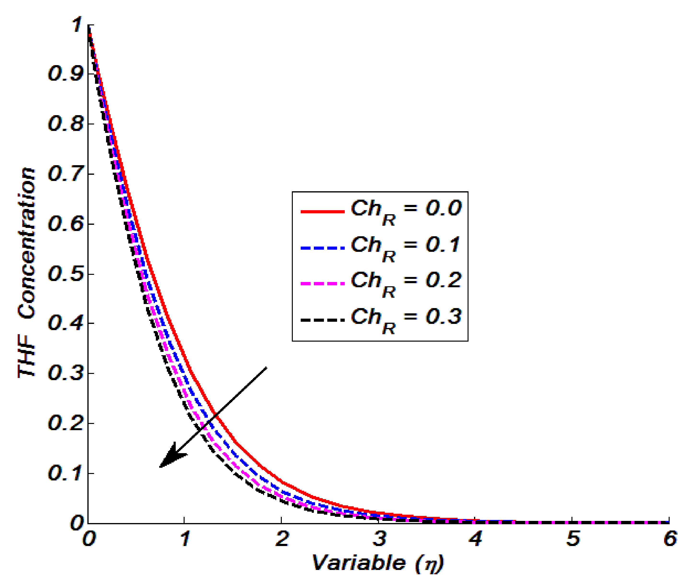
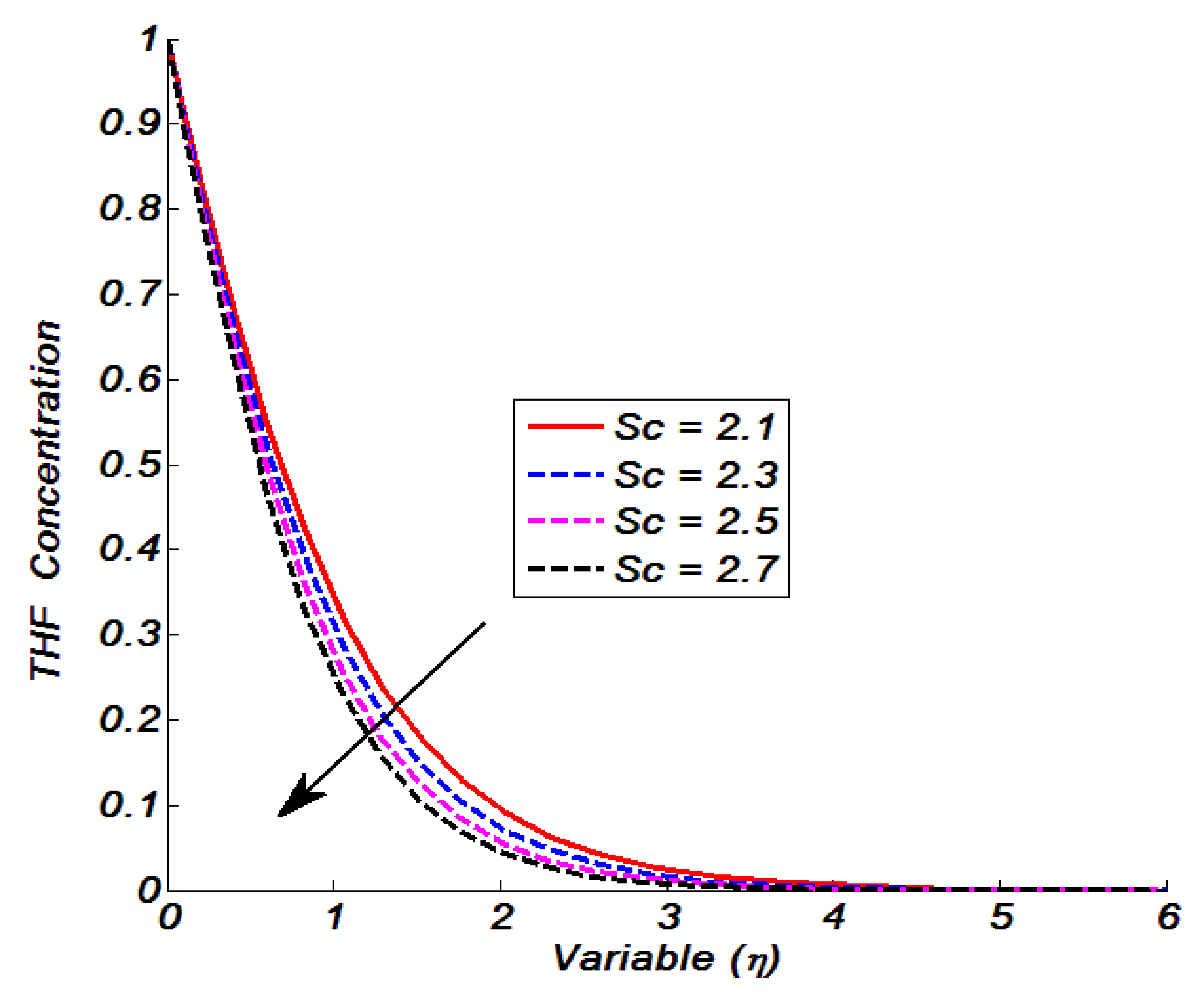
The impact of the chemical reaction and the Schmidt number on the concentration is examined and offered in Figure 1 and Figure 2. Figure 1 depicts the effect of the Schmidt number on the Tangent hyperbolic fluid (THF) concentration; Sc = 2.1, 2.3, 2.5, and 2.7 were used to make this observation. When we raised Sc = 2.1, 2.3, 2.5, and 2.7, we discovered that the concentration drops dramatically. Pr’s effect on the THF temperature is equivalent to this phenomenon. Because Sc and mass diffusivity have an inverse relationship, an increase in Sc induces a decrease in mass diffusivity, which lowers the THF concentration. The fluctuations in concentration for positive values of the chemical reaction parameter are depicted in Figure 2. We discovered that the concentration decreased as the chemical reaction parameter increased, that is $C{h}_R=0.0, 0.1,0.2 \mathrm{and} 0.3.$ One can see that the flow field was non-reactive when $C{h}_R=0.0,$ and that the magnitude of the THF concentration was higher in this case than in reactive flow fields that were $C{h}_R= 0.1,0.2 \mathrm{and} 0.3.$ The variations in Sherwood number in three different frames, namely in the magnetized and non-magnetized flow fields, porous and non-porous materials, and reactive and non-reactive flow fields, are presented in

Table 1. Mass transfer rate values for the magnetized and non-magnetized flow fields.

$\mathit{C}{\mathit{h}}_{\mathit{R}}$	Mass Transfer Rate
	Non-Magnetized Field	Magnetized Field
0.0	−0.2218	−0.2194
0.1	−0.3769	−0.3750
0.2	−0.4924	−0.4909
0.3	−0.5868	−0.5855
0.4	−0.6682	−0.6670
0.5	−0.7405	−0.7395

,

Table 2. Mass transfer rate values for reactive and non-reactive flow fields.

Sc	Mass Transfer Rate
	Non-Reactive Flow	Reactive Flow
2.0	−0.7250	−0.9254
2.1	−0.7498	−0.9444
2.2	−0.7741	−0.9632
2.3	−0.7980	−0.9819
2.4	−0.8215	−1.0004
2.5	−0.8445	−1.0188

and

Table 3. Mass transfer rate values for the porous and non-porous media.

$\mathit{C}{\mathit{h}}_{\mathit{R}}$	Mass Transfer Rate
	Non-Porous Medium	Porous Medium
0.0	−0.2246	−0.2165
0.1	−0.3789	−0.3729
0.2	−0.4940	−0.4891
0.3	−0.5882	−0.5840
0.4	−0.6694	−0.6656
0.5	−0.7417	−0.7382

. For both magnetic and non-magnetized flow fields, Table 1 shows the Sherwood number variations. Such fluctuations were investigated as the value of the variable $C{h}_R$ rise. Here, $M_P=0$ was the non-magnetized condition, and we noted that the mass transfer rate was an increasing function of $C{h}_R$ in the absolute frame. We investigated a magnetized flow field with $M_P=0.3$ and discovered that the Sherwood number grew with the iterations $C{h}_R=0.0,0.1,0.2,0.3,0.4 \mathrm{and} 0.5 .$ The variance in the Sherwood number was similar in both the flow fields, as seen in Table 1. Table 2 shows how the Sherwood number varied in both the reactive and non-reactive flow fields as Sc increased. The Sherwood number increased dramatically when we iterated Sc = 2.0, 2.1, 2.2, 2.3, 2.4, and 2.5 for the non-reactive flow field, that is, $C{h}_R=0.0.$ The scenario of a chemically reactive flow field was implied by choosing $C{h}_R=0.3.$ For Sc = 2.0, 2.1, 2.2, 2.3, 2.4, and 2.5, we noticed that the change in Sherwood number was positive in nature. Aside from that, it is worth noting that the Sherwood number in a reactive flow field was larger than in a non-reactive flow field. The changes in Sherwood number for flow over porous and non-porous materials are seen in Table 3. This observation was made in order to investigate the relationship between the Sherwood number and $C{h}_R.$ In the non-porous medium scenario that is $P_M=0.0$, implied here, we noticed that the Sherwood number grew. For $P_M=0.3$, we used a porous media, and variations in Sherwood number were examined for iterations $C{h}_R=$ 0.0, 0.1, 0.2, 0.3, 0.4 and 0.5. We discovered that varying $C{h}_R=0.0,0.1,0.2,0.3,0.4 \mathrm{and} 0.5$ increased the Sherwood number considerably. Furthermore, we discovered that in the case of non-porous media, the Sherwood number was larger than in the porous medium.

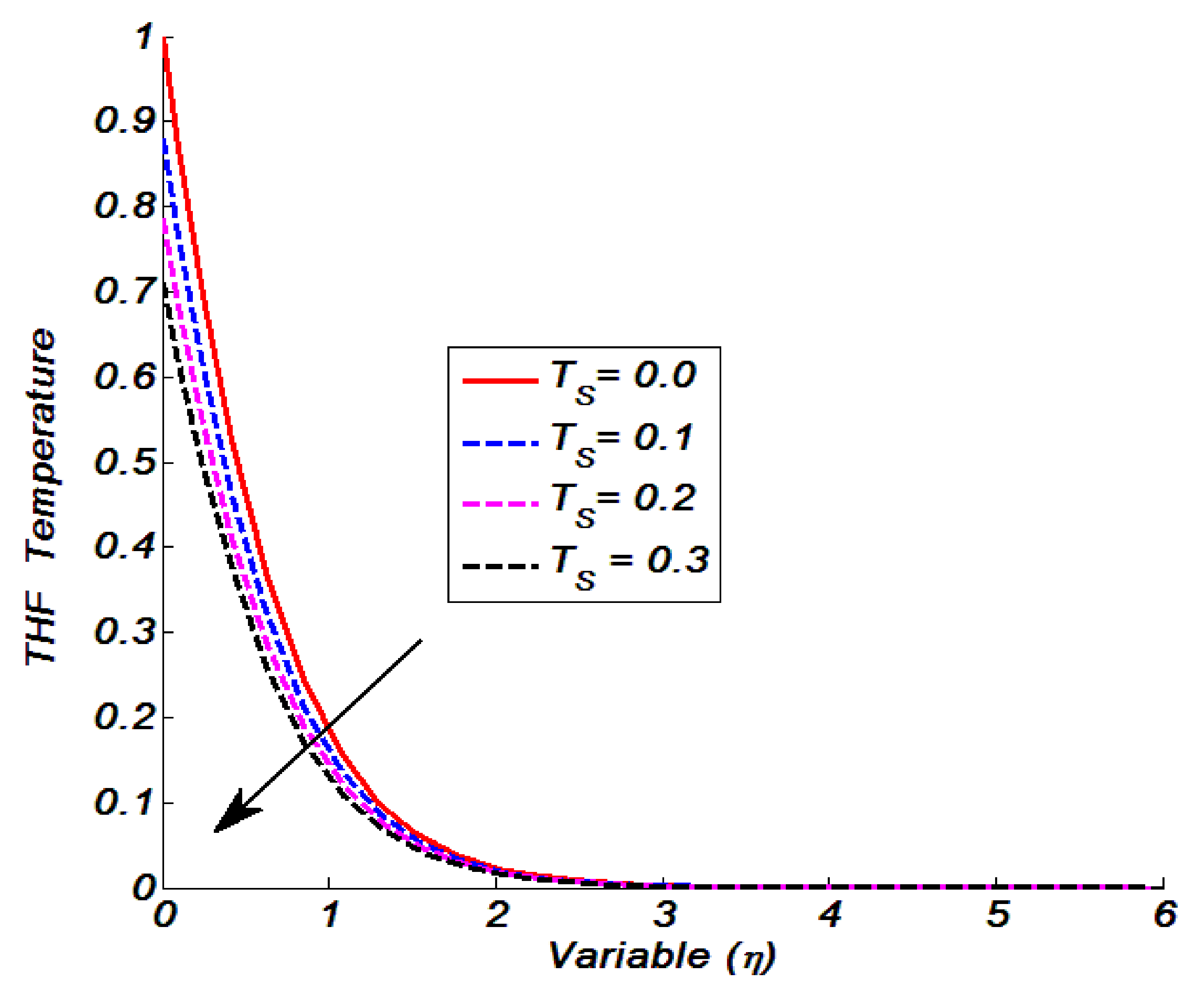
The temperature change is shown against the thermal slip parameter, heat generation, Prandtl number, and heat absorption in Figure 3, Figure 4, Figure 5 and Figure 6. The influence of thermal slip on temperature was examined and is presented in Figure 3. The variables $T_S= 0.0, 0.1,0.2 \mathrm{and} 0.3$ were used to make such observations. In this case, $T_S= 0.0,$ denotes a non-thermal slip flow field, and the temperature magnitude was noticeably higher than in $T_S= 0.1, 0.2, \mathrm{and} 0.3$. We discovered that the THF temperature decreased as the thermal slip parameter increased. 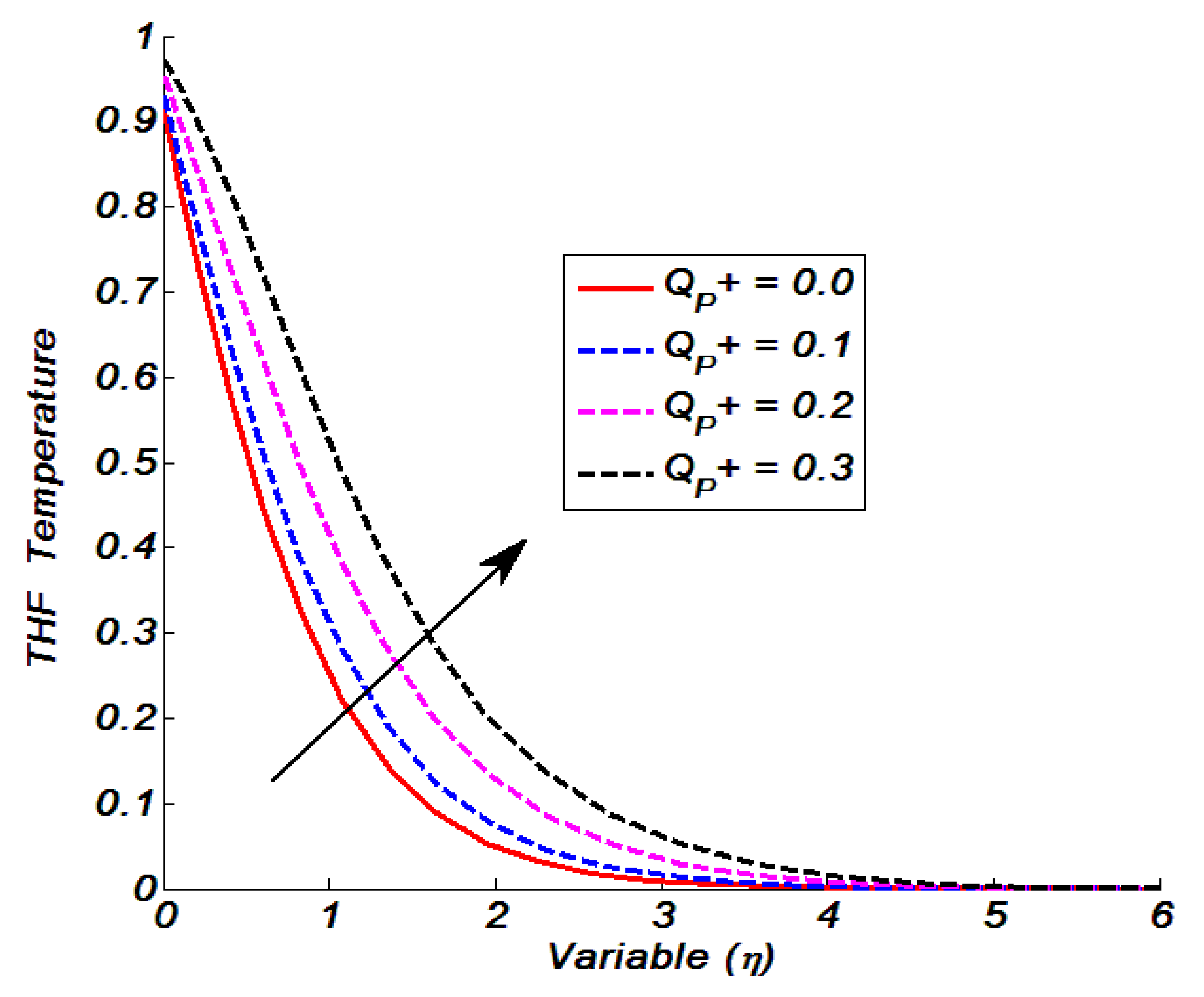The temperature profile is shown in Figure 4 for greater values of the heat-generating parameter. The temperature had higher values as we increased $Q_P+=0.0, 0.1, 0.2 \mathrm{and} 0.3$. This is because as the heat generation parameter is increased, heat energy is produced, and this heat energy produces an increase in thermal energy, causing the THF temperature to rise. 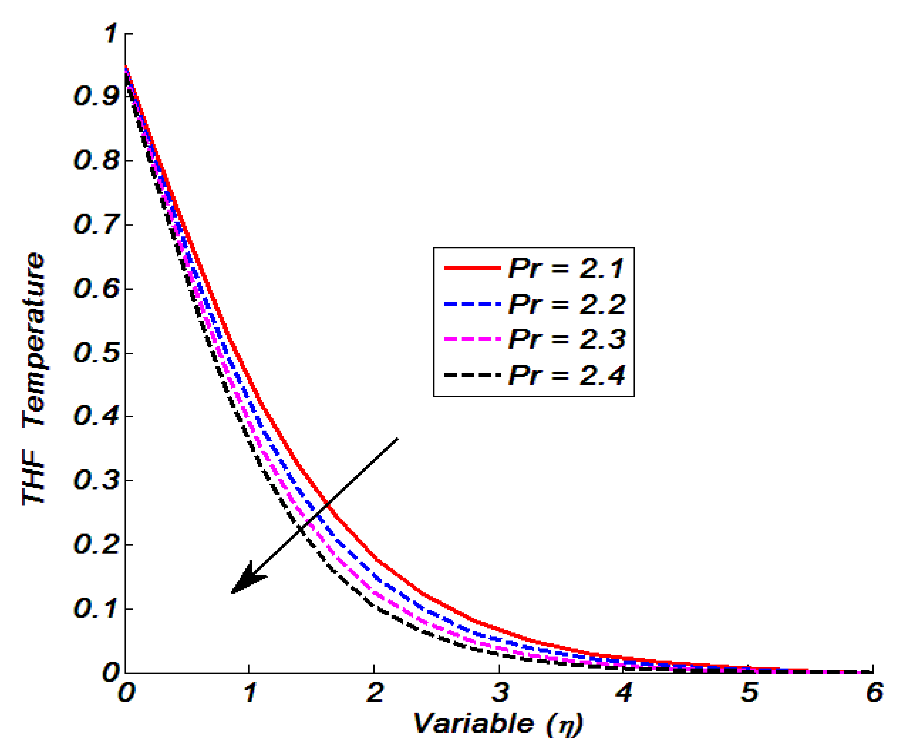Furthermore, we discovered that the temperature of the flow field without a heat source, $Q_P+=0.0,$ was lower than that of the flow field with a heat source: $Q_P+= 0.1,0.2 \mathrm{and} 0.3.$ Figure 5 depicts the effect of a positive Prandtl number fluctuation on the THF temperature. Pr = 2.1, 2.2, 2.3, and 2.4 were used to investigate this impact. The temperature decreased as the value of Pr was increased. Because Pr had an inverse relationship with thermal diffusivity, increasing Pr caused a decrease in thermal diffusivity, lowering the flow field of temperature. 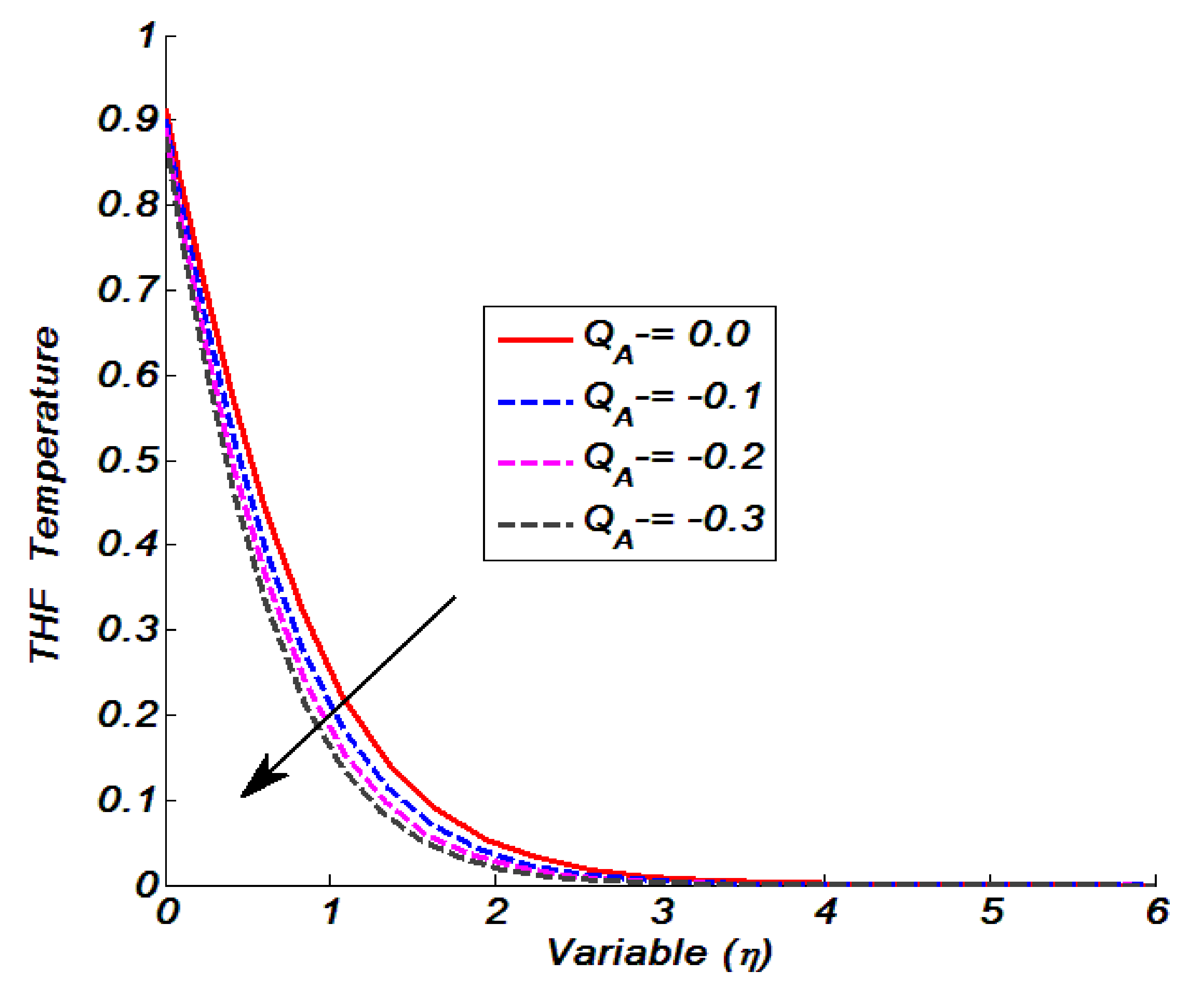The temperature variations towards the heat absorption parameter are shown in Figure 6. The variables $Q_A-= 0.0,-0.1, -0.2 \mathrm{and} -0.3$ were used to make such observations. The temperature appeared to decrease as the heat absorption parameter was increased. This is because negative values of such a parameter represent a heat sink, and in this case, the thermal energy was squandered, resulting in a drop in temperature.

Table 4. Heat transfer rate values for the magnetized and non-magnetized frames.

Pr	Heat Transfer Rate
	Non-Magnetized Field	Magnetized Field
1.0	−0.2905	−0.2943
1.1	−0.3120	−0.3151
1.2	−0.3343	−0.3367
1.3	−0.3571	−0.3588
1.5	−0.4035	−0.3812
1.6	−0.4267	−0.4037

,

Table 5. Heat transfer rate values for the porous and non-porous media.

Pr	Heat Transfer Rate
	Non-Porous Medium	Porous Medium
1.1	−0.3309	−0.2722
1.2	−0.3546	−0.2912
1.3	−0.3785	−0.3110
1.4	−0.4026	−0.3316
1.5	−0.4266	−0.3527
1.6	−0.4504	−0.3741

and

Table 6. Heat transfer rate values for thermal slip and non-slip flow fields.

Pr	Heat Transfer Rate
	Non-Thermal Slip Flow	Thermal Slip Flow
1.1	−0.3199	−0.2919
1.2	−0.3435	−0.3114
1.3	−0.3678	−0.3313
1.4	−0.3926	−0.3513
1.5	−0.4177	−0.3712
1.6	−0.4429	−0.3909

are used to keep track of the Nusselt number variation in three different frames. We measured the numerical values of the Nusselt number in magnetic and non-magnetized frames in the first frame, see Table 4. We presented numerical Nusselt number values in porous and non-porous materials in the second frame, see Table 5. We found numerical values of the Nusselt number in thermal slip and non-thermal slip flow fields in the third frame, see Table 6. In both magnetic and non-magnetized frames, Table 4 shows the effect of positive variations in Pr on Nusselt number; $M_P=0$ was used for non-magnetized flow fields, while $M_P=0.3$ was used for magnetized flow fields. In both cases, the Nusselt number increased for Pr = 1, 1.1, 1.2, 1.3, 1.5, and 1.6 in the absolute frame. Table 5 shows the numerical values of the Nusselt number in porous and non-porous mediums as a function of Pr, with Pr = 1, 1.1, 1.2, 1.3, 1.5, and 1.6. We regarded $W_M=0$ for non-porous, and we entertained $W_M=0.3,$ for porous media. We found that the Nusselt number had a direct relationship with positive Pr values in both circumstances, but that the magnitude of the Nusselt number was bigger in the non-porous media than in the porous material. Table 6 shows the Nusselt number numerical values for Pr = 1, 1.1, 1.2, 1.3, 1.5, and 1.6 in detail. We calculated the Nusselt number for non-thermal slip flow, $T_S=0$, and discovered that higher Pr values resulted in higher Nusselt numbers. We looked into thermal slip flow, $T_S=0.3,$ and found that the Nusselt number increased as Pr increased. Furthermore, when compared to thermal slip flow, the magnitude of the Nusselt number was larger in non-thermal slip flow.

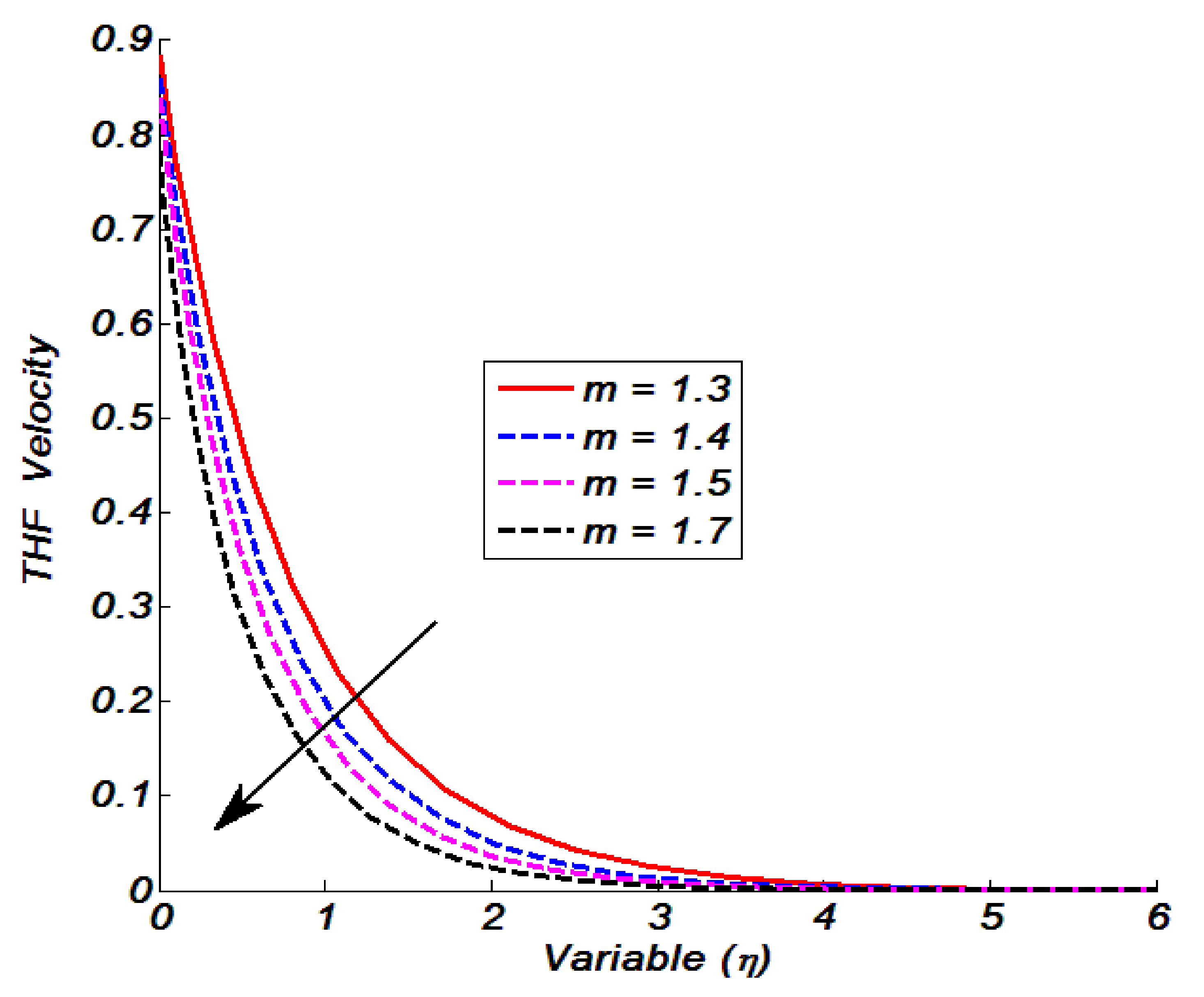
Figure 7, Figure 8, Figure 9, Figure 10 and Figure 11 show THF velocity variations in relation to the power-law index, porosity parameter, magnetic parameter, velocity slip, and Weissenberg number. Figure 7 shows the dependency of THF velocity on the power-law index m. Such observations were noted by varying m = 1.3, 1.4, 1.5, and 1.7. We noticed that when we iterated m = 1.3, 1.4, 1.5, and 1.7, the fluid velocity declined. 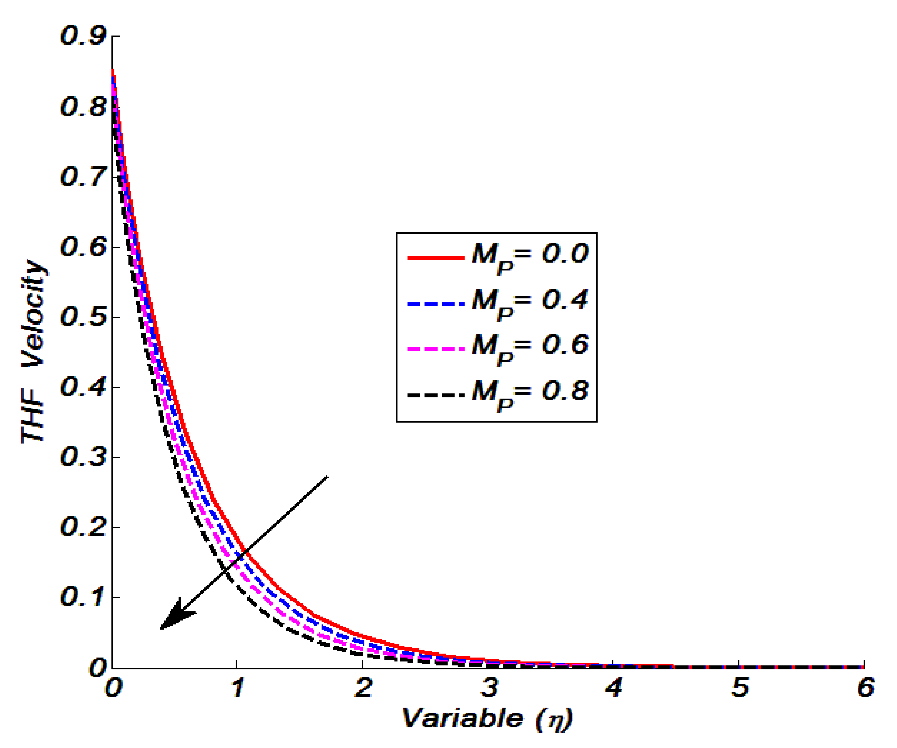Figure 8 is plotted to offer the examination of the THF velocity in relation to the porosity parameter. We saw that when we iterated $P_M=0.0, 0.3, 0.6 \mathrm{and} 0.9$, the THF velocity showed declined values. This is because higher values in the porosity parameter caused lower permeability. Such lower permeability results declined at stretched rates as a result of reductions in velocity. Figure 9 offers the velocity variation in relation to the magnetic parameter. The THF velocity was noted to decrease as a function of $M_P$ = 0.0, 0.4, 0.6 and 0.8. This was because greater $M_P$ boosted the Lorentz force. A boost in Lorentz force gives fluid particles more resistance, and as a result, THF velocity declines. $M_P$ = 0.0 represents the non-magnetized flow field, and the THF velocity magnitude was higher in non-magnetized fields in comparison with $M_P$ = 0.4, 0.6, and $M_P$ = 0.8. The impact of considering velocity slip was examined and is shown in Figure 10. We iterated $V_M= 0.0, 0.1, 0.2 \mathrm{and} 0.3$ and noted the variation in the velocity. We observed that the velocity decreased as a function of the velocity slip parameter. 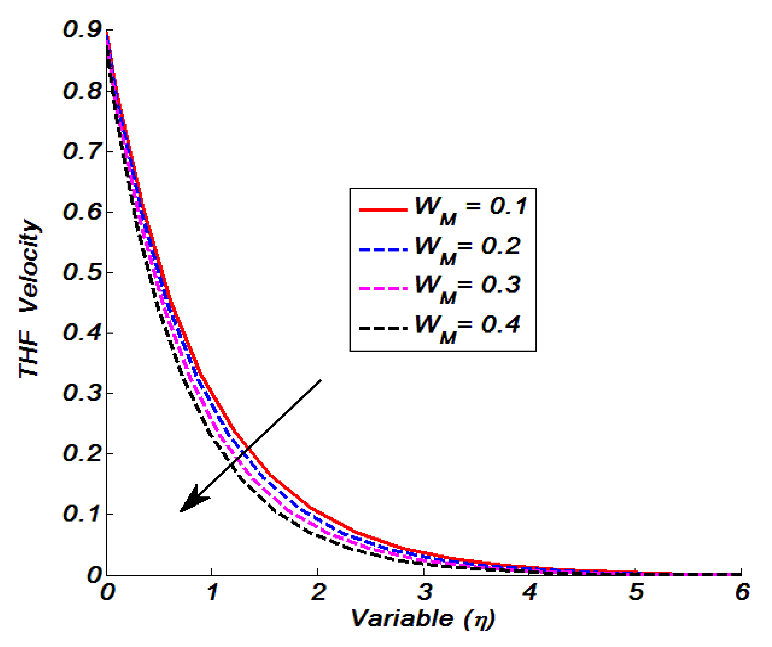Furthermore, one can see that $V_M= 0.0,$ suggested a non-slip flow, and in this case, the velocity magnitude was higher compared to slip flow fields that were $V_M= 0.1, 0.2 \mathrm{and} 0.3.$ Figure 11 shows the influence of the Weissenberg number on the THF velocity. When we iterated $W_M=0.1, 0.2, 0.3 \mathrm{and} 0.4$, the velocity showed a decline. This is because higher values of $W_M=0.1, 0.2, 0.3 \mathrm{and} 0.4$ enhance the relaxation time, which causes an increase in viscosity and Tangent hyperbolic particles faced with higher resistance, which leads to a decrease in the velocity. 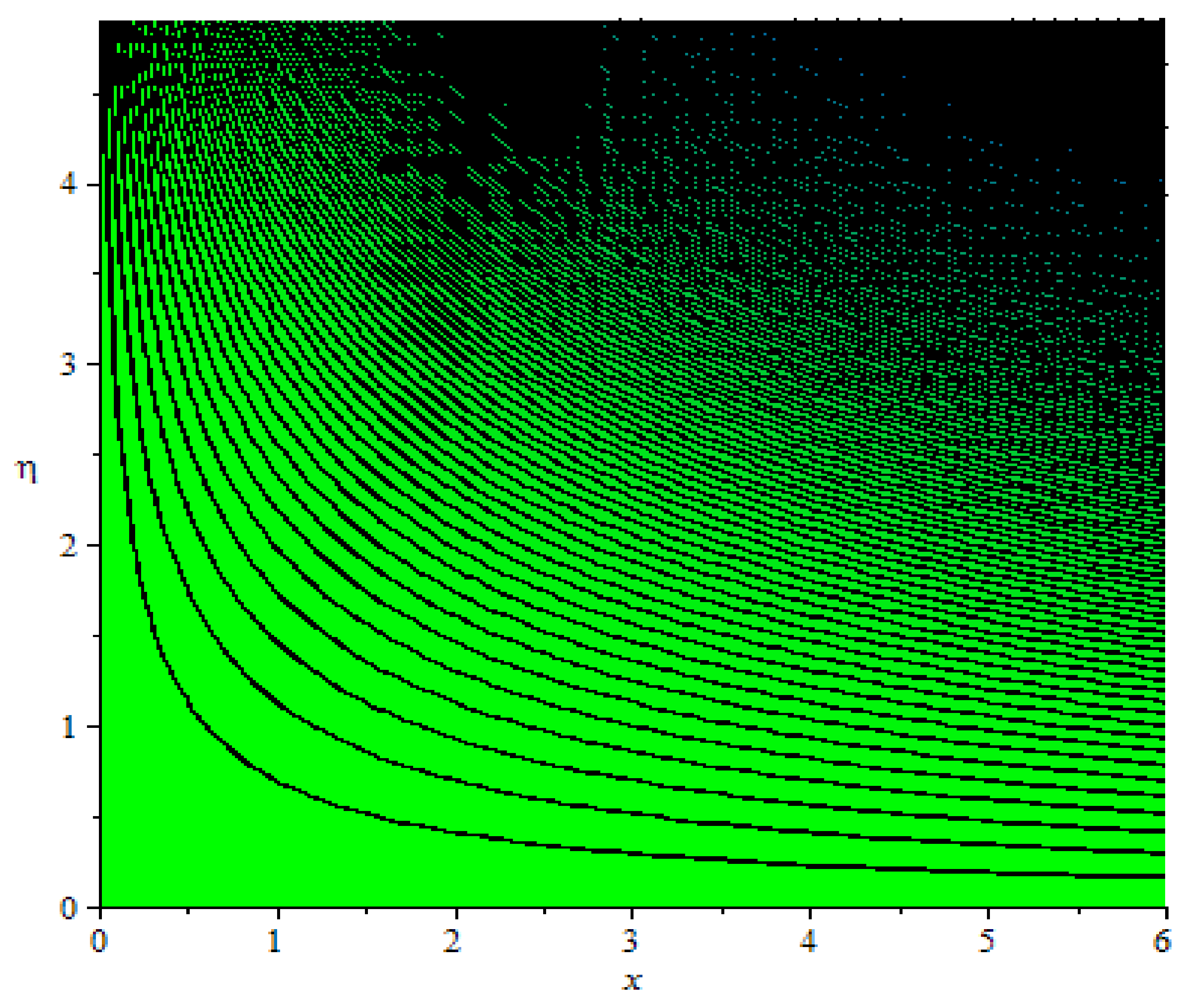Figure 12 and Figure 13 are plotted to offer the fluid flow patterns for both magnetized and non-magnetized flow fields. To be more specific, Figure 12 is the streamlines pattern for the non-magnetized frame, while Figure 13 offers the streamlines pattern for fluid flow in the magnetized frame. It can be seen that in the magnetized frame of reference, the fluid momentum reduced significantly. The skin friction coefficient was calculated by adjusting the power-law index, porosity, and magnetic field parameters in various flow fields. In this area, there are three tables:

Table 7. Skin friction coefficient values for magnetized and non-magnetized flow fields.

m	${\mathit{F}}^{″}(0)$		Skin Friction Coefficient
	Non-Magnetized Field	Magnetized Field	Non-Magnetized Field	Magnetized Field
1.3	−2.1545	−1.6894	0.9481	0.6923
1.4	−1.6103	−1.6894	0.8256	0.8755
1.5	−1.3944	−1.4567	0.8430	0.8875
1.6	−1.2572	−1.3111	0.8808	0.9242
1.7	−1.1578	−1.2064	0.9244	0.9682
1.8	−1.0808	−1.1255	0.9698	1.0144

,

Table 8. Skin friction coefficient values for magnetized and non-magnetized flow fields.

${\mathit{P}}_{\mathit{M}}$	${\mathit{F}}^{″}(0)$		Skin Friction Coefficient
	Non-Magnetized Field	Magnetized Field	Non-Magnetized Field	Magnetized Field
0.0	−1.3226	−1.3874	0.7925	0.8381
0.1	−1.3944	−1.4567	0.8430	0.8875
0.2	−1.4634	−1.5234	0.8923	0.9358
0.3	−1.5300	−1.5881	0.9406	0.9832
0.4	−1.5944	−1.6508	0.9879	1.0298
0.5	−1.6570	−1.7119	1.0344	1.0757

and

Table 9. Skin friction coefficient values for the porous and non-porous media.

m	${\mathit{F}}^{″}(0)$		Skin Friction Coefficient
	Non-Porous Medium	Porous Medium	Non-Porous Medium	Porous Medium
1.3	−1.9799	−1.7928	0.8488	0.7468
1.4	−1.6027	−1.7928	0.8209	0.9421
1.5	−1.3300	−1.5365	0.7977	0.9453
1.6	−1.2011	−1.3799	0.8361	0.9803
1.7	−1.1072	−1.2683	0.8792	1.0245
1.8	−1.0342	−1.1825	0.9236	1.0718

. Table 7 is specifically for measuring the skin friction of THF fluid flow over a porous stretched heated surface. We inspected the impact of the power-law index on the skin friction coefficient in both frames: namely, magnetized and non-magnetized. We observed that when we iterated m = 1.3, 1.4, 1.5, 1.6, 1.7, and 1.8, the skin friction increased significantly. This was the observation for the non-magnetized frame. The same was the case for the magnetized frame, that is, the skin friction coefficient increased towards higher values of the power-law index. It is worth noting that the magnitude of the skin friction coefficient in a magnetized frame was higher than in a non-magnetized frame. For when the changeable variable was the porosity parameter, Table 8 shows the variations in the skin friction coefficient in magnetic and non-magnetic flow fields. We collected the variation in skin friction coefficient by iterating $P_M$ = 0.0, 0.1, 0.2, 0.3, 0.4, and 0.5. In an absolute frame, we can see that the skin friction increased as the porosity parameter increased. Both magnetic and non-magnetized flow fields exhibited this positive fluctuation. When comparing skin friction values in a magnetized flow field to skin friction values in a non-magnetized flow field, the skin friction values for magnetized flow were slightly larger in magnitude. For both porous and non-porous frames, the skin friction coefficient values are listed in Table 9. We investigated the non-porous flow field $P_M=0$ and porous flow field $P_M=0.3$, at higher values of the power-law index m = 1.3, 1.4, 1.5, 1.6, 1.7, and 1.8. For positive values of m, we noted that skin friction increased in the absolute frame. For porous media, similar trends were noticed. For a porous medium, skin friction was much greater than in the case of non-porous medium. We noted that in the absence of mass transfer, velocity slip, and porous medium assumptions, our problem was reduced to the problem studied in Ref. [35]. Here,

Table 10. Comparison of skin friction coefficient with Ref. [35].

${\mathit{M}}_{\mathit{P}}$	m	Ref. [35]		Present Outcomes
		${\mathit{W}}_{\mathit{M}}=0.5$	${\mathit{W}}_{\mathit{M}}=0.3$	${\mathit{W}}_{\mathit{M}}=0.5$	${\mathit{W}}_{\mathit{M}}=0.3$
0.5	0.3	0.96001	0.98804	0.96091	0.98812
1.0	0.3	1.09616	1.13454	1.09635	1.13463
1.5	0.3	1.21235	1.26193	1.21224	1.26181
0	0.0	1.00000	1.00000	1.00001	1.00000
0	0.1	0.93826	0.94248	0.93815	0.94257
0	0.3	0.87026	0.88023	0.87034	0.88017

shows the comparison of skin friction coefficient with the work of Akbar et al. [35]. We found an excellent match, supporting the validity of the present results.

5. Concluding Remarks

A numerical solution is offered for Tangent hyperbolic fluid flow over permeable thermally magnetized surfaces with chemical reaction aspects. The order of flow differential equations is reduced using invariant Lie transformations and then solved by the shooting method. We observed that the concentration of fluid showed an inverse relationship with the Schmidt number and chemical reaction parameter. The mass transfer rate was higher in magnitude for the chemically reactive flow in comparison to the non-reactive flow. The temperature of the fluid showed a direct relationship with the heat generation parameter, while the opposite was the case for the heat absorption parameter, Prandtl number, and thermal slip parameters. Furthermore, the heat transfer rate was significantly high in non-porous mediums as compared to the porous medium. The velocity of the fluid declined in relation to the power-law index, porosity parameter, magnetic parameter, velocity slip, and Weissenberg number. The skin friction coefficient was an increasing function of the power-law index for both porous and non-porous mediums. Besides this, the magnitude of skin friction in a magnetized frame was higher than in a non-magnetized frame.

References

1. Sarma, M.S.; Rao, B.N. Heat transfer in a viscoelastic fluid over a stretching sheet. J. Math. Anal. Appl. 1998, 222, 268–275. [Google Scholar] [CrossRef] [Green Version]
2. Chamkha, A.J.; Issa, C. Mixed convection effects on unsteady flow and heat transfer over a stretched surface. Int. Commun. Heat Mass Transf. 1999, 26, 717–727. [Google Scholar] [CrossRef]
3. Andersson, H.I.; Aarseth, J.B.; Dandapat, B.S. Heat transfer in a liquid film on an unsteady stretching surface. Int. J. Heat Mass Transf. 2000, 43, 69–74. [Google Scholar] [CrossRef]
4. Hou, S.S.; Lin, T.H. Effects of internal heat transfer and preferential diffusion on stretched spray flames. Int. J. Heat Mass Transf. 2001, 44, 4391–4400. [Google Scholar] [CrossRef]
5. Abel, M.S.; Khan, S.K.; Prasad, K.V. Study of visco-elastic fluid flow and heat transfer over a stretching sheet with variable viscosity. Int. J. Non Linear Mech. 2002, 37, 81–88. [Google Scholar] [CrossRef]
6. Bhargava, R.; Kumar, L.; Takhar, H.S. Finite element solution of mixed convection micropolar flow driven by a porous stretching sheet. Int. J. Eng. Sci. 2003, 41, 2161–2178. [Google Scholar] [CrossRef]
7. Zakaria, M. Magnetohydrodynamic viscoelastic boundary layer flow past a stretching plate and heat transfer. Appl. Math. Comput. 2004, 155, 165–177. [Google Scholar] [CrossRef]
8. Khan, S.K.; Sanjayanand, E. Viscoelastic boundary layer flow and heat transfer over an exponential stretching sheet. Int. J. Heat Mass Transf. 2005, 48, 1534–1542. [Google Scholar] [CrossRef]
9. Sanjayanand, E.; Khan, S.K. On heat and mass transfer in a viscoelastic boundary layer flow over an exponentially stretching sheet. Int. J. Therm. Sci. 2006, 45, 819–828. [Google Scholar] [CrossRef]
10. Salem, A.M. Variable viscosity and thermal conductivity effects on MHD flow and heat transfer in viscoelastic fluid over a stretching sheet. Phys. Lett. A 2007, 369, 315–322. [Google Scholar] [CrossRef]
11. Liu, I.-C.; Andersson, H.I. Heat transfer in a liquid film on an unsteady stretching sheet. Int. J. Therm. Sci. 2008, 47, 766–772. [Google Scholar] [CrossRef]
12. Abel, M.S.; Nandeppanavar, M.M. Heat transfer in MHD viscoelastic boundary layer flow over a stretching sheet with non-uniform heat source/sink. Commun. Nonlinear Sci. Numer. Simul. 2009, 14, 2120–2131. [Google Scholar] [CrossRef]
13. Salleh, M.Z.; Nazar, R.; Pop, I. Boundary layer flow and heat transfer over a stretching sheet with Newtonian heating. J. Taiwan Inst. Chem. Eng. 2010, 41, 651–655. [Google Scholar] [CrossRef]
14. Nandeppanavar, M.M.; Vajravelu, K.; Abel, M.S.; Ng, C.O. Heat transfer over a nonlinearly stretching sheet with non-uniform heat source and variable wall temperature. Int. J. Heat Mass Transf. 2011, 54, 4960–4965. [Google Scholar] [CrossRef] [Green Version]
15. Nandeppanavar, M.M.; Vajravelu, K.; Abel, M.S.; Siddalingappa, M.N. Second order slip flow and heat transfer over a stretching sheet with non-linear Navier boundary condition. Int. J. Therm. Sci. 2012, 58, 143–150. [Google Scholar] [CrossRef]
16. Sarif, N.M.; Salleh, M.Z.; Nazar, R. Numerical solution of flow and heat transfer over a stretching sheet with Newtonian heating using the Keller box method. Procedia Eng. 2013, 53, 542–554. [Google Scholar] [CrossRef] [Green Version]
17. Pavithra, G.M.; Gireesha, B.J. Unsteady flow and heat transfer of a fluid-particle suspension over an exponentially stretching sheet. Ain Shams Eng. J. 2014, 5, 613–624. [Google Scholar] [CrossRef] [Green Version]
18. Mabood, F.; Khan, W.A.; Ismail, A.M. MHD boundary layer flow and heat transfer of nanofluids over a nonlinear stretching sheet: A numerical study. J. Magn. Magn. Mater. 2015, 374, 569–576. [Google Scholar] [CrossRef]
19. Li, J.; Zheng, L.; Liu, L. MHD viscoelastic flow and heat transfer over a vertical stretching sheet with Cattaneo-Christov heat flux effects. J. Mol. Liq. 2016, 221, 19–25. [Google Scholar] [CrossRef]
20. Das, K.; Sarkar, A.; Kundu, P.K. Cu-water nanofluid flow induced by a vertical stretching sheet in presence of a magnetic field with convective heat transfer. Propuls. Power Res. 2017, 6, 206–213. [Google Scholar] [CrossRef]
21. Reddy, S.; Naikoti, K.; Rashidi, M.M. MHD flow and heat transfer characteristics of Williamson nanofluid over a stretching sheet with variable thickness and variable thermal conductivity. Trans. A. Razmadze Math. Inst. 2017, 171, 195–211. [Google Scholar] [CrossRef]
22. Jahan, S.; Sakidin, H.; Nazar, R.; Pop, I. Analysis of heat transfer in nanofluid past a convectively heated permeable stretching/shrinking sheet with regression and stability analyses. Results Phys. 2018, 10, 395–405. [Google Scholar] [CrossRef]
23. Jahan, S.; Sakidin, H.; Nazar, R.; Pop, I. Unsteady flow and heat transfer past a permeable stretching/shrinking sheet in a nanofluid: A revised model with stability and regression analyses. J. Mol. Liq. 2018, 261, 550–564. [Google Scholar] [CrossRef]
24. Ali, U.; Rehman, K.U.; Malik, M.Y. The influence of MHD and heat generation/absorption in a Newtonian flow field manifested with a Cattaneo–Christov heat flux model. Phys. Scr. 2019, 94, 085217. [Google Scholar] [CrossRef]
25. Bibi, M.; Zeeshan, A.; Malik, M.Y.; Rehman, K.U. Numerical investigation of the unsteady solid-particle flow of a tangent hyperbolic fluid with variable thermal conductivity and convective boundary. Eur. Phys. J. Plus 2019, 134, 1–14. [Google Scholar] [CrossRef]
26. Hamid, M.; Usman, M.; Khan, Z.H.; Ahmad, R.; Wang, W. Dual solutions and stability analysis of flow and heat transfer of Casson fluid over a stretching sheet. Phys. Lett. A 2019, 383, 2400–2408. [Google Scholar] [CrossRef]
27. Abdelmalek, Z.; Khan, I.; Khan, M.W.A.; Rehman, K.U.; Sherif, E.S.M. Computational analysis of nano-fluid due to a non-linear variable thicked stretching sheet subjected to Joule heating and thermal radiation. J. Mater. Res. Technol. 2020, 9, 11035–11044. [Google Scholar] [CrossRef]
28. Olabi, A.G.; Wilberforce, T.; Sayed, E.T.; Elsaid, K.; Abdelkareem, M.A. Prospects of fuel cell combined heat and power systems. Energies 2020, 13, 4104. [Google Scholar] [CrossRef]
29. Abdelmalek, Z.; Rehman, K.U.; Al-Mdallal, Q.M.; Al-Kouz, W.; Malik, M.Y. Dynamics of thermally magnetized grooved flow field having uniformly heated circular cylinder: Finite element analysis. Case Stud. Therm. Eng. 2020, 21, 100718. [Google Scholar] [CrossRef]
30. Yousri, D.; Abd Elaziz, M.; Oliva, D.; Abualigah, L.; Al-qaness, M.A.; Ewees, A.A. Reliable applied objective for identifying simple and detailedphotovoltaic models using modern metaheuristics: Comparative study. Energy Convers. Manag. 2020, 223, 113279. [Google Scholar] [CrossRef]
31. Naganthran, K.; Hashim, I.; Nazar, R. Non-uniqueness solutions for the thin Carreau film flow and heat transfer over an unsteady stretching sheet. Int. Commun. Heat Mass Transf. 2020, 117, 104776. [Google Scholar] [CrossRef]
32. Uddin, Z.; Vishwak, K.S.; Harmand, S. Numerical duality of MHD stagnation point flow and heat transfer of nanofluid past a shrinking/stretching sheet: Metaheuristic approach. Chin. J. Phys. 2021, 73, 442–461. [Google Scholar] [CrossRef]
33. Rehman, K.U.; Shatanawi, W.; Zahri, M.; Sherif, E.S.M.; Junaedi, H.; Lv, Y.P. Thermal analysis on uniformly heated diamond obstruction in convective liquid suspension. Case Stud. Therm. Eng. 2021, 26, 101062. [Google Scholar] [CrossRef]
34. Ghasemi, S.E.; Hatami, M. Solar radiation effects on MHD stagnation point flow and heat transfer of a nanofluid over a stretching sheet. Case Stud. Therm. Eng. 2021, 25, 100898. [Google Scholar] [CrossRef]
35. Akbar, N.S.; Nadeem, S.; Haq, R.U.; Khan, Z.H. Numerical solutions of magnetohydrodynamic boundary layer flow of tangent hyperbolic fluid towards a stretching sheet. Indian J. Phys. 2013, 87, 1121–1124. [Google Scholar] [CrossRef]
36. Ullah, Z.; Zaman, G.; Ishak, A. Magnetohydrodynamic tangent hyperbolic fluid flow past a stretching sheet. Chin. J. Phys. 2020, 66, 258–268. [Google Scholar] [CrossRef]
Figure 1. Concentration verses Schmidt number.
Energies 14 08530 g001
Figure 2. Concentration verses chemical reaction parameter.
Energies 14 08530 g002
Figure 3. Temperature verses thermal slip parameter.
Energies 14 08530 g003
Figure 4. Temperature verses heat generation parameter.
Energies 14 08530 g004
Figure 5. Temperature verses Prandtl number.
Energies 14 08530 g005
Figure 6. Temperature verses heat absorption parameter.
Energies 14 08530 g006
Figure 7. Velocity verses power law index.
Energies 14 08530 g007
Figure 8. Velocity verses porosity parameter.
Energies 14 08530 g008
Figure 9. Velocity verses magnetic parameter.
Energies 14 08530 g009
Figure 10. Velocity verses porosity parameter.
Energies 14 08530 g010
Figure 11. Velocity verses Weissenberg number.
Energies 14 08530 g011
Figure 12. Streamlines pattern in non-magnetized flow field.
Energies 14 08530 g012
Figure 13. Streamlines pattern in magnetized flow field.
Energies 14 08530 g013