Review

Sensitivity Analysis and Power Systems: Can We Bridge the Gap? A Review and a Guide to Getting Started

E.ON Energy Research Center, Institute for Automation of Complex Power Systems, RWTH Aachen University, 52074 Aachen, Germany
*
Author to whom correspondence should be addressed.
Energies 2021, 14(24), 8274; https://doi.org/10.3390/en14248274
Submission received: 31 October 2021 / Revised: 25 November 2021 / Accepted: 30 November 2021 / Published: 8 December 2021
(This article belongs to the Special Issue Distribution Grid Management Based on the Use of 5G Communication)

Abstract

:
Power systems are increasingly affected by various sources of uncertainty at all levels. The investigation of their effects thus becomes a critical challenge for their design and operation. Sensitivity Analysis (SA) can be instrumental for understanding the origins of system uncertainty, hence allowing for a robust and informed decision-making process under uncertainty. The SA value as a support tool for model-based inference is acknowledged; however, its potential is not fully realized yet within the power system community. This is due to an improper use of long-established SA practices, which sometimes prevent an in-depth model sensitivity investigation, as well as to partial communication between the SA community and the final users, ultimately hindering non-specialists’ awareness of the existence of effective strategies to tackle their own research questions. This paper aims at bridging the gap between SA and power systems via a threefold contribution: (i) a bibliometric study of the state-of-the-art SA to identify common practices in the power system modeling community; (ii) a getting started overview of the most widespread SA methods to support the SA user in the selection of the fittest SA method for a given power system application; (iii) a user-oriented general workflow to illustrate the implementation of SA best practices via a simple technical example.

1. Introduction

Uncertainty, the substance of science [1], pervades the modeling activity of any scientific field; power systems are no exception. Power systems, from planning to operation, from implementation to management, are increasingly affected by various uncertainty sources, e.g., the volatility of newly introduced energy resources (generation, storage, consumption), inaccurate forecasts of weather and load behavior, measurement errors, communication network random delays, incomplete knowledge of component reliability, partial information about the system topology, etc. Investigation of the effects of all relevant uncertainty sources—ultimately impacting the decision-making process—is thus a critical challenge: Sensitivity Analysis (SA) can play a crucial role for its solution by enabling “informed decisions” under uncertainty. Before proceeding further, the general SA framework has to be briefly introduced.

1.1. Sensitivity Analysis: A Quick Glance

1.1.1. Some Useful Definitions

In generic terms, SA studies how—and to what extent—variations in the inputs of a model affect the uncertainty of its output. In this work, the term model is adopted to generically refer to as any numerical procedure or algorithm aiming at reproducing the behavior of a real-world system, to be ultimately used, e.g., for forecast, estimation, calibration, etc. During the building process of a model, a set of “elements” must be defined beforehand: type and structure of the model, model equation parameters, initial and boundary conditions, spatial/temporal resolution levels, forcing data (e.g., time series), alternative scenarios, etc. Each of these elements represents an “assumption” and is inevitably affected by some degree of uncertainty due to, e.g., imperfect knowledge of the model description, data imprecision and/or incompleteness, inherent randomness in the model behavior, etc. The assumptions of interest for the analyst-–which are allowed to vary and be changed prior to model execution so as to assess their impact—are referred to as model input factors (or simply inputs). A rather obvious (though not trivial) consequence of this definition is that, in the context of SA, the analyst can gain no insight into those assumptions that are kept fixed and hence fall outside the set of selected model inputs [2]. The set of all possible combinations of the model inputs’ values is called the input space Ω . By running the model for any particular combination of values of the model inputs, the resulting variable of interest for the analyst is called the model output, which can be, e.g., an objective function, a prediction function, etc. It is noteworthy that often the outcome of interest for the analyst is not necessarily the model output per se, but rather a quantity related to the question the model should try to answer. For example, if the interest is evaluating the performance of a certain voltage control algorithm, the model output to consider would not necessarily be the voltage value at each grid node, but rather some ensemble metrics, e.g., the number of overvoltages.
Given these definitions, it is natural to adopt the following notation:
y = g ( x ) = g ( x 1 , x 2 , , x K )
where y is the model output (scalar, for convenience), x = [ x 1 , x 2 , , x K ] is the vector of the model inputs x 1 , x 2 , …, x K , and g ( · ) is the generic model function, which describes the relationship between the inputs and output. It is noteworthy that g ( · ) might be analytically unknown or mathematically too complex to treat, which is not uncommon in power system applications. In these cases the model is regarded as a “black-box”, i.e., accessible only via simulation by observing the values of the output y produced by querying the model at specific input values ( x 1 , x 2 , …, x K ) .

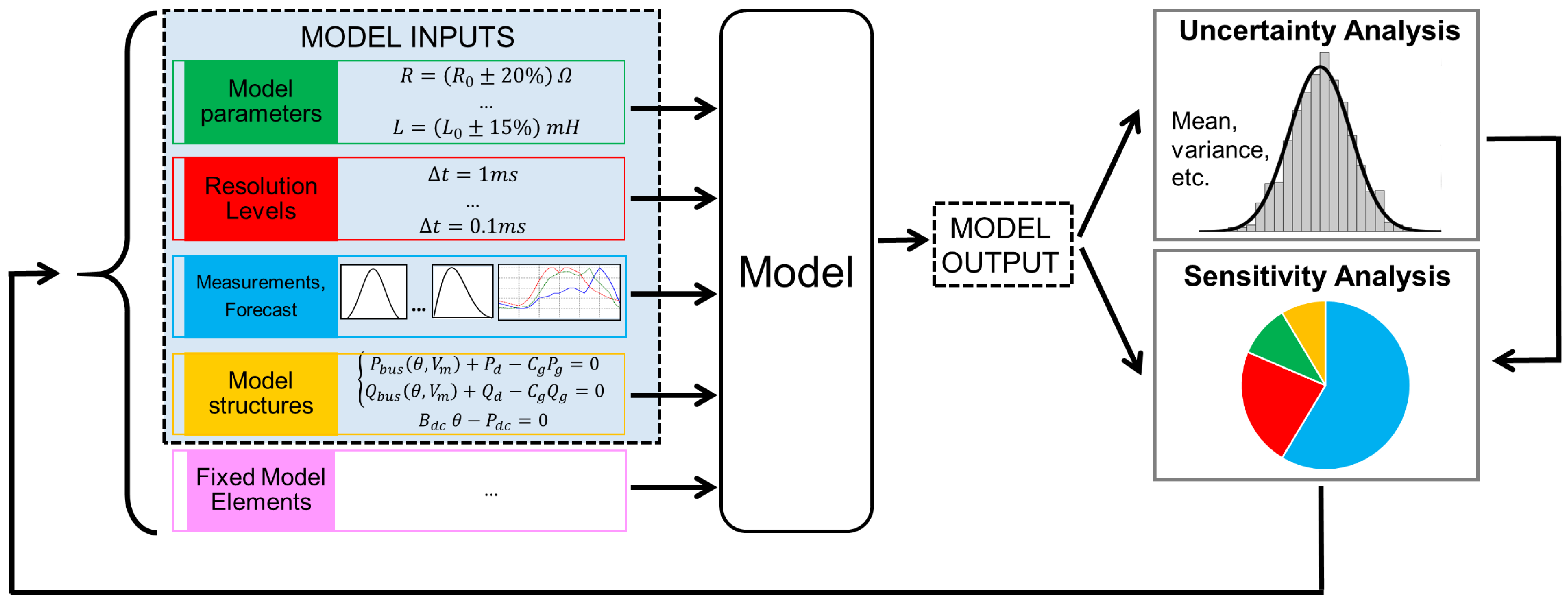
1.1.2. Role of Sensitivity Analysis and Its Connection with Uncertainty Analysis

If appropriately performed, SA is able to efficiently scrutinize model inputs’ uncertainties, hence representing a valuable tool at various levels of the modeling activity (such as model design, validation and control, parameter estimation, prioritization of future research, investigation of the model structure, reduction of model dimensionality, etc.), ultimately being key to building decision-makers’ understanding [3]. The relevance of SA is widely acknowledged also as a model quality assurance tool, and its adoption is even recommended by international regulatory guidelines. For example, in the Impact Assessment Guidelines of the European Commission [4], it is stated that “sensitivity analysis can be used to explore how the impacts of the options you are analysing would change in response to variations in key parameters and how they interact”, whereas according to the United States Environmental Agency [5]: “sensitivity analysis should be used early and often” and “should preferably be able to deal with a model regardless of assumptions about a model’s linearity and additivity, consider interaction effects among input uncertainties, […], and evaluate the effect of an input while all other inputs are allowed to vary as well”. This notwithstanding, SA still experiences some methodological shortcomings when applied by the modeling community, sometimes due to the reluctance to abandon long-established practices [6,7,8]; this applies also with regard to the power system field as demonstrated in this paper.
Exemplary questions that SA can answer are:
  • Which model inputs produce the largest variation in the model output, where, and/or when?
  • Which are the non-influential model inputs that can be confidently excluded from the analysis?
  • Which parts of the input space produce model output values below or above a certain threshold?
  • What is the impact on the model output in response to varying model inputs with respect to a baseline value?
  • Does the model behavior agree with the modeler’s underlying assumptions?
  • In which region of the input space does a specific condition remain optimal?
  • How much would model-based inference change with alternative modeling assumptions?
To fully investigate the effect of all uncertainty sources on the model output (and ultimately on the decision-making process based on it, e.g., in terms of control actions), SA is generally used in combination with Uncertainty Analysis (UA): either analysis represents a valuable complement to the other. UA and SA, although sometimes assuming unclear or even conflating meanings across different disciplines [6], are intended in this paper as distinct—though closely related—activities and are defined as follows [9].
Definition 1. 
Uncertainty analysis is the characterization of the model output uncertainty due to the different sources of uncertainty in the model inputs.
Definition 2. 
Sensitivity analysis is the study of how the uncertainty in the model output can be apportioned to the different sources of uncertainty in the model inputs.
Figure 1 offers a visual description of the UA-SA framework. First, the model inputs to study under the UA-SA framework are defined and their uncertainty is characterized. Then, the model inputs’ uncertainty is propagated forward (e.g., via Monte Carlo simulation) through the model all the way to the output, and its resulting uncertainty can be estimated with UA, e.g., by empirically building a histogram of the output values’ distribution or by extracting some summary statistics such as the mean, variance, median, coefficient of variation, percentiles, confidence intervals, etc. A comprehensive treatment of UA—which is outside the scope of this paper—can be found in [10]. UA stops at the stage of estimating output uncertainty—e.g., to assess whether the model will be functioning within certain specification limits when the model inputs are affected by uncertainty—without practically attributing it to the different model inputs: here is where SA comes into play to identify which modeling assumptions are mainly responsible for the model output uncertainty and, possibly, to what extent, by computing “sensitivity measures” of interest to quantify, e.g., the relative contribution of each model input to the total output uncertainty. Results coming from SA can be used, in turn, as feedback, e.g., to refine inputs’ uncertainty or revise the model definition and iteratively run the whole UA-SA activity.
Ideally, UA is run as a first step (the model output uncertainty needs to be estimated before being apportioned to the different uncertainty sources), and SA is afterwards performed by using information coming from UA to extract the corresponding sensitivity measures. However, various applications exist for which the preliminary UA step is not necessary, but the focus is immediately towards SA (e.g., in the context of model calibration, optimization, and control theory).

1.1.3. Why So Many Sensitivity Analysis Techniques?

By quickly glancing at the content table of any SA handbook (e.g., [9,10,11,12,13]), it is evident that the literature offers a plethora of SA methods among which non-specialist users may easily get lost trying to choose the fittest for their problem. Although SA ultimately consists of a simple “perturb-and-observe” approach—where the model input values are repeatedly changed and the effect on the model output is evaluated—the vast set of SA techniques originates in an elementary argument. In fact, unless the analyst’s interest simply lies in evaluating the effects of small variations of a restricted set of model inputs, the exploration of the whole model input space is revealed to be a hard task if not supported by “smart” sampling strategies (i.e., how the model inputs are perturbed, or “sampled”, to observe the model behavior). Consider a hypothetical model with ten inputs, each of them assuming three different values or “levels” (e.g., minimum, mean and maximum value), for example a microgrid with ten connected energy sources such as photovoltaic systems, wind farms, energy storage systems, etc., each of them with three different penetration levels (e.g., 0%, 50%, 100%) in the context of a network stability study. By using a brute-force (also known as “grid search”) approach, the study of all input levels’ combinations would imply running the model already at almost 60,000 combinations. Intuitively, when the model dimensionality (i.e., the number of model inputs) becomes progressively higher and the model input uncertainty shall be studied more thoroughly than by considering just a small set of levels, the complexity of the SA problem can quickly—and often dramatically—increase (because of the so-called “curse of dimensionality”), with the brute-force approach becoming quite hopeless. Therefore, over the recent years, SA practitioners have constantly been engaging in developing more and more sophisticated SA techniques—often leveraging the specific features of their own application area—in the attempt to find a good balance between SA informative content and acceptable computational load under a resource-saving context. Not surprisingly, SA has its roots in the “Design of Experiments” (DoE) theory dating back to the early 20th Century [14], which encompasses different statistical methods for efficiently laying out a thorough plan in advance of carrying out (potentially time-expensive) experiments.

1.1.4. Classification of Sensitivity Analysis Methods

SA methods can be classified into “local” or “global” under the input space exploration viewpoint and into “One-At-a-Time” (OAT) or “All-At-a-Time” (AAT) according to the adopted sampling strategy [9,15]:
  • Traditionally, it has been common practice across the scientific community, not only in the power system area, to adopt local SA approaches (e.g., [16,17,18,19,20]). In local SA, input variability is studied around just a specific baseline point x 0 , with the model inputs being varied over a small neighborhood (“locally”, indeed) around x 0 , which is usually the user’s operational/nominal point or what is believed to be the “appropriate” or “best known” configuration. Consequently, local sensitivity measures (such as y x i , i.e., the model output partial derivative with respect to each of the model inputs), are dependent on the specific input space location x 0 at which they are computed. On the other hand, global SA approaches aim at exploring (at least conceptually) the whole input space, i.e., by encompassing the full range of model inputs’ variability and not only the neighborhood of x 0 [21]. It is worth noting that the applicability of local SA is valid only for “small” changes, and it is limited to just a small neighborhood around x 0 , unless the model is proven to be linear in all its inputs (whereby y x i remains constant for any x 0 ). Importantly, if the model is nonlinear to a certain degree or large uncertainty affects the model inputs, as is often the case in power systems, local SA provides only an incomplete view of model sensitivity behavior and might offer misleading information when used for speculating upon model sensitivity behavior at a “global” level. On the other hand, global SA, though being generally more expensive than local SA, allows for the full accounting of model inputs’ uncertainty by pursuing a complete exploration of the input space;
  • Besides the distinction between global and local, SA methods can be divided between OAT and AAT according to the sampling strategy viewpoint. In OAT approaches, the model inputs are varied one by one, in turn, while keeping all the others fixed at their baseline values. In AAT approaches, instead, the model inputs are simultaneously varied, e.g., as Monte Carlo simulations. The OAT sampling strategy is by far the most popular approach applied in SA, probably due to its inherent simplicity and intuitiveness [6,8]. In fact, changing one input at a time while holding all other inputs constant logically implies that whatever observed effect on the model output can be uniquely attributed to the specific perturbed input. However, as further discussed in Section 2, OAT approaches—though well matched to the analyst’s intuitive way of thinking—suffer from a major drawback: due to their nature, they cannot detect the presence of model inputs’ interactions, which thus remain unexplored. In other words, OAT strategies can reveal only the individual contribution of a given model input, whereas higher-order effects are allowed to emerge only via AAT designs, i.e., by moving (perhaps counter-intuitively at first glance) more than one input at a time.

1.1.5. Remark on Local and Global Sensitivity Analysis

Generally, local SA methods adopt OAT approaches, whereas global SA methods may utilize either OAT or AAT sampling strategies. From the previous discussion, it follows that local/OAT SA methods might not yield a full insight into the “true” effect of model inputs’ uncertainty, apart from particular circumstances (e.g., linear models) where the local sensitivity behavior of the model is informative also at a global level. However, local SA approaches are not wrong per se: there is plenty of literature across different scientific disciplines adopting, e.g., derivative-based methods (such as adjoint methods [13], gradient-based optimization [22], differential importance measures [23], tolerance analysis for linear programming [24], etc.), and the availability of, e.g., automated differentiation methods [25,26] is an invaluable tool especially for large-dimensional systems. In fact, sometimes, the analyst’s research question can be oriented toward investigating what happens in the vicinity of a somehow “optimal” or “predetermined” point of interest (e.g., to study the effect of infinitesimal perturbations around a baseline), or other times, the model at hand features some linearity degree, thus ensuring the sensitivity measure values remain reasonably constant over the model input space. In these situations, resorting to local SA methods might be a justified choice. However, problems start arising when local SA is improperly used, e.g., to assess the relative importance of model inputs in the presence of (finite ranges of) uncertainty: in these circumstances, as the input/output relationship becomes less linear, the effectiveness of local sensitivity measures decreases to the point where they can even totally fail to spot important model inputs. Since SA is often used as a support tool by analysts, modelers, and (more broadly) stakeholders, the adoption of inaccurate or low-informative SA might ultimately affect the consequent decision-making process [27].

1.1.6. Desirable Features of Sensitivity Analysis

As noted in [9], desirable properties that should characterize an SA method are:
  • Ability to cope with scale/shape effects, i.e., incorporation of the whole variation range of the inputs and their distribution;
  • Inclusion of multidimensional averaging, i.e., exploration of the input space at a global scale by simultaneously varying all inputs so as to let potential interactions emerge;
  • Independence from any prior assumption on the model form, i.e., possibility to apply—and, more importantly, trust—the sensitivity measure regardless of the validity of specific model properties (an SA method possessing this property is “model-free”);
  • Ability to deal with groups of model inputs, i.e., capacity to treat sets of inputs as if they were single inputs to facilitate the agility of result interpretation.
SA methods that own these features (such as the variance-based SA techniques described in Section 2.3.3) are capable of effectively studying how and how much the model output is affected by the different model inputs’ uncertainty (both individually and through interactions among them), thus offering an in-depth exploration of the model sensitivity behavior and providing more defensible results, as well as sturdy conclusions [28,29].

1.2. Sensitivity Analysis for Power Systems

SA has a long tradition in the power system field [30,31]. SA applications can be recorded in a variety of contexts, e.g., voltage control [32,33,34,35,36,37], frequency support [38,39], reliability analysis [19,40,41], voltage stability analysis [42], network planning [43,44], design [45,46] and reconfiguration [47], transient analysis [48,49], energy sources optimization [50,51], and optimal device placement [52]. Traditionally, SA has been largely performed by adopting linear techniques, such as the adjoint network method [53,54], Jacobian method [55], and trajectory sensitivity [48], ultimately leading to derivative-based sensitivity coefficients, which have been widely adopted in modern power system engineering. Quite widespread are also more general “perturb-and-observe” approaches [56,57], based on changing model inputs with small perturbations (e.g., varying active and reactive power injections by a fixed fraction of their nominal values) and observing their effect on some quantity of interest (e.g., the voltage magnitude at a specific bus). Both linear techniques and perturb-and-observe approaches fall into the category of local SA and study the system behavior around a specific operating point (for static systems) or trajectory (for dynamic systems), ultimately relying on first-order approximations. Despite their proved efficiency in many power system applications, these local SA methods capture the effect of small changes only around a specific baseline. Therefore, they might be inaccurate when the system is affected by large uncertainty and nonlinearities (e.g., interactive effects) as in today’s power systems due, e.g., to the increasingly large penetration of renewable energy sources and power electronics components, as well as to the complexity of system control architectures. When the exploration of the inputs’ full uncertainty range is of interest and model linearity assumptions are unjustified or too unrealistic to hold, local SA might produce even drastically different baseline-dependent results (as demonstrated in Section 2.2 via a simple exemplification) and, hence, turns out to be inappropriate and not sufficiently informative for completely describing the system sensitivity behavior. To overcome these pitfalls, global SA is the suggested choice. However, despite its undoubted potential for the study of complex power systems under uncertainty, the adoption of global SA is still limited in the power system community, starting to receive more attention only in the last decade [39,58,59,60,61,62].

1.3. Motivation and Objectives of the Paper

This paper is motivated by the following considerations:
  • There is a widely common conviction—see, e.g., the recent position paper [63] by a multidisciplinary authorship team with expertise in SA—that the benefits of SA, despite its wide potential, are not yet fully realized and its role in supporting modelers and experimenters is often not fully exploited across the different research fields. As demonstrated in this paper, this applies also to the power system community, due not only to terminology problems (e.g., what is really meant by “sensitivity analysis”), but supposedly also to the plethora of techniques available for performing SA, among which the (potentially beginner) SA user might easily get lost, remaining doubtful about the most suitable method for the application at hand;
  • Although other SA reviews are available in different research fields (e.g., in the context of chemical [64], environmental [15], Earth-system [65], and hydrological [66] modeling), to the best of the authors’ knowledge, a thorough and up-to-date literature review on the usage of SA methods within the power system modeling community is missing;
  • Unlike local SA, global SA techniques are undoubtedly less spread throughout the power system modeling community, being sometimes improperly applied or not even known (maybe because of partial communication among SA practitioners and SA final users, the relatively young age of global SA, the lack of statistical training, or the absence of discipline-specific application examples [6,27,63]).
Accordingly, the goals of the present review paper are:
  • To provide (in Section 2) an introductory overview of the main SA methods available to the power system community, with particular focus on methodological bases, properties (weaknesses and strengths), and applicability boundaries, ultimately guiding the user in the best-fitting SA technique quest for the problem of concern;
  • To present (in Section 3) a gap-filling systematic and critical literature review of the SA practice state-of-the-art in the power system field, with a suggested high-level categorization of power system applications according to the SA framework;
  • To furnish (in Section 4) a ready-to-use and operational-oriented general workflow with illustration of the recommended steps for running global SA and a discussion of the user’s relevant choices.
Additionally, the overarching aim of this paper is bridging the gap between power system experts and the SA realm, ultimately triggering a discussion on (and awareness of) SA within the power system community.

1.4. Intended Audience for the Paper

On the one hand, the present paper targets all power system researchers and practitioners, providing them with: (i) a detailed discipline-specific literature review of SA practices; (ii) a concise, but effective description of the most widely used SA methods with detailed references for further engaging with the SA literature; (iii) a ready-to-use general workflow in the form of a technical tutorial to guide in the operative application of global SA (possibly promoting its routine adoption). On the other hand, SA researchers can find in this paper an up-to-date presentation of the state-of-the-art of SA methods in the power system field, as similar review works have done with regard to other research fields [15,64,65,66]. It is worth saying that this literature review work is considered to be representative of the status quo of SA in the power system sector, though without claiming to be comprehensive.

1.5. Structure of the Paper

The remainder of this paper is organized as follows. Section 2 offers an operative review of some selected SA methods. Section 3 describes the bibliometric study carried out to analyze the SA status quo within the power system field and provides the corresponding outcomes. Section 4 illustrates a practical general workflow for running global SA with the help of a technical example. Section 5 presents provides a list of operative hints for adopting SA. Section 6 concludes the paper.

2. Operative Review of Sensitivity Analysis Methods

This section provides a review of the most widely adopted SA methods in power system applications as a result of the bibliometric study presented in Section 3. The reviewed SA methods are presented following the local/global categorization and are summarized in Table 1. The mathematical details are minimized, and instead, focus is put on an intuitive description of the methodology, operational properties (including cost of the analysis), and applicability limits of the reviewed SA methods. A “toy function” is used for exemplification throughout the section.

2.1. The Toy Example

The toy example adopted throughout Section 2 is described hereafter. It is noteworthy that the motivation for adopting a simple analytical example (purposely released from any specific power system application) is threefold. First, it shows the specific SA method at work, helping the (potentially SA beginner) reader to better understand it. Second, the self-evident sensitivity pattern of the toy model enables the reader to intuitively infer beforehand the behavior of its output as a function of the model inputs, hence allowing the comparison of each SA method outcome with the reader’s preliminary expectation. Third, the simplicity of the toy function enables discussing in quantitative terms how the specific SA method behaves in the case that its underlying assumptions are not verified, ultimately allowing a straightforward evaluation of the errors arising therefrom (e.g., in terms of wrong model inputs’ ranking, missed detection of interactive effects, etc.)
As a toy example, consider the following model g ( x ) :
y = g ( x ) = x 1 2 x 2 + 4 x 1 x 3
where y is the scalar model output and x = [ x 1 , x 2 , x 3 ] is the vector of model inputs. This model is assumed to be deterministic, i.e., whenever the model inputs are set to a specific value x 0 , the resulting model output always assumes the same value y 0 = g ( x 0 ) . The focus of this paper is on deterministic models only, whereas stochastic models—in which a random value of y is obtained whenever the model inputs are set to x 0 as, e.g., in the case of agent-based models—are not considered. SA in the context of stochastic models was tackled, e.g., in [67,68].
Despite its apparent simplicity, the structure of the model in Equation (2) is characterized by a combination of “relevant” functions: a quadratic term, a negative linear term, and an interactive term. Formally speaking, this model is nonlinear (due to x 1 2 and x 1 x 3 ) and non-additive (due to x 1 x 3 ). As such, it is intended to broadly represent a wide set of power systems’ typical functions (without representing a specific one of them), e.g., the power balance equations of a power flow problem, the synchronous machine models and associated control systems, the current–voltage relationships of power electronic components (e.g., diodes, transistors), etc.
The three model inputs are considered to be uncertain to reflect—in general terms—the randomness affecting today’s power systems, where, e.g., circuit elements are manufactured with tolerances, circuit component failure/repair rates can only be estimated, forecast and measurements are affected by errors or uncontrollable variability, high volatility energy resources (such as renewable and consumer-owned sources) are introduced in the energy mix, etc. In particular, imagine that the “true” values of x 1 , x 2 , x 3 are not exactly known by the analyst and the following plausible ranges of variation are defined: x 1 [ 0.5 , 0.5 ] , x 2 [ 0.5 , 1.5 ] , x 3 [ 0 , 1 ] . Consider just the minimum ( x i ) and maximum ( x i + ) values for each model input to be sufficient for performing all the local SA methods reviewed in Section 2.2, since they are performed under a deterministic framework, i.e., without the requirement to assign specific Probability Density Functions (PDFs) to the model inputs: any value between x i and x i + is a possible value of x i , without a specific probability information associated to it. However, when turning to global SA methods, a probabilistic framework has to be adopted by considering PDFs that reflect the analyst’s uncertain knowledge about the model inputs. Hence, for the global SA methods reviewed in Section 2.3, assume that the model inputs are independent (i.e., with null correlation) with the following PDFs: X 1 U [ 0.5 , 0.5 ] , X 2 U [ 0.5 , 1.5 ] , X 3 U [ 0 , 1 ] , where the capital letters X i indicate that the model inputs are considered as random variables, the symbol “∼” stands for “distributed as”, and U indicates the uniform PDF (i.e., each value of X i has the same probability 1 x i + x i of occurring between x i and x i + ).

2.2. Local Sensitivity Analysis Methods

Local SA is often performed by taking into account a deterministic framework, with no need to specify a PDF for the model inputs. Local SA, mainly adopting OAT approaches, examines the impact of reasonably small changes only in base case assumptions and could be chosen when the analyst is purely interested in investigating the model output sensitivity just around a predetermined point of interest (often called base case x 0 ), even assuming that the model inputs are uncertain and vary between plausible ranges. In this section, four deterministic local SA methods are reviewed: Tornado diagram, one-way SA, scenario analysis, and differential SA.

2.2.1. Tornado Diagram

Probably the most elementary SA method is represented by the so-called “Tornado diagram” [69], which is based on OAT designs and is often preferred for its simplicity of calculation, as well as for its capability to display SA results in an effective and immediate way [70,71,72].
In a Tornado diagram, each model input takes generally three distinct values (or “levels”): two extreme values and a base case value. The procedure starts with choosing a base case x 0 . Plausible ranges for the inputs’ variation are also defined and two endpoints are specified: x + = [ x 1 + , x 2 + , , x K + ] and x = [ x 1 , x 2 , , x K ] . The components of the vectors x + and x are the upper and lower values of the model inputs, respectively. Each input is then moved OAT from the base case to its upper value (keeping all the others fixed at their base case) to obtain the point ( x i + , x i 0 ) with coordinates [ x 1 0 , x 2 0 , , x i + , , x K 0 ] , where only x i has been shifted from x i 0 to x i + . The notation “ i ” stands for “except i”: x i 0 hence indicates that all inputs but x i are kept fixed to the base case values.
Given the base case x 0 and the point ( x i + , x i 0 ) , it is possible to calculate the sensitivity measure Δ i + y , i.e., the variation Δ of the model output y due to changing alone the model input x i from x 0 to ( x i + , x i 0 ) :
Δ i + y = g ( x i + , x i 0 ) g ( x 0 )
This is repeated, in turn, for all the model inputs, and the variations in the model output to individual changes of the model inputs are recorded. The procedure continues by moving each input OAT from the base case x i 0 to its lower limit x i and then taking the difference between the corresponding model output values:
Δ i y = g ( x i , x i 0 ) g ( x 0 )
At the end of the procedure, two sets of OAT sensitivity measures are collected for each model input (i.e., Δ i + y in Equation (3) and Δ i y in Equation (4)). The two sets of OAT sensitivity measures are then plotted in a Tornado diagram as horizontal bars (usually sorted in descending order of magnitude), quickly highlighting those inputs to which the model output is most sensitive. To perform a complete Tornado-diagram-based SA, the total computational cost is quite limited: only 2 K + 1 model runs are required (where K is the number of model inputs).
For our toy example, assume that the base case is x 0 = [ x 1 0 , x 2 0 , x 3 0 ] = [ 0 , 1 , 0.5 ] , whereas the two endpoints are x + = 0.5 , 1.5 , 1 and x = 0.5 , 0.5 , 0 . By varying each input individually from the base case to its upper value, the following shifts Δ i + y are obtained:
Δ 1 + y = g 0.5 , 1 , 0.5 g 0 , 1 , 0.5 = 1.25 Δ 2 + y = g 0 , 1.5 , 0.5 g 0 , 1 , 0.5 = 0.5 Δ 3 + y = g 0 , 1 , 1 g 0 , 1 , 0.5 = 0
Afterwards by varying each input individually from the base case to its lower value, the following shifts Δ i y are obtained:
Δ 1 y = g 0.5 , 1 , 0.5 g 0 , 1 , 0.5 = 0.75 Δ 2 y = g 0 , 0.5 , 0.5 g 0 , 1 , 0.5 = 0.5 Δ 3 y = g 0 , 1 , 0 g 0 , 1 , 0.5 = 0
Finally, the two sets of OAT sensitivity measures Δ i + y and Δ i y are plotted in a Tornado diagram, as shown in Figure 2.
The information provided by the Tornado diagram is twofold. On the one hand, insight is given into the direction of output change due to a variation in each of the model inputs alone. According to Figure 2, a 50% increase of x 1 , x 2 , and x 3 with respect to their base cases causes a positive ( x 1 0 x 1 + ), negative ( x 2 0 x 2 + ), and null ( x 3 0 x 3 + ) effect on the model output y, respectively. Conversely, a 50% decrease in each of the three model inputs produces a negative ( x 1 0 x 1 ), positive ( x 2 0 x 2 ), and null ( x 3 0 x 3 ) effect, respectively. On the other hand, the analyst can gain understanding about the magnitude of the effect on the model output due to equal changes in the individual inputs: in a hypothetical importance ranking of the model inputs, x 1 would stand out as the “winner” followed by x 2 , with x 3 having a null effect.
One point bears consideration. According to Figure 2, since both Δ 3 + y and Δ 3 y are null, the analyst would be prone to infer that the model output is not affected at all by the variation of x 3 (in neither direction): this is quite at odds with the expectations. In fact, by recalling the toy example function, x 3 does appear in Equation (2); hence, it should play some role. A further confirmation that something is going wrong comes from a simple consistency check. By evaluating the model at the upper endpoint x + = [ x 1 + , x 2 + , x 3 + ] =   0.5 , 1.5 , 1 (i.e., when all the three inputs are moved, simultaneously, to their upper values) and by computing the difference between the model output evaluated at x + and the base case x 0 , the result is g ( x + ) g ( x 0 ) = 1.75 . Unfortunately, a different result is obtained by summing up all the individual variations in the model output due to OAT input increments: Δ 1 + y + Δ 2 + y + Δ 3 + y = 0.75 . Where does this difference come from? It is sufficient to recall the toy example function for realizing that the interactive term involving x 3 is the missing part, which is not captured by the Tornado diagram. This intuitively demonstrates one well-known limitation of, in general, all OAT SA techniques: due to its nature, an OAT sampling strategy keeps the model interactions “dormant”, and the analyst might run into the risk of considering as non-influential one model input that instead does play a role (as x 3 in this case). In classical statistical theory, this is known as “Type II error”, i.e., erroneously classifying an important input as non-influential [73]. To circumvent this issue, the so-called generalized Tornado diagrams were introduced in [74] by combining standard Tornado diagrams with scenario analysis (see Section 2.2.3) so as to reach a decomposition of the model output change through a finite number of higher-order terms.
To summarize, SA based on Tornado diagram is inexpensive (in terms of computational cost), intuitive, and easy to implement, hence being quite attractive to the analyst. However, the drawn conclusions (e.g., in terms of input importance ranking and the direction of output change) are limited to the specific input space location where the model is evaluated (i.e., the base case) and are valid only for the specific perturbations applied to each individual input (e.g., the variation between the two endpoints), while holding the other inputs at the base case. Moreover, since no interactive effects among inputs are captured due to the OAT design, a decision-making process based on a Tornado diagram might run into the risk of erroneously neglecting influential inputs if interactions among inputs are present in the model.

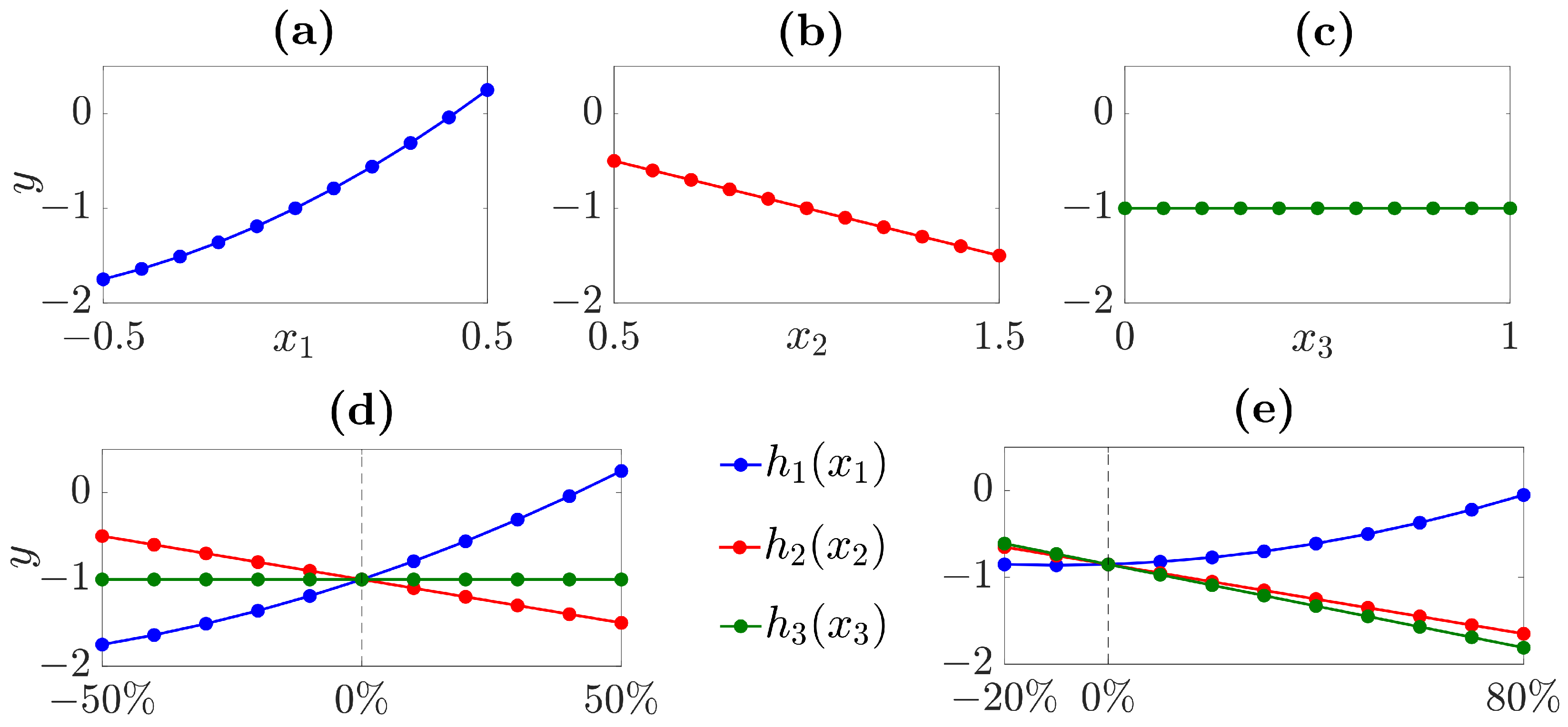
2.2.2. One-Way Sensitivity Analysis

As discussed in Section 2.2.1, insight provided by a Tornado diagram into the model sensitivity behavior is limited to specific OAT input perturbations (i.e., minimum and maximum values) with respect to the base case. Yet, for the analyst, it might be of interest to evaluate the model output at more than three points, so as to study the variation of the model output when each input, individually, varies inside its plausible range of variation. In this case, the so-called one-way SA may be used, which can be considered a generalization of the sensitivity measures provided by Tornado diagrams. The ease of implementation, intuitive nature, and effective result visualization make one-way SA one of the most popular SA methods in the power system field [75,76,77,78,79].
As for Tornado diagrams, in one-way SA, a base case x 0 , as well as plausible variation ranges for the inputs, x + = [ x 1 + , x 2 + , , x K + ] and x = [ x 1 , x 2 , , x K ] , shall be defined. The procedure starts with setting the inputs at their base case values except for input x i , which is left free to vary between its range extremes. The sequence of N points ( x i n , x i 0 ) , with n = 1 , 2 , N , is then considered, whereby x i is changed N times within its range of variation (producing the set of values { x i 1 , x i 2 , , x i N } ), while keeping all the other inputs fixed at their base case values ( x i 0 ). In particular, the first ( x i 1 ) and last ( x i N ) element of the sequence are the minimum ( x i ) and maximum ( x i + ) values of x i , respectively. The one-way sensitivity function h i ( x i ) can then be defined for input x i as:
h i ( x i ) = g ( x i , x i 0 )
After evaluating h i ( x i ) at the N different values of x i (with the other inputs held constant at x i 0 ), the model output values can be plotted against x i by performing some sort of interpolation, if needed. The procedure is then repeated for each of the remaining inputs. In total, the computational cost for running one-way SA of a model with K inputs equals N K model runs, where N is the number of values arbitrarily selected for each input x i . In the case of models with a low degree of smoothness, a high value of N might be required to achieve a sufficiently accurate description of the input–output sensitivity relationship.
In our toy example, for the first input x 1 varying in [ 0.5 , 0.5 ] the one-way sensitivity function h 1 ( x 1 ) calculated at, say, N = 11 points leads to a sequence of 11 model output values:
g ( 0.5 , x 2 0 , x 3 0 ) , g ( 0.4 , x 2 0 , x 3 0 ) , , g ( 0.0 , x 2 0 , x 3 0 ) , , g ( 0.4 , x 2 0 , x 3 0 ) , g ( 0.5 , x 2 0 , x 3 0 )
These values are recorded and plotted against x 1 in Figure 3a. By repeating the procedure for the two remaining inputs, the graphs in Figure 3b (for x 2 ) and Figure 3c (for x 3 ) are produced. By looking at the three upper plots in Figure 3, the effect on y is (mildly) quadratic and monotonically increasing for x 1 , linearly decreasing for x 2 , and null for x 3 . Hence, similar to the Tornado diagram in Figure 2, x 3 seems to have no effect on the output.
To visualize the model sensitivity behavior in a more compact manner, the one-way sensitivity functions are sometimes plotted in the same graph, which is called a “spider plot” [69,80]. Since in many practical cases the model inputs may have different units and/or scales, the input variations in percentage terms (instead of their absolute values) are shown on the x-axis of the spider plot. In our toy example, the corresponding spider plot is represented in Figure 3d, with the model input ranges varying between ± 50 % around the base case. Clearly, the indication given by a spider plot (and, in general, by one-way SA) is twofold. First, insight is provided into the direction of change of the model output when each model input is, individually, moved across its variation range, while holding the others fixed at x 0 . Second, information regarding the magnitude of the effect on the model output due to individual input variations can be extracted: according to Figure 3d, x 1 causes the biggest change in y, followed by x 2 , with x 3 having no effect at all. Here, the same considerations presented for the Tornado diagram hold: one-way SA, being OAT, cannot detect and quantify interactions between inputs.
One further point bears consideration: one might wonder whether it would be possible, in this case, to extrapolate the results obtained at a local level (i.e., for the base case x 0 ) to infer about the model sensitivity behavior at a global scale. Such a generalization of the results is, unfortunately, rarely possible. To convince the reader about this statement, consider for the toy example the same inputs’ plausible ranges, but a different base case, e.g., x 0 = 0.3 , 0.7 , 0.2 , shifted 30% with respect to x 0 = 0 , 1 , 0.5 . A one-way SA run with the new base case x 0 leads to the spider plot of Figure 3e: a different situation is clearly displayed. Here, the analyst would conclude that x 3 has now gained importance in affecting, with its variation, the model output, and by taking into account the magnitude of the output variations on the y-axis, x 3 would even rank first in the list, followed by x 2 . Input x 1 is now relegated to the last position, whereas in Figure 3d (considering the original base case x 0 ), it was responsible for the highest output variation. This intuitive proof shows how one-way SA might be highly dependent on the chosen baseline/operational point, and except for very particular cases (e.g., linear and additive models), the drawn conclusions are restricted only to the (small) investigated input space portion. Such a “location dependence” property is an intrinsic feature of local sensitivity measures, which, if used to infer the model sensitivity behavior at a global level, might lead to misleading conclusions. One might argue that this is not a desirable property to have for a sensitivity measure. However, this does not necessarily mean that local/OAT SA methods are to be discarded a priori, but, rather, the analyst shall be always aware of the outcome applicability range and accurately verify the model linearity degree in the case the extrapolation of the results is of interest.
To summarize, one-way SA is a straightforward and intuitive method whose informativeness about the model sensitivity is limited to OAT variations of the model inputs over their predetermined ranges while holding all the others fixed at the investigated base case. Being local and OAT, one-way SA does not provide the analyst with a thorough exploration of the whole input space, nor is it able to account for interactions among inputs, and it might be inaccurate unless some particular conditions (e.g., model linearity) are reasonably met. If the model properties are not known a priori or the underlying model linearity assumptions are too unrealistic to hold for the problem at hand, results derived locally are in general not necessarily informative at a global scale: extreme care should be taken in drawing conclusions elsewhere.

2.2.3. Scenario Analysis

Scenario analysis, a type of analysis often encountered in decision theory and economics (see, e.g., [81]), studies the model behavior at particular “scenarios”, i.e., a set of plausible (non-redundant) assumptions that aim at representing specific input configurations or possible future system states of interest [82]. In scenario analysis, as opposed to Tornado diagrams and one-way SA, inputs may be varied simultaneously to capture particular input changes and investigate specific input space locations. Although being a quite practical and decision-oriented SA method, scenario analysis has the downside of being highly subject to the discretion adopted by the analyst when selecting the scenarios to investigate. Moreover, only a small set of input configurations is generally considered. Power system applications (e.g., [44,79,83]) usually select scenarios so as to reflect particular high-stress grid configurations (e.g., the worst-case “generation peak and load valley” daily scenario), as well as to forecast some future network evolution (e.g., foreseen electric vehicle penetration, electricity demand or emission prices). Moreover, the so-called Scalability and Replicability Analysis (SRA) often adopts scenario analysis to evaluate the future potential of promising smart grid implementations and identify economic/regulatory barriers [84].
In its simplest form, scenario analysis starts with the scenario generation step, where a (generally restricted) set of alternative scenarios of interest is defined [85]. For example, commonly investigated scenarios are:
  • The “baseline” scenario, with all the model inputs kept at their base case values to study a reference situation;
  • The “worst-case” scenario, with all the model inputs set to values that reflect some unfavorable behavior of the model;
  • The “best-case” scenario, with all the model inputs set to values that produce a desirable configuration capturing some “well-behaved” pattern of the model.
A DoE method could be adopted as a strategy to assist the analyst during the scenario-generation step. For example, the so-called Taguchi orthogonal array testing [86] is occasionally adopted in power system applications to select a number of representative testing scenarios [87,88]. Obviously, alternative DoE strategies are available in the literature, of which a preliminary overview is offered in Chapter 2 of [9].
For our toy example, assume that the analyst—by resorting, e.g., to sector experts and practitioners, literature reviews, etc.—specifies the baseline, worst-case, and best-case scenarios to be x B a s e l i n e = 0 , 1 , 0.5 , x W o r s t = 0.2 , 1 , 0.8 , and x B e s t = 0.5 , 1.25 , 0.5 , respectively. By running a scenario analysis for the three selected scenarios, the model would lead to the values g ( x B a s e l i n e ) = 1 , g ( x W o r s t ) = 1.6 , and g ( x B e s t ) = 0 . It is noteworthy that x W o r s t and x B e s t need not be defined so as to coincide with the lower and upper endpoints (i.e., x , x + ), but as done here, combinations other than the extreme input values can reflect system states deemed by the analyst as worst- and best-case scenarios.
Clearly, with scenario analysis, the analyst can gain insight into the behavior that the model will have in the concerned scenarios also when more than one input at a time is changed simultaneously. However, it is not always immediate to map the model output variation to what is responsible for it. Strategies such as scenario decomposition [89] have been proposed in an attempt to circumvent this downside so as to obtain quantitative information about the causes of the variations observed in the model output.
To summarize, scenario analysis is an intuitively attractive SA method because it allows the analyst to study more complex model inputs’ changes than a simple OAT approach, yet generally focusing just on a restricted set of input configurations. Although being able to capture interactive effects between model inputs, scenario analysis does not provide a straightforward method to isolate the effect of such interactions (unless methodological extensions are considered) and is greatly dependent on the analyst’s subjectivity during the scenario generation step.

2.2.4. Differential Sensitivity Analysis

Differential SA is based on what can be historically considered as the first type of (local) sensitivity measure, i.e., the model output partial derivative. On the one hand, differential SA provides a very direct translation of the “sensitivity” notion; its computation is supported by a large family of efficient techniques (e.g., automatic differentiation, adjoint methods [90]), and it has been efficiently used in a variety of problem settings across disciplines (e.g., in power system applications dealing with optimization [91,92], system stability [93], reliability analysis [30], calibration [94], and, more generally, with large systems of differential equations). On the other hand differential SA is inherently local, finding its roots in the Taylor expansion of the model function at the base case x 0 . Consequently, the results of differential SA methods are in general applicable only in the close vicinity of the investigated input space portion around x 0 , and—unless the model is proven to be linear—they might be misleading if used to interpret the model behavior further away from the base case (intuitively, the farther the input perturbation is from the base case where the Taylor series has been built, the less accurate the results become).
In differential SA, the partial derivative of the model output (i.e., its rate of change) is computed with respect to each input x i at a specific base case x 0 . The resulting sensitivity measure for input x i is then:
S i = g ( x ) x i | x 0 i = 1 , 2 , , K
which measures the effect on the model output of perturbing x i around the base case x 0 = ( x 1 0 , x 2 0 , , x K 0 ) . S i can be easily approximated, e.g., via finite differences, i.e.:
S i = g ( x ) x i | x 0 g ( x 1 0 , x 2 0 , , x i 0 + Δ x i , , x K 0 ) g ( x 1 0 , x 2 0 , , x i 0 , , x K 0 ) Δ x i
In generic terms, the basic procedure for numerically estimating S i starts with specifying an ad hoc (arbitrarily small) size of the finite change Δ x i , which is generally the same for all the model inputs. Then, each model input is perturbed OAT by the given amount Δ x i around x 0 , the correspondent model output value is recorded, and the incremental ratio of Equation (7) is computed. Therefore, in its simplest form, differential SA would have a total computational cost of K + 1 model evaluations for computing S i . In practice, a high number of different algorithms exist for calculating S i , which efficiently implement numerical techniques based on finite differences, as well as automated differentiation [26,95].
In our toy example, S i (computed according to Equation (6)) assumes the following values for the three model inputs: S 1 = 2 x 1 0 + 4 x 3 0 , S 2 = 1 , and S 3 = 4 x 1 0 . As expected, S i is dependent on (and hence, sensitive to) x 0 . If two different base cases are considered, e.g., x 0 = 0 , 1 , 0.5 and x 0 = 0.3 , 0.7 , 0.2 as in Section 2.2.2, the resulting sets of the S i values would be, respectively, { S 1 = 2 , S 2 = 1 , S 3 = 0 } and { S 1 = 0.2 , S 2 = 1 , S 3 = 1.2 }, yielding two drastically different rankings for the three model inputs, similar to the Tornado diagram and one-way SA. This confirms what was already highlighted for local SA methods: unless the model itself is linear, the results derived from local sensitivity measures may be (even significantly) dependent on the input space location and are therefore informative only about a small neighborhood around the investigated nominal/operational point. By keeping this in mind, differential SA can nonetheless be useful for extracting twofold insight at a local level. In fact, not only can S i provide information about the direction of change—a positive (negative) sign of S i signalizes an increase (decrease) in the model output upon a small individual change of x i —but also regarding the relative significance of the model inputs—the higher the absolute value of S i , the bigger the influence of x i is. However, this latter inference on the model input importance can be made only if all model inputs have the same unit; otherwise, the absolute values of S i cannot be compared. To circumvent this scale limitation, it is common practice to introduce a normalization factor for S i so as to make the results commensurable (e.g., [96]). Frequently adopted weights are the input–output base case values (i.e., x i 0 g ( x i 0 ) ) or the input–output standard deviations (i.e., σ x i σ y ). In this latter case, the associated differential sensitivity measure becomes:
S i σ = g ( x ) x i | x 0 σ x i σ y i = 1 , 2 , , K
where σ x i reflects some known or reasonably hypothesized variability of the input x i and σ y could come from an earlier UA (e.g., via a Monte Carlo simulation). S i σ measures the effect on the model output of perturbing x i by a fixed fraction of the standard deviation of x i . In the power system field, S i and S i σ (or other normalized versions of S i ) are often referred to as “absolute” and “relative” sensitivity, respectively (see, e.g., [97]). It is noteworthy that the adoption of S i σ as a sensitivity measure—unlike S i —requires the analyst to make an assumption about the model input variation range for deriving the standard deviation values σ x i and σ y . As a consequence, although remaining formally “local” due to the presence of derivatives computed at a specific input space location, S i σ can be considered as a hybrid “local–global” measure, since information about the whole range of variation of the model inputs enters the sensitivity measure definition [28]. Normalized differential sensitivity measures such as S i σ should be hence preferred to S i for extracting information regarding the model sensitivity at a global level: in fact, by taking into account information about the input variability, in general, they allow for a more consistent model input global ranking, as opposed to absolute sensitivity measures such as S i [9].
To summarize, differential SA based on model output partial derivatives (i.e., S i ) has proven to be worthy in a wide set of applications (e.g., optimization, calibration, and inverse problems). Moreover, being supported by numerical techniques that complement simulation programs to efficiently compute large arrays of system derivatives (e.g., automatic differentiation and adjoint methods), differential SA may be particularly useful for large-dimensional and computationally expensive models, for which more sophisticated probabilistic SA methods might become less convenient. However, when resorting to differential SA, the analyst should be beware of the underlying local SA assumptions, which limit the applicability field. In fact, although extensions would be in principle possible (e.g., refining the analysis accuracy by considering higher-order partial derivatives to account for the interactive effects of multiple inputs), in general, differential sensitivity measures are informative—in terms of magnitude and the sign of model output change—only for small perturbations around the base case, unless the model is proven to be linear. Problems may arise—in terms of misleading conclusions—if results coming from these small perturbations (for which S i -based differential SA is intended) are used to make inferences at a “global” scale, in the presence of finite ranges of uncertainties. To this purpose, the hybrid local–global sensitivity measure S i σ offers a more consistent model input ranking, but its effectiveness diminishes as the model nonlinearity degree increases. In general, when large uncertainties are present in the inputs, the investigation of the whole input space is of interest, and the model has an unknown linearity degree (or it is known to contain nonlinear effects), differential SA offers just a limited view of the model sensitivity.
Simplicity, intuitiveness, inexpensiveness, and implementation straightforwardness are some of the main strengths of the local SA methods addressed in this section, making them undoubtedly attractive for studying the sensitivity behavior of the model at hand. However, as previously discussed, local SA methods study the model behavior only around single input space locations, and generally, no interactions among model inputs can be detected and quantified (even if some extensions might be adopted, such as higher-order derivatives or scenario decomposition). Overall, as noted in [98], the results deriving from a local SA should be always communicated along with the disclaimer that they are valid only at the given base case and when changing the inputs OAT. Hence, these methods may be unwarranted (or even inappropriate) to assess the relative importance of the model inputs in the presence of finite uncertainties when the model is nonlinear to a certain extent and/or no a priori information regarding the model properties is available. In these cases, global SA methods are in general recommended, which are reviewed in the next section.

2.3. Global Sensitivity Analysis Methods

Unlike local SA, global SA is performed by taking into account a probabilistic framework, with the specification of a PDF for the model inputs, which thus become random variables X i . When the analyst’s interest is not limited to a specific input space location, global SA should be preferred to effectively account for the whole model inputs’ uncertainty, being able to efficiently deal with large-dimensional systems, model nonlinearities, as well as different scales and degrees of input uncertainty. This section presents an overview of four global SA methods: the Morris method, correlation analysis, regression analysis, and variance-based SA.

2.3.1. Morris Method

The Morris (or elementary effects) method can be considered as an extension of the local approaches described in Section 2.2. Under the sampling strategy viewpoint, it belongs to the class of OAT designs, since it performs OAT variations of the model inputs. However, it partially overcomes the deficiencies of local SA methods in that it aggregates multiple OAT designs performed at random locations so as to remove any location dependence. For this reason, the Morris method can be classified as “global”: by allowing for a deeper investigation of the input space, it can hence track model nonlinearities and interactions. Given its computational inexpensiveness, this method is—especially for high-dimensional models—particularly well suited as a “screening” technique, i.e., for identifying (with a small number of model runs) non-influential model inputs that could be neglected in later analyses. This feature finds immediate applications, e.g., in the context of model dimensionality reduction [99,100] and can serve as basis for narrowing down the number of model inputs on which more informative (though more demanding) SA techniques can focus in a later step [101,102].
The fundamental idea of the Morris method, as originally developed in [103], aims at classifying the model inputs into three groups: (1) inputs whose effect is negligible; (2) inputs with linear and additive effects, not involved in interactions; (3) inputs involved in interactions or whose effect is nonlinear. This categorization is achieved by computing the so-called “elementary effects”. The elementary effect of input X i for a given perturbation Δ is the following incremental ratio:
E E i = g ( x 1 , , x i 1 , x i + Δ , x i + 1 , x K ) g ( x 1 , , x i 1 , x i , x i + 1 , x K ) Δ
The basic procedure of the Morris method starts by dividing the variation range of each input X i into p equally spaced intervals or “levels”—the value of p being chosen ad hoc by the analyst. The K-dimensional input space (a cube in our toy example, since K = 3 ) is therefore discretized into a p-level grid of points. The perturbation parameter Δ is then selected, such that Δ is a multiple of 1 p 1 . Moreover, a random point x r * from the p-level grid is chosen as a base point and used as the “seed” for generating the r-th “trajectory”, i.e., a sequence of points in the input space obtained from x r * by increasing or decreasing one or more of its K components by the same (randomly chosen) amount Δ . In particular, the first trajectory point x r ( 1 ) is obtained by varying one or more components of x r * by Δ , with the constraint that the shifted point x r ( 1 ) does not exit the p-level grid. The second trajectory point x r ( 2 ) is obtained from x r ( 1 ) , keeping all its components fixed except for the i-th component, which is increased or decreased by Δ (with the index i chosen randomly in the set { 1 , 2 , , K } of the inputs’ indices). The third trajectory point x r ( 3 ) is obtained by imposing that x r ( 3 ) differs from x r ( 2 ) for only one component j by the same amount Δ (for any j i ). This procedure is continued until the last trajectory point x r ( K + 1 ) is generated. The r-th trajectory so obtained consists of K + 1 design points (with the seed point x r * not being part of it) and can be used to compute one elementary effect per input, E E i r , with i = 1 , 2 , , K , by using Equation (9). The whole procedure is then repeated R times (each time randomly selecting the base point x r * ), thus generating R different trajectories that explore the input space in multiple locations. An example of R = 4 random trajectories is shown in Figure 4a.
Once R elementary effects per input are obtained ( E E i r , with r = 1 , 2 , , R ), their mean μ ^ i can be computed as follows:
μ ^ i = 1 R r = 1 R E E i r
Intuitively, μ ^ i evaluates the overall influence of input X i on the output, such that a high value (either positive or negative) indicates that X i is important. However, a low μ ^ i does not necessarily indicate an unimportant model input. In fact, μ ^ i (being based on the mean) is vulnerable to Type II errors, i.e., identifying an important input as non-influential. This can happen, e.g., for an input whose effects have alternate signs (canceling each other out): in these cases, the elementary effects would have an average close to zero although singularly assuming significantly high (positive or negative) values. To circumvent this limitation, an alternative sensitivity measure μ ^ i * is introduced [104], which computes the mean of the elementary effects in absolute value:
μ ^ i * = 1 R r = 1 R | E E i r |
Now, by using μ ^ i * , the magnitude of the input effect can be effectively assessed (low values of μ ^ i * unequivocally indicating low importance of X i ), but the information regarding the sign of the effects due to the input changes is lost. Therefore, the recommended practice is to compute both μ ^ i and μ ^ i * , so that their combined comparison can efficiently inform about both the magnitude and sign of the inputs’ effects on the model.
In addition to μ ^ i and μ ^ i * , also the variance σ ^ i 2 of the R elementary effects of input X i is a useful sensitivity measure and can be computed as follows:
σ ^ i 2 = 1 R 1 r = 1 R E E i r μ ^ i 2
By using σ ^ i 2 , the presence of nonlinearities and/or interactions in the model structure can be qualitatively detected. Intuitively, if σ ^ i 2 is small, the elementary effects of X i on the model output are almost the same everywhere, and the hypothesis of linearity in the relationship between Y and X i is likely to be true (a perfectly linear relationship would in fact yield σ ^ i 2 = 0 ). On the other hand, high values of σ ^ i 2 suggest that X i has on Y an effect that is nonlinear and/or due to interactions with at least one other input (although discriminating between either types of effects is not possible).
Since each trajectory is generated by moving only one input at a time, the Morris method is essentially based on an OAT design, but the R different OAT designs (i.e., the R trajectories) at different locations make the method way more informative than a pure OAT SA method. Other designs (e.g., [103,104]) have been proposed to take into account economy and efficiency considerations, yet the basic form of the method—as explained above—has a total computational cost of R ( K + 1 ) model runs. It is noteworthy that the efficiency of the Morris method is strictly related to the design choice; the selection of suitable values of p, Δ and R is thus a critical step. A convenient choice is usually to select p even and Δ = p 2 ( p 1 ) so as to guarantee an equal probability of selection of all the p levels. Previous works have proven that valuable results are produced by using p = 4 and R = 10 [105,106].
In our toy example, by considering p = 4 levels, Δ = 2 3 and R = 10 trajectories, the values of μ ^ i , μ ^ i * , and σ ^ i 2 are estimated and visualized in the so-called Morris plots, i.e., two separate planes ( μ ^ i , σ ^ i ) and ( μ ^ i * , σ ^ i ) , as shown in Figure 4b,c, respectively (where σ ^ i = σ ^ i 2 ) . By looking at the two Morris plots, the following conclusions can be extracted. Since none of the inputs is located close to the origin of the ( μ ^ i * , σ ^ i ) graph, all of them have an impact on the model output, included X 3 (whose importance, by adopting the earlier described local SA techniques, was quite ambiguous and mostly dependent on the investigated base case). Moreover, by looking at the ( μ ^ i * , σ ^ i ) Morris plot, X 2 is the least influential input (being closer to the origin of the graph than X 1 and X 3 ), whereas X 1 and X 3 seem to have comparable importance. Additionally, X 3 has the effects of alternate signs on Y (since μ ^ 3 0 and μ ^ 3 μ ^ 3 * ), whereas the effect of X 2 is linear ( σ ^ 2 0 ) and negative ( μ ^ 2 < 0 ). The high values of σ ^ 1 and σ ^ 3 further signalize that X 1 and X 3 are involved in interactions and/or their effect is nonlinear.
To summarize, via simple sensitivity measures such as μ ^ i , μ ^ i * and σ ^ i 2 and at a quite low computational cost, the Morris method can—qualitatively—provide insight into model structure (detecting the presence of nonlinearities and/or interactions) and input importance (in terms of the magnitude and direction of the effect). Due to its ability to scan the whole input space with a parsimonious number of points, the Morris method turns out to be particularly attractive as a screening technique, to identify noninfluential inputs and eliminate them from later stages of the analysis. Hence, it is a very convenient method for this purpose especially when the number of model inputs is high and/or the model computational time is too expensive for the analyst to adopt more sophisticated—and expensive—SA techniques (e.g., variance-based methods).

2.3.2. Correlation and Regression Analysis

Due to their strict conjunction with Monte Carlo simulation, methods based on correlation and regression analysis were among the first techniques to be developed and used for SA [107,108,109]. In general terms, correlation and regression analysis aim at retrieving information regarding output sensitivity through statistical post-processing of a Monte Carlo simulation. Although being simple and intuitive methods (often implemented in basic software packages of data analysis), their efficiency depends on the acceptability degree of the underlying assumptions (e.g., model linearity and/or monotonicity).
Before describing correlation and regression analyses, the procedure of a Monte Carlo simulation is briefly introduced. Monte Carlo simulation starts with building a sample matrix A, which contains a random sample of size NxK generated according to the inputs’ PDFs:
A = x 1 ( 1 ) x 2 ( 1 ) x K ( 1 ) x 1 ( 2 ) x 2 ( 2 ) x K ( 2 ) x 1 ( N 1 ) x 2 ( N 1 ) x K ( N 1 ) x 1 ( N ) x 2 ( N ) x K ( N )
In particular, the i-th column vector of the sample matrix contains N values of input X i (independently extracted from the input marginal PDF under the independence assumption among inputs), whereas each row vector represents a specific combination of the inputs’ values where the model can be evaluated. Although any random number generator can be adopted to produce the sample matrix, alternative sampling strategies exist that are often preferred due to their properties of input space filling and numerical efficiency, e.g., quasi-random sequences [110,111] or Latin Hypercube Sampling (LHS) [112].
By running the model with the different N input combinations of the sample matrix, the output vector y of the corresponding N Monte Carlo realizations is produced:
y = y ( 1 ) y ( 2 ) y ( N 1 ) y ( N )
Equation (13) (i.e., the sample matrix) together with Equation (14) (i.e., the collected model responses) constitute a basic Monte Carlo simulation of size N. A qualitative SA can be already performed by simply using such an input/output sample via the so-called scatter plots, which are often adopted to visually and qualitatively investigate the relationship between each input X i and the output Y [109,113]. In Figure 5, scatter plots for a Monte Carlo simulation of size N = 500 are generated for our toy example by projecting in turn the N values of the three inputs against the corresponding N Monte Carlo realizations. From the visual inspection of Figure 5, some insight into the model behavior can be already gained, e.g., the clear (though different) patterns in the distribution of points are indicators of some model output dependence on all the model inputs ( X 3 included).
Scatter plots are customarily used just as a preliminary or complementary step of a broader and quantitative SA study, including, e.g., correlation and regression analyses, which are described hereafter.
As regards correlation analysis, the simplest correlation-based sensitivity measure is the Pearson’s linear product moment correlation coefficient ( P E A R i ), which is based on the study of the correlation between the input X i ( i = 1 , 2 , , K ) and the output Y. In formal terms:
P E A R i = C o v ( Y , X i ) σ X i σ Y = n = 1 N x i ( n ) μ ^ X i y ( n ) μ ^ Y n = 1 N x i ( n ) μ ^ X i 2 n = 1 N y ( n ) μ ^ Y 2
where μ ^ X i and μ ^ Y are the sample means of x i ( 1 ) , x i ( 2 ) , , x i ( N ) and y ( 1 ) , y ( 2 ) , , y ( N ) , respectively, whereas C o v ( Y , X i ) is the covariance between X i and Y. The Pearson’s correlation coefficient can be seen as a linearity measure since it measures the strength of the linearity existing between X i and Y. It assumes values between −1 (in the case of a perfectly linear negative relationship) and +1 (in the case of a perfectly linear positive relationship), whereas it is equal to 0 if X i and Y are linearly independent.
In our toy example, the Pearson’s correlation coefficients (associated with the scatter plots in Figure 5) assume the following values for the three model inputs: P E A R 1 0.8 , P E A R 2 0.4 , P E A R 3 0 , meaning that the model output greatly depends on X 1 , followed by X 2 , with X 3 having almost null linear dependency on Y. In terms of the sign of change, it can be inferred that Y is positively correlated with X 1 (i.e., Y increases as X 1 increases), negatively correlated with X 2 (i.e., Y decreases as X 1 increases), whereas the null value of P E A R 3 indicates the absence of linear correlation between X 3 and Y, although the existence of a different well-defined nonlinear relationship cannot be excluded.
Connected to correlation analysis is regression analysis, which consists of building a regression model for the input/output sample coming from a Monte Carlo simulation. In the simplest form, assuming that the input/output mapping g ( · ) can be approximated via a linear relationship, the resulting linear regression model assumes the following form:
g ( x ) = b 0 + i = 1 K b i x i
where the regression coefficients b i s are estimated, e.g., by an ordinary least squares procedure. The value of b i characterizes the effect that a unit change in input X i has on the output. Since the b i s are generally dimensioned, it is common practice in regression analysis to adopt their normalized version as a sensitivity measure, i.e., the so-called “Standardized Regression Coefficients” ( S R C s):
S R C i = b i σ x i σ y
The values of S R C i , i = 1 , 2 , , K provide in general a better characterization of model input importance than their raw versions, since they incorporate information regarding the distribution assigned to the inputs. In particular, the S R C is related to the effect of perturbing each model input away from its expected value by a fixed fraction of its standard deviation (holding all other inputs at their expected values). In our toy example, S R C i P E A R i with i = 1 , 2 , 3 : it can be inferred, e.g., that the effect of perturbing the expected value of X 1 by a fixed fraction of its standard deviation is, in magnitude, almost twice the impact of X 2 .
It is noteworthy that, since the S R C (as defined according to Equation (17)) relies on the model linearity assumption, its “robustness” as a sensitivity measure is dependent on how well Equation (16) is an effective regression model for the Monte Carlo input/output sample. A measure of the accuracy of the regression fit is given by the coefficient of model determination R Y 2 :
R Y 2 = n = 1 N y ^ ( n ) μ ^ Y n = 1 N y ( n ) μ ^ Y R Y 2 [ 0 , 1 ]
where y ^ ( n ) is the model output n-th prediction obtained by using the linear regression model of Equation (16). In particular, R Y 2 represents the share of model output variance explained by the regression model and can be therefore interpreted as the fraction of linearity of the model: it is equal to one for linear models, whereas a small value signalizes a poor linear regression fit. Consequently, the robustness of the S R C s as sensitivity measures is conditional to the value of R Y 2 : values of R Y 2 , e.g., higher than 0.7 , might be considered acceptable to evaluate the relative importance of the model inputs based on the S R C s, but with the side-effect of remaining “ignorant” about the residual fraction of the model output variance [28]. In our toy example R Y 2 = 0.78 , meaning that we can still use the S R C s as sensitivity measures, though at the price of gaining no insight into more than one-fifth of the total output variance.
In many situations, the linearity assumption of the input/output relationship does not hold, hence leading to small values of R Y 2 . If the input/output relationship is nonlinear, but monotonic, the downsides associated with poor linear regression fits may be sometimes avoided via rank transformations [107,114], according to which the original samples are replaced with their corresponding ranks and, then, the usual regression is performed on the rank-transformed samples. In practice, the smallest value of x i ( i = 1 , 2 , , K ) is assigned a rank of 1, the next largest value a rank of 2, and so on, up to the largest value of x i , which is assigned a rank of N (equal to the size of the Monte Carlo simulation). With the same approach, the model output vector y is also rank transformed, and the rank-transformed versions of P E A R and S R C can be computed directly on the rank-transformed samples ( x i R and y R ). In particular, the rank-transformed versions of Equations (15) and (17) lead, respectively, to the Spearman correlation coefficient S P E A R [115] (an indicator of the monotonicity of the input/output relationship) and the Standardized Rank Regression Coefficient S R R C [107]. However, if on the one hand, rank transformations may be useful to convert a nonlinear, but monotonic input/output relationship into a linear one (with possible improvement of the regression fit in terms of higher R Y 2 ), on the other hand, the results derived from the regression of the rank-transformed model are generally not directly applicable to the original (non-transformed) model.
To summarize, SA based on correlation or regression analysis can lead to robust sensitivity measures ( P E A R and S R C ) if the underlying linearity assumption of the input/output relationship is reasonably verified. If the regression fit is poor (i.e., a low value of R Y 2 ), their performance might worsen. A partial circumvention to this limitation can be usually achieved with rank transformations, which may provide better linear regression fits in the case of nonlinear, though monotonic input/output relationships. Nonetheless, the rank transformation approach leads to the problem of mapping the conclusions coming from the rank model version back to the original model, and in general, it fails in the presence of multimodality in the model [116]. To disengage the analyst from any heavy reliance on prior assumptions regarding the model form (i.e., Equation (16) or its rank-transformed version) turning to model-free global SA methods should be considered: variance-based SA techniques are of this kind and are presented next.

2.3.3. Variance-Based Sensitivity Analysis

All the SA methods illustrated so far have been revealed to be applicable (and hence reliable) only under specific assumptions, generally telling just a part of the story. For example, local SA techniques are suited for studying the effect on the output of small changes in the inputs at a specific input space location, but are inappropriate when used far away from the base case (unless the model is linear) and fail in detecting and quantifying interactions between inputs. On the other hand, correlation and regression analyses—being based on Monte Carlo simulation—are revealed to be more complete to study the global model sensitivity behavior since they include a sort of multidimensional averaging over the whole input space and directly incorporate input distribution information, yet being able to explain the whole input variability only if specific model properties are verified (linearity/monotonicity). Methods based on the decomposition of the model output variance, falling into the category of the so-called “variance-based SA”, are able to overcome these limitations and reflect all four desirable SA properties mentioned in Section 1.1.6. Hence, if the analyst deems the variance as a satisfactory descriptor of model output uncertainty, variance-based SA is the suggested choice to make model-based robust inferences under uncertainty.
Variance-based SA methods have been widely considered as the “gold standard” for testing the input uncertainty effects in the model and have currently been consolidated as best practice inside the SA field, though still constantly facing massive developments [63]. Despite their recognized potential, variance-based SA methods have been underused in many research fields, though experiencing an encouraging increased attention in recent years (e.g., [39,59,60,61,117] for power system applications). The whole framework of variance-based SA methods was laid out in the early 90s [118,119,120], when the so-called Sobol indices were first introduced, although the idea of using importance measures based on the input contribution to the output variance dates back to the correlation ratio [121]. The underlying intuition behind variance-based Sobol sensitivity indices is given hereafter, whereas for further mathematical details, the reader is referred to, e.g., [9,118,122,123,124].
Consider the generic model Y = g ( X 1 , X 2 , , X K ) of Equation (1) —where the inputs X 1 , X 2 , , X K are independent random variables with a known PDF—and the research question “How much the model output Y is sensitive to the uncertainty in X i ?”. One possible approach to tackle this problem would be to assess how much the variance of the model output, V a r ( Y ) , decreases when fixing X i at its “true” value x i * . Intuitively, after eliminating one potential source of output uncertainty, the resulting conditional variance would be smaller than the original total variance, i.e., V a r X i ( Y | X i = x i * ) < V a r ( Y ) , where V a r X i ( Y | X i = x i * ) is the output variance taken over “all-inputs-but-i” ( X i ), conditioned to having fixed X i at a specific value x i * . Clearly, the “true” value x i * is not known, and a reasonable choice is thus taking the average of the conditional variance over all possible values of X i while all other inputs are left to vary, i.e., E X i ( V a r X i ( Y | X i = x i * ) ) . Given the law of total variance:
E X i ( V a r i ( Y | X i ) ) + V a r X i ( E X i ( Y | X i ) ) = V a r ( Y )
it follows that E X i ( V a r X i ( Y | X i ) ) V a r ( Y ) and V a r X i ( E X i ( Y | X i ) ) can be interpreted as the expected reduction of the output variance that would be obtained if X i could be fixed at its “true” value, whereas, intuitively, E X i ( V a r X i ( Y | X i ) ) is the residual output variance. According to this approach, if V a r X i ( E X i ( Y | X i ) ) is high, X i is an important input in conditioning V ( Y ) , and consequently, V a r X i ( E X i ( Y | X i ) ) can be used as a sensitivity measure. In particular, by a simple normalization, the so-called first-order Sobol index S i of input X i is obtained:
S i = V a r X i ( E X i ( Y | X i ) ) V a r ( Y ) S i [ 0 , 1 ]
The sensitivity measure S i provides the answer to the question: “What output variance reduction would be expected if uncertainty in X i is eliminated?”. In the SA framework, this “purpose” is called input prioritization “setting”, whose ultimate goal is to produce a ranking of the model inputs X 1 , X 2 , , X K based on their relative contribution to the output uncertainty. Under this setting, S i can be defined as the fraction of the model output variance that is due to X i alone or, equivalently, as the direct effect that X i individually has on the output uncertainty. Such information would be undoubtedly remarkable to identify relevant model inputs, e.g., for a successive calibration/optimization activity, as well as for prioritizing future research efforts aiming at reducing the output uncertainty (e.g., to identify the inputs deserving more “dedicated” measurements before actually starting to collect measurements for any of them).
However, if a high value of S i signalizes that X i is an important input, conversely, S i close to zero is not a sufficient condition for ruling X i out of the set of influential inputs: Equation (20) implies in fact that S i is blind at model interactions, which might, however, play a role. In other words, one model input might have no effect “at the first order” (i.e., it does not affect the output variability per se), but it might have an influence in combination with other model inputs. Hence, higher-order Sobol indices (that reflect higher order interactions between model inputs) can be built analogously to Equation (20). For example, the second-order Sobol index S i j of two inputs X i and X j quantifies the output variance fractional contribution due to the joint effect of the pair { X i , X j } after removing their first-order effects ( S i and S j ). Sensitivity indices of higher orders can be analogously defined up to the K-th interaction order. Provided that all the interaction terms can be computed, variance-based SA supplies an effective theoretical framework with which a full discernment of the model sensitivity behavior, as well as its inner structure could be gained. In fact, it can be demonstrated that, for a model with K inputs, Sobol indices are tied to each other by the following relationship:
i S i + i i < j S i j + + S i j K = 1
which can be seen as a (normalized) decomposition of the model output variance. However, the variance decomposition in Equation (21) (certainly appealing from a theoretical perspective) may suffer from the “curse of dimensionality”: since all the decomposition terms are as many as 2 K 1 , their computation might quickly become unfeasible and prohibitively expensive already for a relatively low number of model inputs. For a model with, say, 10 inputs, a full variance decomposition will require calculating already 1023 terms—undoubtedly an inconvenient and presumably unnecessary computational effort, as suggested by Pareto’s law (according to which it is likely to have often only a small subset of the input uncertainties responsible for most of the output uncertainty, mainly in terms of main effects and low-order interactions). To investigate higher-order effects though eluding this potential computational burden, the so-called total-order Sobol index T i of input X i is introduced [125]:
T i = E X i ( V a r X i ( Y | X i ) ) V a r ( Y ) = 1 V a r X i ( E X i ( Y | X i ) ) V a r ( Y )
where V a r X i ( E X i ( Y | X i ) ) represents the variance reduction that would be obtained, on average, if all-inputs-but- X i could be determined and fixed at their “true” values, whereas E X i ( V a r X i ( Y | X i ) ) represents the residual output variance. Under a reversed perspective, the latter quantity turns out to be nothing but the contribution to the output variance due to all terms of any order—in the decomposition formula of Equation (21)—that include X i . Hence, T i accounts for the overall contribution of input X i , including not only its first-order effect, but also all the other (higher-order) effects deriving from possible interactions with other inputs. For example, for a three-dimensional model, T 1 = S 1 + S 12 + S 13 + S 123 . Although the total order indices could be computed by calculating all the respective terms (e.g., S 1 , S 12 , S 13 , S 123 for T 1 ), strategies are available for their direct estimation, hence efficiently coping with the “curse of dimensionality”. It is worth noting that the set of all the first-order indices S i s along with all the total order indices T i s provides the analyst with a quite comprehensive (and parsimonious) picture of the global model sensitivity behavior: higher-order Sobol indices may be selectively computed only if the given model properties (e.g., interactions among specific pairs of inputs) should be further deepened.
The sensitivity measure T i is linked to the so-called input fixing setting, which provides the answer to the question: “Which model inputs could be fixed anywhere in their variation range without significantly affecting the output variance?”. In this setting, the ultimate goal is to detect non-influential model inputs that neither alone nor in synergy with other inputs have a substantial effect on the output variability. Such information would be significant, e.g., for confirming or confuting some prior belief of the analyst regarding the relevance of specific model inputs [126] and for model simplification (especially for complex and high-dimensional systems). In particular, T i 0 provides a necessary and sufficient condition for X i to be irrelevant in affecting the output variance. Inputs with almost zero values of T i are inconsequential and need not be better determined or modeled: they can be therefore “frozen” to any convenient value within their variation range (without appreciable loss of information for the model) and possibly discarded from a subsequent analysis. In fact, once the set of non-influential inputs has been determined, the complementary set contains only inputs that explain almost the whole output variance. Considerations of the approximation error due to such model simplification were discussed in [127]. It is noteworthy that T i has similarities with μ ^ i * (i.e., the sensitivity measure of the Morris’ method introduced in Section 2.3.1): either measures produce similar or even equal inputs’ rankings [104]. Hence, μ ^ i * is a good proxy of T i , and—although not having quantitative interpretation in terms of model output variance—it can be adopted for the input fixing setting: this is especially useful for high-dimensional, over-parametrized, and/or computationally demanding models, for which variance-based SA might become expensive.
Another setting worth mentioning is the so-called variance cutting setting, especially relevant when SA is used, e.g., in the context of risk assessment and management problems. According to this setting, a predefined reduction in the output variance V ( Y ) is to be achieved—e.g., below a given threshold V t h r ( Y ) —and an informed choice has to be made of which and how many model inputs should be better determined so as to maximize the success probability of obtaining V ( Y ) < V t h r ( Y ) (often with the requirement to simultaneously fix the least number of inputs). Such an analysis goal can be guided by the combined evaluation of S i s and T i s (and, if needed, also of higher-order indices), as described, e.g., in [124].
Variance-based sensitivity indices possess the following properties:
  • 0 S i T i 1 if the model inputs are independent;
  • i K S i 1 if the model inputs are independent;
  • i K S i = 1 if the model is additive (i.e., without interactions);
  • T i S i measures how much X i is involved in interactions with other inputs;
  • 1 i K S i indicates the overall amount of interactions among inputs.
In our toy example, the values of the Sobol sensitivity indices—for the moment, postponing computational considerations—are reported in Table 2, based on which the following conclusions can be extracted. The values of S i suggest that X 1 is the right candidate to bet on under the input prioritization setting: the greatest reduction in the output variability (up to 64% of V ( Y ) ) would be obtained if X 1 could be fixed to its “true” value. In other words, assuming that the “true” values of all uncertain model inputs may be “discovered” at the same cost through more measurements, resources should be thus allocated to obtain a better definition of X 1 (e.g., by dedicated experiments). To further exemplify, imagine that, after collecting more measurements, the “new” PDF of X 1 (from the original U 0.5 , 0.5 ) has become U 0.3 , 0.3 . If a new Monte Carlo simulation is run (considering this new uncertainty of X 1 ), a 54 % decrease in the estimated V ( Y ) can be observed. If instead, one had launched a measurement campaign to better determine X 2 and decrease its uncertainty by the same proportion (i.e., from U 0.5 , 1.5 to U 0.7 , 1.3 ), only a 10 % reduction in V ( Y ) would have been observed. This intuitively demonstrates how S i can be practically employed to obtain information regarding how to prioritize future research efforts within a resource-saving context: the output uncertainty can be reduced the most by “acting” primarily on the uncertainty of the most important inputs. Additionally, the only non-zero higher-order Sobol index is S 13 , thus recovering the suspected effect of X 3 “at the second order”: the uncertainty of X 3 does have an impact on the output variability, but only as a combined effect with X 1 . It is noteworthy that in this case, higher-order indices could be deduced directly from S i s and T i s: since S 2 = T 2 , it follows that S 12 , S 23 and S 123 are identically null and, consequently, S 13 is simply T 3 S 3 or, equivalently, T 1 S 1 . This shows that computing just S i and T i might be often sufficient for retrieving a satisfactory (or, occasionally, even complete) description of the model sensitivity behavior. Moreover, it is worth noting that, via the Sobol indices, not only the “real” effect of X 3 can be detected and quantified (i.e., 20 % of the output variance is due to the combined effect of X 3 and X 1 ), but also insight into the model structure can be gained (i.e., the presence of an interactive X 1 , X 3 term along with two individual effects of X 1 and X 2 ): such information was not accessible via any of the previous SA methods, hence vindicating the adoption of variance-based SA to achieve a full accounting of model inputs’ uncertainty. Furthermore, the non-zero values of T i suggest that—under the input fixing setting—none of the model inputs is inconsequential: all inputs, with their variation, do have an impact either individually (e.g., X 1 , X 2 ) or via interactive effects (e.g., X 3 ). Lastly, it is worth noting that the values of S i and T i produce two different rankings for the inputs, according to the different meaning of input “importance” conveyed by the two sensitivity measures under the input prioritization and input fixing setting, respectively.
Strictly speaking, the calculation of the Sobol indices would theoretically require computing conditional variances—e.g., V a r X i ( E X i ( Y | X i ) —which are nothing but multidimensional integrals in the input space. If the input/output mapping g ( · ) is a known and relatively easy function, Sobol indices may even be computed in closed form (as done for the indices of our toy example in Table 2). Alternatively, the multidimensional integrals required for computing Sobol indices could be estimated numerically [128]. Yet, to avoid this potentially cumbersome approach, shortcuts have been developed for estimating Sobol indices based on Monte Carlo simulation: one possible formula to estimate S i and T i is presented hereafter for the sake of illustration.
The procedure starts with generating a sample matrix Q of dimension Nx 2 K (where N is the size of the Monte Carlo simulation and K is the number of inputs) and dividing it into two submatrices of size NxK: the first submatrix (A) contains the columns of Q from 1 to K whereas the second submatrix (B) contains the columns from K + 1 to 2 K :
Q = x 1 ( 1 ) x i ( 1 ) x K ( 1 ) x 1 ( 2 ) x i ( 2 ) x K ( 2 ) x 1 ( N 1 ) x i ( N 1 ) x K ( N 1 ) x 1 ( N ) x i ( N ) x K ( N ) A x K + 1 ( 1 ) x K + i ( 1 ) x 2 K ( 1 ) x K + 1 ( 2 ) x K + i ( 2 ) x 2 K ( 2 ) x K + 1 ( N 1 ) x K + i ( N 1 ) x 2 K ( N 1 ) x K + 1 ( N ) x K + i ( N ) x 2 K ( N ) B
As many as K matrices A B i , i = 1 , 2 , , K are then generated such that A B i is composed of all columns from A except for its i-th column, which is taken from B:
A B i = x 1 ( 1 ) x K + i ( 1 ) x K ( 1 ) x 1 ( 2 ) x K + i ( 2 ) x K ( 2 ) x 1 ( N 1 ) x K + i ( N 1 ) x K ( N 1 ) x 1 ( N ) x K + i ( N ) x K ( N ) i = 1 , 2 , , K
Each row of the generated K + 2 matrices represents a given coordinate in the input space, since it contains a specific combination of input values. The model output is then computed for all the N ( K + 2 ) coordinates of each of the matrices A, B, and A B i , i = 1 , 2 , , K , generating the N-dimensional output vectors g ( A ) , g ( B ) and g ( A B i ) , respectively. The sample mean E ^ ( Y ) and variance V a r ^ ( Y ) of the output Y may be estimated by combining g ( A ) and g ( B ) as follows:
E ^ ( Y ) = 1 2 N n = 1 N g ( A ) ( n ) + g ( B ) ( n )
V a r ^ ( Y ) = 1 2 N 1 n = 1 N g ( A ) ( n ) E ^ ( Y ) 2 + g ( B ) ( n ) E ^ ( Y ) 2
where, e.g., g ( A ) ( n ) denotes the output value computed by evaluating the model function Y = g ( X ) at the n-th coordinate of matrix A. An analogous meaning holds for g ( B ) ( n ) and g ( A B i ) ( n ) .
To estimate S i , the quantity V a r ^ i = V a r X i ( E X i ( Y | X i ) ) , i.e., the numerator in Equation (20), may be computed by using model output values coming from coordinates of the matrices A, B, and A B i [122,129]:
V a r ^ i = 1 N n = 1 N g ( B ) ( n ) g ( A B i ) ( n ) g ( A ) ( n )
and S i is then obtained by dividing Equation (25) by the sample variance V a r ^ ( Y ) .
Similarly, to estimate T i the quantity V a r ^ T i = E X i ( V a r X i ( Y | X i ) ) , i.e., the numerator in Equation (22), may be computed by using model outputs associated with coordinates of matrices A and A B i [130]:
V a r ^ T i = 1 2 N n = 1 N g ( A ) ( n ) g ( A B i ) ( n ) 2
and T i is then obtained by dividing Equation (26) by the sample variance V a r ^ ( Y ) .
Error estimates for the Sobol indices can be obtained via various methods, e.g., asymptotic formulas [131] or bootstrap methods [132,133], which can be adopted for deriving confidence intervals and monitoring the convergence of the indices according to the accuracy required for the specific application.
Regarding the generation of matrix Q (leading to the two sampling matrices A and B), various strategies may be employed. Common practice is using “low discrepancy” sequences—also known as “quasi-random” numbers [110]—which are often preferred for their space-filling properties, being designed to cover the input space as uniformly as possible. In fact, especially for small N, a sampling strategy based on random numbers showcases areas in the input space where the function values are not sampled (“gaps”), as well as regions where they tend to be overemphasized (“clusters”). On the other hand, quasi-random sequences (e.g., the Sobol LP τ sequences [134]) tend to maintain an even spread of points throughout the input space, leading to enhanced numerical convergence rates, hence being particularly useful for the estimation of Sobol indices [111].
As regards the computational cost, the full set of S i s and T i s can be obtained at the price of N ( K + 2 ) model runs (with N usually varying between a few hundreds to one thousand), which might sometimes represent a limitation in case large-dimensional models should be investigated. In fact, if a single model run takes a significant amount of time (e.g., in the order of seconds or minutes), the computational time to achieve a reasonably accurate level of the estimation accuracy can become impractical. This major drawback has been often used as the main argument in disfavor of the applicability of variance-based methods. However, alternative techniques to circumvent the applicability problem for time-consuming models have been proposed, including spectral approaches (e.g., the Fourier amplitude sensitivity test [123] and its extended version [135], the random balance design [136,137], and the EASI method [138]) and metamodel-based methods [139] (e.g., by using Polynomial Chaos Expansion (PCE) [140,141] or Gaussian processes [142]). In particular, the latter class of methods is based on the so-called surrogate modeling, i.e., the process of building an “emulator” of the original simulation model. The emulator (or “metamodel”) is a model that mimics the behavior of the original potentially complex model (i.e., the relationship g ( · ) between Y and X 1 , X 2 , , X K ) via an easy-to-evaluate function, hence being more tractable and simpler than the original model [143]. Surrogate modeling finds application within SA in that a metamodel, after being fit to the input/output sample, can be used to estimate the sensitivity indices via simple post-processing, hence greatly decreasing the computational burden for their computation. Besides spectral and metamodel-based approaches, further possibilities especially useful for large-dimensional and time-consuming models include deploying grouped designs (where the same Sobol indices are computed for clusters of inputs), as well as preliminary screening techniques (e.g., Morris’ method) to selectively perform variance-based SA only on the restricted set of influential inputs.
Apart from computational considerations, a further potential drawback of variance-based indices is their implicit dependence on assuming variance to be a good “proxy” of output uncertainty. In fact, some circumstances might call for a different measure of output uncertainty: for example, if a specific range of the output PDF is of interest (e.g., its tails) or the output PDF shows some level of multi-modality and/or skewness, variance might not be the preferred option for fully describing output variability. In these cases, “moment-independent” sensitivity measures could be adopted, such as the entropy-based [144] and the δ [145,146] importance measures. In a nutshell, these sensitivity measures take into account directly the whole output PDF (by somehow assessing the divergence between conditional and unconditional output PDF) without resorting to any specific statistical moment of the output PDF (e.g., the variance).
Lastly, a consideration has to be made regarding the existence of possible correlations between model inputs. Inputs’ independence is a quite general assumption on which many SA methods rest (not only variance-based ones), not just because generating dependent input samples is less straightforward, but also due to some methodological and interpretative difficulties that might arise. However, it is widely recognized that neglecting correlation effects in the modeling activity may distort the SA results, and hence, caution has to be taken when dealing with the presence of dependence or correlation structures between inputs. For example, remaining in the context of variance-based SA, the variance decomposition formula of Equation (21) holds only when the inputs are independent; otherwise, counterintuitive results may appear (e.g., T i < S i for a negative correlation). When the input independence assumption is not valid and working with correlated model inputs cannot be avoided (e.g., by treating the input dependency as a noisy term [9]), technical modifications/extensions have to be taken into account, e.g., [147,148,149,150,151,152]. Alternatively, other approaches could be considered that do not rely on inputs’ independence assumptions, e.g., [144,145,153]. Nonetheless, SA with correlated inputs is an ongoing vivid research topic.
To summarize, variance-based SA allows the analyst to make informed choices under uncertainty by properly acknowledging all known sources of uncertainty (including interactive effects) and ensuring against the danger of neglecting influential inputs. The ability to reflect the model structure, the easiness of interpretation, and the model-free nature elect variance-based SA as a powerful and flexible tool to support the decision-making and modeling process under uncertainty, supplying reliable sensitivity measures also in the case of nonlinear models or, more generally, when information on the model properties is not available a priori. Notwithstanding the undoubted merits over local SA methods, the possible pitfalls of variance-based sensitivity measures might be the nontrivial computational cost and the reliance on model inputs’ independence assumption, but complementary or alternative methodological formulations are available to efficiently circumvent these possible downsides.
Variance-based methods are clearly not the only global SA techniques existing in the SA literature. Other possible global SA approaches are, e.g., derivative-based global sensitivity methods [154], density-based methods [145,155,156], entropy-based measures [144,157], and variogram-based methods [158,159]. Moreover, graphical methods exist that may be equally useful not only as fully fledged SA techniques (such as scatter plots [109], Contribution to the Sample Mean (CSM) [160] and Variance (CSV) [161] plots, CUSUNORO plots [162], and cobweb plots [163])—ultimately providing complementary or additional information to the selected SA method—but also as supporting visualization tools (e.g., radial convergence diagrams [164] and heat maps [165]).

3. Status Quo of Sensitivity Analysis in the Power System Community

Recent review papers produced by the SA community (e.g., [15,166,167,168]) have shown the tremendous advances accomplished by SA over the past years from both theoretical and application viewpoints. Yet SA—as a field of science on its own—still experiences significant misinterpretations, challenges and inappropriate practices when utilized as modeling support tool in many research branches [7]. This section aims at describing the status quo of SA within the power system field and can be considered as a “spin-off” of the literature analysis conducted in [6], where an extensive cross-disciplinary bibliometric study was carried out to review the SA state-of-the-art in the scientific modeling community. The main findings of [6] are summarized as follows.
  • A growing interest in the scientific community towards SA is observed in the recent years.
  • The majority of published SAs tends to adopt local and OAT approaches, often relying on unjustified assumptions regarding the linearity degree of the model hence undermining the analysis credibility.
  • A conceptual misunderstanding exists that leads to conflating the meaning of “sensitivity analysis” and “uncertainty analysis”, ultimately causing a degradation of the analysis quality.
  • Spread practice is to perform a global UA (e.g., by Monte Carlo simulation) alongside with a local SA.
  • Disciplines often based on large computer models (such as earth, environmental or energy sciences) surprisingly showcase rather low rates of global SA approaches.
The literature review presented in this section not only investigates the validity of these findings in the power system field but also highlights specific peculiarities and common practices to describe the SA state-of-the-art in the power system community. Hereafter the adopted approach for the literature review carried out in the present paper is described (Section 3.1 and Section 3.2) and its main outcomes are discussed (Section 3.3 and Section 3.4).

3.1. Strategy for the Bibliometric Study

In this work the literature review was performed by using the IEEE Xplore® digital library (available online at https://ieeexplore.ieee.org, accessed on 25 October 2021). The search criteria were intended to include an as wide as possible sample of papers so to enhance the bibliometric study significance and therefore the robustness of the review findings. In particular, the strings “sensitivity analysis” and “uncertainty” were set as mandatory in all paper metadata (i.e., title, abstract or keyword), whereas various strings broadly related to the modeling of power systems (e.g., “electrical network”/“power system”/“electrical grid”/“smart grid” and “model”/“algorithm”/“method”/“simulation”) were required to be present in the paper main body text. The adopted search specification is considered to be a reasonable choice for confidently focusing the attention on papers that claimed to perform some type of SA under uncertainty by adopting or developing models or algorithms specifically in the power system field. Nevertheless, despite the attempt of adopting as much general and neutral search specifications as possible, the sample of investigated papers is inevitably smaller than the actual number of papers adopting some kind of SA in power system applications.
The paper selection procedure has not been restricted to a specific period of publication time, thus returning articles ranging from 1981 to 2021. For the sake of representativeness, both journal and conference papers have been selected as target of the query specification. In fact, after an explorative search it has been noticed that, over the recent years, SA—and particularly global SA—has been increasingly adopted also in some conference papers, which have been then retained to give them due credit. Moreover, no minimum citation rate has been used as filter so to avoid any kind of bias in terms of paper publication date (since older articles are more likely to be highly-cited than the most recent ones).

3.2. Review Criteria of the Bibliometric Study

Each publication has been analyzed according to the review criteria described as follows.

3.2.1. Presence of Uncertainty and/or Sensitivity Analysis

Since the terms “uncertainty analysis” and “sensitivity analysis” are sometimes conflated [6], first of all it has been investigated whether any of these two analyses have been performed in the reviewed publications considering Definitions 1 and 2. According to these two definitions, UA aims at characterizing the output variability given the uncertainty in the model inputs (e.g., by estimating the output PDF and/or extracting summary statistics), whereas SA goes one step further and aims at apportioning the variability of the model output to its sources of uncertainty, investigating which model inputs, and to what extent, mostly drive the model output uncertainty.

3.2.2. Local/Global Sensitivity Analysis

The reviewed publications have been categorized according to whether SA has been performed following a local or global approach as described in Section 1.1.4. In particular,
  • in local SA the model output uncertainty is studied in terms of variation of the model inputs around a specific baseline (e.g., Tornado diagram, one-way SA and differential SA) or by focusing just on a restricted set of model inputs’ combinations (e.g., scenario analysis);
  • in global SA the model output uncertainty is studied by exploring the whole space of variability of the model inputs via OAT designs (e.g., in the Morris method) or AAT designs (e.g., in regression/correlation analysis, variance-based SA), without focusing only in a small neighborhood around a given nominal/operational point.

3.2.3. Method of Sensitivity Analysis

The reviewed publications performing SA have been investigated according to the adopted SA method. Since the focus of this literature review is on SA, no categorization of UA methods has been performed. An overview of UA techniques for power system applications can be found, e.g., in [169].

3.2.4. Paper Focus

The reviewed publications have been analyzed according to the context for which SA has been used, dividing them between model-focused and method-focused papers.
  • In model-focused papers the main concern of the publication is a specific algorithm/model, with SA serving purely as a support tool for evaluating the model sensitivity behavior under uncertainty. In this case the paper outcomes are application-oriented, i.e., mainly related to the model rather than to the SA method.
  • In method-focused papers a specific SA method is introduced, developed or tested under various perspectives (e.g., numerical convergence, computational cost, scalability, etc.), whereas a model/algorithm is used only for the purpose of testing the SA method, whose performance is the main focus of the paper.

3.2.5. Model Type

As discussed in Section 2, when SA is inappropriately performed (e.g., adopting local and OAT methods to infer the relative importance of the model inputs in the presence of uncertainty in circumstances where the model linearity hypothesis is quite unrealistic or not valid), SA results might be inaccurate or could lead to even grossly misleading conclusions especially for nonlinear models [8]. In view of this consideration, the model investigated in the reviewed publications has been examined under the linearity degree viewpoint to assess the appropriateness of the SA performed on it. In particular the model type was classified as “linear” (if the model was distinctly linear or some linearized version was adopted), “nonlinear” (if some degree of nonlinearity was detected in the model itself, in the objective function or in its constraints) or “unclear” if no safe inference was deducible.

3.2.6. Software for Sensitivity Analysis

Numerous software packages have been developed over the recent years with the aim to operationalize and ultimately promote the usage of SA throughout the scientific community. In this regard, the software adopted to run SA in the reviewed publications has been hence recorded, where indicated. It is worth noting that most of the available SA computer packages specifically implement global SA routines, due to their undoubtedly higher implementation complexity with respect to local SA techniques (which, in their basic form, just require coding derivative-based algorithms or perturb-and-observe approaches).

3.3. Results of the Bibliometric Study

The literature search carried out in the IEEE Xplore® digital library resulted in 297 publications (both conference and journal papers). Approximately 9% of these has been discarded for different motivations, such as:
  • the paper content actually did not perform any UA or SA (according to Definitions 1 and 2);
  • the paper was the conference version of a journal article already reviewed (thus avoiding the presence of duplicates);
  • the topic of the paper was not related to the power system field.
Eventually, the sample of papers retained after this preliminary screening step consisted of 269 publications, simply referred to as “article pool” from now on.
According to the review criteria of Section 3.2, the article pool have been scrutinized by identifying the presence of UA/SA, the local/global approach adopted for running SA, the specific SA method, the paper focus, the model type and the software used for SA. Table 3 provides an overview of the results, which are discussed hereafter.

3.3.1. Presence of Uncertainty and/or Sensitivity Analysis

According to Table 3 the article pool consisted of 56% publications where UA has been performed, whereas in 44% of the cases UA was absent. This is not surprising since the adopted search specification is not required to match exactly the keyword “uncertainty analysis”, being the focus of the bibliometric study on SA. Although ideally UA and SA are run in tandem with UA preceding SA, there might be cases where this double step is not necessary and SA is immediately performed without first running UA. The subset of the article pool where UA is absent includes works related, e.g., to optimization problems [91,92], model parameter calibration [94], system stability [93], control [170] and operation [47].
Turning to SA, it has been carried out in 81% of the article pool, whereas in 19% of the cases the reviewed papers did not show any SA. In particular, in the latter group of papers no SA according to Definition 2 was carried out, but the analysis therein performed was rather an UA according to Definition 1. In other words, although the keyword “sensitivity analysis” was mentioned in the reviewed paper, the performed analysis aimed at characterizing the model output uncertainty (job of UA), without any attempt to somehow assess the relative contribution of the inputs’ uncertainty to the output variability (job of SA). This result is clearly an example of the “terminology problem” already pointed out in [6,7], according to which some authors perform an “uncertainty analysis” calling it instead “sensitivity analysis” (e.g., [171,172]) or use the two terms interchangeably (e.g., [173]).

3.3.2. Local/Global Sensitivity Analysis

According to Table 3 only 15% of the article pool adopted global approaches, whereas the majority of the SAs was based on local (mostly OAT) techniques (66%). For the sake of example, the following paragraph (taken from [52]) clearly indicates a local SA (in particular a one-way SA method): “the sensitivity analysis was carried out by evaluating the uncertainty contribution of each LV load power measurement on the estimated upstream power flow (UPF). In order to evaluate the uncertainty contribution of each LV measurement, UPF was evaluated considering the presence of only that measurement, assuming that in all the other nodes, the loads powers are known without uncertainty. In such a condition, the Monte Carlo analysis was carried out (105 iterations), randomly changing the considered power measurement within its uncertainty range. All the other LV measurements were kept constant at the values of the reference load condition”. On the other hand, the following sentence (taken from [58]) unequivocally refers to a global SA approach: “In this paper, variance-based sensitivity indexes are evaluated. The main idea is to decompose the variance of an output as a function of the main effects of each factor and possible interactions”.

3.3.3. Method of Sensitivity Analysis

Figure 6 reports the distribution of the SA methods described in Section 2 classified into local and global approaches. One-way SA is by far the most represented category of local SA methods (e.g., [75,76,77]). Differential SA is also quite common (e.g., [32,51,174,175]) and includes SA methods based on first as well as second order derivatives in both static and dynamic systems. SA based on scenario analysis (e.g., [44,79,83]) and Tornado diagrams (e.g., [70,71]) are less represented.
As regards global SA, variance-based methods are the most common technique, with the Sobol indices being computed via classical Monte Carlo direct estimation (e.g., [59]), spectral techniques (e.g., [102]) and metamodel-based approaches (e.g., [58,61]). Morris method is also quite adopted (e.g., [100,101]), whereas techniques based on correlation analysis (e.g., [176]) and regression analysis (e.g., [177]) are less represented. Global SA methods not reviewed in Section 2.3 are put into the same group (labeled as “Other” in Figure 6) and include, e.g., entropy- and density-based techniques (e.g., [178,179]).

3.3.4. Paper Focus

According to Table 3 a consistent slice of the article pool (79%) has its focus on the algorithm. This huge portion of application-oriented papers use SA as support tool, i.e., for studying the performance of their models/algorithms under various sources of uncertainty. In particular only 11% of the model-focused papers have adopted global SA methods, whereas the remaining part relies on local SA methods.
On the other hand, only 21% of the article pool was represented by method-focused papers, where SA methods have been proposed and tested on systems of various complexity. In 84% of the method-focused papers local approaches have been developed, often tailored to the application model for which they have been originally conceived. Examples of this category include, to name a few:
  • Ref. [41], where a fuzzy set theory based sensitivity index is developed in the context of reliability analysis of phasor measurement units;
  • Ref. [180], where a “wind curtailment sensitivity index” and the respective sensitivity matrix are developed in the context of transmission network congestion;
  • Ref. [52], where a strategy for optimal placement (in terms of number and location) of low voltage measurement devices is developed based on a “sensitivity order”;
  • Ref. [19], where an analytical methodology is presented for calculating a set of well-known reliability indices (e.g., loss of load probability, expected power not supplied, loss of load frequency) with respect to variations in equipment failure and repair rates;
  • Ref. [43], where a composite sensitivity factor based method is proposed in the context of distributed generation planning aggregating power loss and voltage sensitivity factors;
  • Ref. [46], where a second-order differential SA method is proposed for assessing the optimal solution sensitivity in the context of power systems with embedded power electronics;
  • Ref. [49], where a generator swing sensitivity index is proposed for evaluating the synchronous generator transient stability performance;
  • Refs. [33,34,35,36,37,181], where analytical formulas for voltage sensitivity analyses are derived ultimately for voltage regulation and control strategies in distribution networks;
  • Refs. [75,182], where different OAT sensitivity indices are calculated and tested on electrical machine systems.
On the other hand, only 16% of the method-focused papers proposed global SA techniques, such as:
  • Ref. [183], where three global sensitivity indices are proposed by combining principal component analysis and variance-based SA methods, considering correlated model inputs and multiple outputs for the study of microgrid operation;
  • Ref. [184], where “impact coefficients” of binary inputs are defined by establishing a model to decompose mean and standard deviations of grid node locational marginal prices in an ANOVA-like fashion [14,133,185];
  • Ref. [186], where techniques for modeling the stochastic correlation between model inputs are implemented and evaluated from their performance viewpoint in the context of power system small-disturbance stability;
  • Ref. [100], where a strategy based on the Morris method is applied for priority ranking of the model inputs whose correlation is modeled with the multivariate Gaussian copula method in the context of voltage and angular stability;
  • Ref. [187], where variance-based SA coupled with the Rosenblatt transformation [188] is proposed for correlated inputs in the context of voltage unbalance mitigation in active distribution grids;
  • Ref. [189], where a sequential experimental design based approach is used for building a surrogate model in the context of an all-electric warship AC/DC conversion system;
  • Refs. [39,176], where different global SA methods are tested in power system studies for input priority ranking.
From these results it is evident that, as expected, there is a wide predominance of papers that do not focus on the SA per se, but rather largely use SA as support tool. Local SA methods are widely adopted, whereas global SA methods are less frequently applied.

3.3.5. Model Type

According to Table 3 most of the papers (76%) adopted nonlinear models, whereas just a small portion (4%) was characterized by linear models or linearized versions. In 20% of the cases it was not possible to acknowledge the model linearity degree. From these results the tendency to work with nonlinear models (especially due to the complex behavior of power systems) seems evident.

3.3.6. Software for Sensitivity Analysis

For the reviewed publications the type of software package adopted for running SA has been recorded, where indicated. In particular, it seems to be widespread the usage of SimLab (e.g., [59,190,191,192])—no more available for download at the time of writing this review—and UQLab (e.g., [61,117,175]), whereas the usage of other software packages such as SAFE, SALib and SobolGSA appears to be less prevalent.
In order to provide the reader with a comprehensive—albeit not exhaustive—overview of software tools which are available to execute SA routines, Table 4 reports a list of computer packages for SA—not only those recorded in the article pool—with indication of the respective programming language and proper references. It is noteworthy that these packages reflect different design philosophies due to the diverse disciplinary background of the development teams and, beside local/global SA routines, include techniques also for other purposes such as uncertainty analysis, machine learning, reliability analysis, optimization, etc.

3.3.7. Trend of Sensitivity Analysis over Time

Figure 7 shows the time evolution of the SA papers reviewed in this bibliometric study by plotting the number of papers adopting local and global SA methods (from 1987 till 2021). According to Figure 7 there seems to be a clear generalized growth of SA papers in the last two decades. Notwithstanding a clear prevalence of local SA methods, an encouraging trend seems emerging in the last ten years to apply global SA approaches: it can be speculated that the first books entirely dedicated to SA ([9,11,12] dated 2000, 2004 and 2008, respectively) might have encouraged the spread of SA good practices.

3.4. Outcomes of the Bibliometric Study

Although the literature review performed in the present work clearly did not cover all papers performing SA in the power system field, the reviewed article pool can be considered as a quite representative sample for providing the reader with a reliable snapshot of the SA status quo within the power system community. The main findings derivable from the above results are presented hereafter. It is noteworthy that some of the outcomes largely confirm the findings of the cross-disciplinary study performed in [6,7]—being hence applicable to the whole modeling community since they reflect cross-disciplinary common trends—whereas other findings reflect discipline-dependent common practices encountered during this review work and are therefore assumed to be applicable specifically to the power system sector.

3.4.1. Increased Interest in Sensitivity Analysis

The number of research works performing SA during the modeling activity has been evidently growing in the last decade, revealing a raising interest of the power system community in the SA tool. SA has been adopted in applications such as power system robustness analysis [93], voltage control [32,33,34], voltage stability analysis [42], frequency support [38,39], network planning [43,44,204], generator [205] and load [206] ranking, reliability analysis [40,41], islanded microgrid loadability [179], dynamic response prediction [48], meter placement [52], energy storage capacity optimization [50,51], parameter calibration [94], network design [45] and reconfiguration [47]. Additionally, software tools developed for specific power system applications occasionally include built-in modules for performing SA (mostly adopting local SA methods). Some examples are [207] for power system optimization, [57] for distribution grid voltage management and [208] for transmission network risk assessment. Growing attention is also observed towards the relationship between SA and surrogate modeling: once a metamodel is created—e.g., via PCE [58,209,210], Gaussian Process [211] or Machine Learning [212]—it can be utilized in place of the original (potentially computationally demanding) model not only to perform time-consuming activities (e.g., probabilistic power flow [213,214], uncertainty [117,215] or tolerance [216] analysis) but also for running expensive SA techniques [61,217].

3.4.2. Prevalence of Local Sensitivity Analysis Methods

Local SA is more customarily employed as compared to global SA: as reported in Table 3 up to 66% of the article pool employed SA methods based on local approaches, even if in 76% of the cases nonlinear models have been studied/adopted. Under conservative assumptions—i.e., the models whose linearity degree was not assessable are hypothesized to be linear—this means that at least more than 2 5 of the reviewed papers have made use of methodologically poor and inadequate SA. Prevalence of local SA techniques is probably due the long tradition of linear SA approaches such as adjoint network method [53] (based on the application of Tellegen’s theorem), Jacobian method [55] (a byproduct of Newton–Raphson algorithm for solving power flow equations) and trajectory sensitivity (e.g., for studying small-signal stability in dynamic systems). Despite their demonstrated efficiency in many power system applications, these SA methods are primarily limited to first or second order approximations around operational or equilibrium conditions and, as already explained in Section 2, they cannot properly assess the influence of the full variation range of the uncertainty sources (e.g., large changes of power generation and consumption) as well as the effect of model nonlinearities: if the exploration of the whole input variability space is of interest and model linearity assumptions are too strong or unrealistic to hold—or even not communicated along with the results—local SA reveals to be inappropriate and insufficiently insightful, likely turning into a quite perfunctory activity [8]. Nonetheless in the last years a growing trend of papers adopting global SA has been recorded and establishment of small research groups focusing on global SA methods has been acknowledged.

3.4.3. Tendency to Perform Global Uncertainty Analysis Together with Local Sensitivity Analysis

When UA and SA are run in tandem, there is the quite widespread tendency to perform global UA (i.e., based on exploring the whole variability range of the inputs as for global SA) alongside with local SA methods. The prevalence of global approaches for performing UA (mainly via Monte Carlo simulations) is probably due to the long tradition of Monte Carlo based methods [218,219], which have been routinely adopted from the very beginning in power system applications [220,221]. More precisely, the tendency is observed to run quite huge Monte Carlo simulations (of size in the order of thousands of points per input) for estimating the output uncertainty, generally followed by one-way SA and spider plots to visualize the corresponding results. It is worth noting that in all these cases the chance is wasted to gain a deeper insight into the model sensitivity behavior via more quantitative SA techniques. More specifically, if the analyst’s mindset already encompasses the possibility to invest time and resources in consistent sample sizes, then the computation of, e.g., variance-based sensitivity indices would come at no additional cost ultimately leading to an increase of both informativeness and quality of the analysis.

3.4.4. Incorrect Beliefs Regarding Sensitivity Analysis

Beside the already mentioned terminology problem—according to which the meaning of UA and SA is sometimes conflated so that the analysis is stopped at the output uncertainty quantification stage without actually identifying the most relevant variability sources—some incorrect beliefs are occasionally encountered and are reported hereafter.
  • Although the need for SA as a diagnostic tool is properly acknowledged, it is sometimes believed that local methods are the only viable approaches for running SA (clearly ignoring the existence of global SA techniques).
  • Even if global SA is known, local SA is at times preferred to it and used under the specific motivation that the model at hand is “simple” and only a restricted amount of inputs are considered. In this regard, Section 2 has proved that even a not prohibitively complex model can conceal traps for the analyst and extreme care has to be taken when producing inferences by resorting to local and OAT SA methods. If the assumptions behind local and OAT SA methods are not valid, an uncertainty source locally not relevant might in fact reveal to be a key driver at a global scale or might gain importance because of its involvement in interactive effects with other inputs.
  • Common arguments sometimes used in disfavor of global (especially variance-based) SA are, e.g., the computational burden (when high-dimensional systems are to be studied) or the inability to capture specific model properties (e.g., the direction of change produced in the model output by the inputs’ variability): these beliefs ultimately motivate the preference for local and OAT SA methods. As already discussed in Section 2.3.3 the computational cost to estimate Sobol indices can be effectively decreased by adopting alternative possibilities such as metamodel-based techniques (e.g., via PCE [140]) or sequential approaches (e.g., first performing an initial SA via cheap screening methods and then adopting a quantitative method). On the other hand certain model features of interest such as the sign of the effect, the input/output relationship, etc. can be easily retrieved at no additional cost by integrating graphical methods in the global SA workflow (e.g., scatter plots [109], CSM [160] and CSV [161] plots, CUSUNORO plots [162], cobweb plots [163]).
  • When variance-based SA is used, the inputs’ ranking based on first order Sobol indices ( S i ) is sometimes expected to be consistent with that obtained according to the total order Sobol indices ( T i ): such expected agreement between rankings might signalize a conceptual misunderstanding supposedly related to unclear knowledge of the SA settings. As discussed in Section 2.3.3, S i and T i convey two different concepts of input “importance” and might assume different values for the same input, hence the two associated rankings need not to be necessarily identical. In particular, S i produces a ranking of the inputs according to their individual contribution to the output uncertainty, whereas T i considers the overall effect of a specific input both alone and in synergy with other inputs. Therefore, as exemplified in Table 2, an input with small or null S i (i.e., almost negligible under the input prioritization setting) might have a significantly higher value of T i hence acquiring not negligible importance (under the input fixing setting) given its involvement in interactive effects.

3.4.5. High Level Categorization of Power System Applications

As mentioned in Section 2.3.3 and further discussed in Section 4, the very first crucial step in SA is the definition of the “sensitivity question”: only by carefully formulating the objective of the analysis (or “setting”, according to SA terminology), the most suitable sensitivity measure can be identified and confidently adopted to answer the original question of concern [98,124]. Interestingly, most of the power system applications encountered in the reviewed publications can be categorized under different SA settings. For the sake of example, the input prioritization setting is directly connected, e.g., to performance analysis of state estimation algorithms [222] (e.g., to identify the measurements most influencing state estimation accuracy and suggest optimal meter placement), whereas the input fixing setting is related, e.g., to input screening [223], model dimensionality reduction [101,102] and priority ranking of critical components affecting system performance and stability [39]. As discussed in Section 2.3.3, the input prioritization setting could be effectively tackled, e.g., by resorting to the first order Sobol index, whereas, e.g., the total order Sobol index as well as the sensitivity measure μ ^ i * of the Morris method are appropriate measures for the input fixing setting.

4. Global Sensitivity Analysis at Work: Ready-to-Use Workflow with a Technical Example

This section provides a practical workflow that illustrates the recommended steps and the key aspects to consider for running global SA, together with exemplary conclusions, which can be inferred therefrom. A purposely simple technical example taken from basic electrical circuit theory was adopted to support (power system) user’s understanding of the methodology and dispel the possible fear that global SA is too complex to perform. The global SA methodology illustrated hereafter is general enough to be straightforwardly applied to more complex power system use cases for the study of the model sensitivity with respect to inputs affected by various types and degrees of uncertainty.

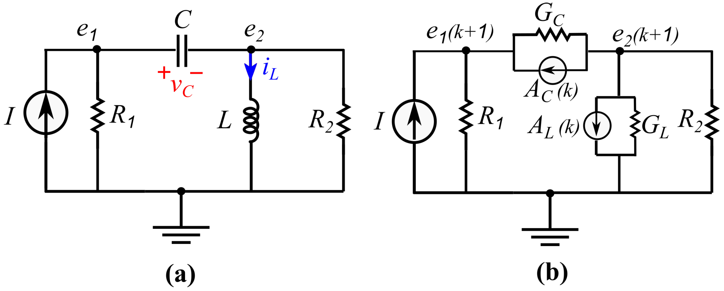
4.1. The System under Study

Figure 8a depicts the system under study, which is an elementary DC power system (potentially part of a larger one) made of a combination of resistors R 1 and R 2 , an inductor L, a capacitor C, and a current source I (for sheer simplicity, these capital letters are used for indifferently referring to both circuit elements and associated physical values). The voltages at the two circuit nodes are e 1 and e 2 ; the current flowing through the inductor is i L ; the voltage across the capacitor is v C . It was assumed that the exact values of the five circuit elements (I, R 1 , R 2 , L, C) are known with some degree of uncertainty, e.g., because of the tolerances of the design parameters by the manufacturer.

4.2. The Suggested Workflow

Figure 9 summarizes the suggested step-by-step workflow for running global SA. In the next sections, each step is first explained in generic terms, and its instantiation according to the system under study is then discussed.

4.2.1. Define the Analysis Purpose

The first (often overlooked) step of any SA exercise is accurately formulating the analysis purpose: a poor definition of the underlying objectives may in fact lead to unclear or ambiguous results. As previously seen, a variety of methods based on different assumptions and concepts of “importance” are theoretically available for running SA, but only a few of them are usually appropriate for the specific problem at hand. Hence, the overarching goals of the analysis shall be correctly defined beforehand so as to securely guide the analyst in the following choices: only a careful planning of the analysis ensures in fact that the answer to the original question can be confidently entrusted to a well-defined sensitivity measure [9].
In our system under study of Figure 8a, assume that the analyst is interested in determining the effects of the system variability sources (i.e., the uncertainties of the model inputs I, R 1 , R 2 , L, C) on the system state in terms of voltage (e.g., to ensure grid voltage stability) and/or current (e.g., to comply with line thermal constraints). Hence, the analyst may be confronted with the following questions:
  • Which of the system variability sources contributes to the system state uncertainty the most?
  • Do any of the system variability sources have a negligible impact on the system state uncertainty?
  • Does the model sensitivity behavior change over time?
  • Do certain modeling choices affect the system state uncertainty?
According to Question 1, the analyst aims at producing a ranking of the model inputs in terms of their relative contribution to the output uncertainty to prioritize future research efforts (e.g., discover the need for data quality improvement, allocate resources to gather—if possible—more measurements for subsequent input calibration, etc.). According to Question 2, the analyst’s goal is to detect possible noninfluential inputs, which, though affected by some variability, do not significantly impact the model output uncertainty and can hence be confidently ignored and removed from the model (e.g., for model simplification). According to Question 3, since the system state is time dependent, the analyst is interested in the time evolution of the sensitivity measures to gain insight into the system dynamics (which might be potentially unknown) and verify the model structure (i.e., checking that the model behavior is consistent with the modeler’s expectation). Lastly, according to Question 4, the analyst wants to assess if (and, in the case, to what extent) the system state uncertainty is dependent on discrete modeling assumptions (e.g., in terms of alternative model formulations, simulation time steps, etc.).

4.2.2. Identify the Model

After framing the questions that the analysis is expected to answer, the simulation model to adopt for the problem at hand has to be selected.
In our system under study, the selected model to perform transient simulation was the “resistive companion” approach [224], a classical method to solve dynamic circuits according to which each dynamic component (here, L and C) is transformed into a corresponding DC equivalent circuit, whose algebraic representation can be obtained via a specific numerical integration method (e.g., Euler backward, Euler forward, trapezoidal rule, Runge–Kutta, etc. [225]). By combining the individual resistive companion representations of all the circuit components, a system matrix relationship is obtained, which can be solved at each simulation time step until the end of the simulation time interval.

4.2.3. Identify the Model Output

Additionally, a decision has to be made about which model output to consider (also potentially varying in time or space) to reflect the analysis goals. Theoretically, many outputs could be selected to study the model behavior under different facets (hence leading to a multi-output SA [226,227]), and different levels of output aggregation and resolution may be considered according to the application of interest. For example, in the context of power system voltage stability, a summary statistics (e.g., the total number of times the voltage values at any node exceeds a given threshold over a specific time interval) is likely to be more practical and more informative for a stakeholder than considering the voltage values at all grid nodes (whose number might be also in the order of hundreds or thousands). Providing SA results for each grid node voltage, although theoretically feasible, would imply too many numbers to look at, probably making SA itself quite ineffective and out of scope. In other words, as all choices made by the user during SA, the selection of the output should be goal-oriented instead of model-oriented, i.e., focused on the answer the model is supposed to provide rather than on the model output itself [28]. Obviously, the consequent SA results are strictly dependent on (and “sensitive” to) the definition of the quantity of interest selected as the output.
In our system under study, imagine that the analyst is interested in voltage stability. Hence, among the various possible outputs produced by the model, v C (i.e., the voltage across the capacitor) is selected as the system state of interest to which the goals formulated in Questions 1–4 refer. Clearly, an application with an alternative focus would imply considering a different output, e.g., i L might be selected if the investigation of line thermal constraints would be of interest.

4.2.4. Identify the Model Inputs

The model inputs that might potentially affect the model output variability have to be properly identified and selected: for their definition, the analyst can benefit from participatory contributions by stakeholders, field experts, modelers, etc. [228]. As shown in Figure 1, the model inputs may be of various natures, e.g., measurement data, model parameters, alternative model structures/formulations, scenarios, boundary conditions, spatial/temporal resolution levels, etc. Importantly, SA can deal with model inputs that might be not only continuous (i.e., characterized by a continuous PDF), but also discrete, as in the case of categorical/qualitative attributes. The possibility to include discrete model inputs within SA is particularly important in the power system field since non-numerical inputs are often encountered (e.g., open/close switches, controllable/uncontrollable energy sources, ON/OFF status of home appliances, mesh and time step size of the simulation, time series, different load models, etc.). Additionally, all model elements not subject to SA (i.e., excluded from the model inputs’ set) have to be fixed at their baseline values. It is noteworthy that, since the analyst will remain clueless about the influence of all model elements that are excluded from the model inputs’ set, extreme care has to be taken during the inputs’ identification step due to its direct implications on the SA results and ultimately on the analyst’s capability to understand the model sensitivity behavior.
In our system under study, the following inputs were considered for SA: I, R 1 , R 2 , L, C. On the other hand, model elements not subject to SA were the integration time step, the numerical integration method, and the initial conditions at t = 0 for the circuit transient simulation. In particular, the trapezoidal rule was selected as the integration method (according to which the L and C elements of the original circuit (Figure 8a) are replaced by their DC-equivalent circuits, as in Figure 8b), with Δ t = 1 ms as the integration time step. This choice, without entering into mathematical details, was assumed to be a good compromise in terms of simulation accuracy, stability, and complexity. Moreover, the initial conditions for the circuit transient simulation were set to v C ( 0 ) = 0 V and i L ( 0 ) = 0 A.

4.2.5. Characterize Model Input Uncertainty

Once the model inputs subject to SA have been identified, their uncertainty has to be characterized: each model input is therefore assigned a PDF reflecting the analyst’s degree of knowledge about it. Various sources may be useful to extract the required information for characterizing input uncertainty, e.g., experts’ opinions, analyst’s experience, consultation of sector standards and the literature, knowledge from previous experiments, etc. In absence of specific information about the input PDF, it is customary to assume a uniform PDF (for which only the extreme values of the variation range are to be specified), whereas if more detailed knowledge is available (e.g., mean and variance of the input distribution), a Gaussian PDF would be usually the preferred choice. Of course, any other type of PDF could be adopted if specific information regarding the input distribution is obtainable. A correlation structure—e.g., in terms of a covariance matrix—might also be defined if appropriate. Intuitively, also this stage reveals to be crucial for the SA quality: in fact, since global SA methods rely on defining distributions for the model inputs, the SA results—and the corresponding conclusions—may be affected by alternative definitions of the known inputs’ uncertainties [229].
In our system under study, assume that the five selected model inputs (I, R 1 , R 2 , L, C) were considered independent (i.e., with identity covariance matrix) and their uncertainty was described by the PDFs reported in the third column of Table 5.

4.2.6. Choose the Method for Sensitivity Analysis

The selection of the fittest SA method for the problem at hand depends on considerations such as:
  • Purpose of the analysis—and potentially its final audience as well—in terms of the question the analyst is willing to answer (e.g., focus on a small neighborhood around an operational point or on the whole variability range, interest in input prioritization and/or model simplification, aim to understand the model structure, etc.);
  • Model computational cost (in terms of number of model evaluations the analyst can afford), dependent on the model execution time and number of model inputs (e.g., for high-dimensional and time-consuming models, a low-cost SA such as the Morris method is more suitable than variance-based techniques, which might be too expensive);
  • Prior model knowledge: if the model is very simple (e.g., linear and additive), local/OAT methods might be applied, whereas if the model properties are a priori unknown (e.g., in the case of “black box” models) or the model linearity assumption does not hold, global model-free methods (such as variance-based SA) are the recommended choice;
  • Presence of constraints on the inputs (e.g., correlations between them, multivariate distribution properties, etc.).
For a “getting started” guidance to select the most proper SA method for the problem under study, the reader can benefit from Section 2, which supplies an intuitive description of the methodological bases of the most widely used SA methods, with focus on their applicability boundaries, relative merits, and drawbacks. A more detailed “when-to-use-what” classification of a wider set of SA methods can be found, e.g., in [15], Chapter 31 of [10], and Chapter 6 of [9]. If different SA methods are available for the same problem, it is suggested to adopt more than one technique to perform a cross-comparison of the results and consolidate the drawn conclusions. This approach may often come at almost zero extra computational cost since many SA methods usually can be applied to the same input/output dataset with no need for additional model runs.
In our system under study, variance-based SA was selected due to the following considerations:
  • It can easily deal with all the goals stated in Questions 1–4;
  • Neither the computational time (8 ms for model run by using an Intel® CoreTM i5-7200U CPU laptop with 8 GB RAM), nor the number of model inputs (five) are, in this case, a limiting factor;
  • It does not rely on prior modeling assumptions (being model-free).
As regards the latter point, it is worth noting that the model function g ( · ) describing the system under study is known (e.g., in terms of state space model representation); nonetheless, it is assumed to be too difficult to treat analytically (as in more complex power system applications). Hence, model-free SA methods that do not require a priori any specific model knowledge (such as variance-based methods) are extremely useful and in general recommended.
As regards the computation of the Sobol indices, a PCE-based approach [140] is used instead of the traditional Monte-Carlo-based direct estimation to reach numerical convergence at a smaller sample size. It is worth noting that adopting a metamodel-based approach for estimating the sensitivity indices has the added value of equipping the analyst with an emulator that can be efficiently used in place of the original (potentially time-consuming) model also to carry out time-demanding tasks.
The required SA computations were performed by employing the UQLab software package [193] interfaced with our own codes in MATLAB® for simulating the power system under study of Figure 8.

4.2.7. Generate the Input Sample

After defining a PDF for each model input, the obtained K-dimensional input space Ω contains the whole information regarding the inputs’ properties in terms of variability range, distribution shape, correlation structures, etc. Drawing an input sample from Ω —as in Equation (13)—is hence the following step, for which two main aspects are to be considered: the sampling strategy and the sample size N.
The sampling strategy is mainly dependent on the chosen SA method: if the analyst has full control over the “positioning” of points in the input space, designs based on random and quasi-random numbers, as well as LHS designs are commonly adopted and are largely available in any SA software package.
The sample size N depends not only on the chosen SA method, but also on the model computational time, the latter normally being the limiting factor compared to the time needed to estimate the sensitivity measures. Generally, it is difficult to define beforehand the optimal sample size N for each SA method, it being the outcome of a (quite empirical) trade-off between computational cost and accuracy. Nonetheless, the common practice is to start with a small sample size N and progressively increase it until the desired level of accuracy in the sensitivity index estimates is reached (e.g., monitoring the estimate confidence intervals obtained via bootstrap techniques [132,133]).
In our system under study, the adopted sampling strategy was based on quasi-random Sobol LP τ sequences (although other low-discrepancy sequences could be used [110]). Convergence of the estimates of the Sobol indices (computed via the PCE-based approach) was reached at N = 64 , which was then chosen as the sample size.

4.2.8. Evaluate the Model

The generated input sample obtained from the specific design according to the selected SA method is then used for performing a Monte Carlo simulation. By evaluating the model at each specific combination of input values, the model responses are collected. If no computational model is available (e.g., in the case of field measurements or laboratory tests), the generated input sample matrix can still be seen as an experimental design, according to which each configuration of inputs’ values corresponds to one specific experiment to carry out.
In our system under study, the generated input sample (e.g., in the form of the input sample matrix in Equation (13)) is used to run the model from t = 0 ms to t = 40 ms with Δ t = 1 ms. The corresponding values of the model output v C are then collected for each time step.

4.2.9. Estimate Output Uncertainty

By generating the input sample with the desired properties (PDF, correlation structure, etc.) and performing a Monte Carlo simulation, the uncertainty of the inputs is propagated forward through the model all the way to the output. At this stage, the variability associated with the model output may be characterized and quantified with a UA, e.g., by extracting the output distribution and/or some summary statistics (such as mean, variance, median, percentiles, etc.).
In our system under study, the results coming from running a Monte Carlo simulation at each time step are reported in Figure 10a, where the evolution of v C over time is shown from t = 0 ms to t = 40 ms (one curve corresponding to one time-varying value of v C ). For each time step, the distribution of the values of v C can be extracted and represented with a histogram, as done in Figure 10b for three different time steps ( t = 1 ms, t = 2 ms, t = 10 ms). Histograms already allow inferring some output distribution properties, e.g., the variance of v C (the “spread” of its values over the horizontal axis) increases over time, and so does the mean. Additionally, quantitative insight into the output uncertainty can be gained by extracting specific descriptive measures of its distribution, such as the mean and standard deviation (e.g., μ = 21.5 V, σ = 12.0 V at t = 10 ms).

4.2.10. Extract the Sensitivity Measures and Interpret the Results

After being characterized, the output uncertainty can then be apportioned to all sources of variability or, in other words, mapped back to the model inputs so as to identify which of them are mainly responsible for the model output uncertainty and measure their impact. The input sample and the corresponding model output values previously produced are hence used to extract the sensitivity measures according to the selected SA method.
In our system under study, assume that the analyst is interested in assessing whether v C , given the uncertainty in the model inputs, stays within predetermined voltage limits when the steady state is reached at t = 40 ms. The distribution of the values of v c at this time is shown in Figure 10c. It can be seen that v C varies between 0 V and almost 80 V ( σ = 17.3 V at t = 40 ms); this variability is not acceptable for the analyst, who is hence willing to know where this uncertainty mainly comes from (Question 1) and if there are some noninfluential model inputs that can be excluded from the analysis (Question 2). To tackle these two problems, first- and total-order Sobol sensitivity indices are estimated, and their values are reported in Table 6. At the steady state, only I and R 1 have non-zero first- and total-order Sobol indices; a closer look at their values suggests the answers for Questions 1 and 2. In particular, most of the variance of v C ( 93 % ) is explained by the individual effects of I and R 1 (with S i = 0.31 and S i = 0.62 , respectively). If the analyst aims at reducing the variability of v C , resources should be allocated to better determine R 1 (whose uncertainty contributes to 62 % of the output variance). At the steady state, the other three inputs ( R 2 , L, C) have influence neither individually ( S i = 0 ), nor in combination with other model inputs ( T i = 0 ), signalizing that there would be no need to obtain a better determination and modeling of their uncertainty: R 2 , L, and C could hence be fixed to any given value within their variation range and discarded from a subsequent analysis. Moreover, the quantity T i S i for I and R 1 signalizes a slight interaction between them: it can be deduced, also without computing the second-order Sobol indices, that the interactive effect between I and R 1 contributes to 7 % of the output variance.
Table 6 describes the output sensitivity only at a specific simulation time ( t = 40 ms), thus representing a “sensitivity snapshot” of the system under study. However, the analyst might wonder whether the sensitivity behavior of the model changes over time, e.g., to check its internal consistency (Question 3): such an answer can be easily obtained by repeating SA for each time step of the simulation time interval. The obtained results are reported in Figure 11, where the time evolution of first-, total-, and second-order Sobol indices is presented. At the beginning of the simulation, the main contribution to the output variability is due to the uncertainty in I and C, whereas R 1 has a smaller proportional impact. As time goes on, C loses its importance (due to the capacitor discharge, as expected), whereas R 1 increases its effect until it becomes the dominant input, followed by I. On the other hand, the uncertainty of R 2 and L has an effect neither individually ( S i = 0 ), nor in combination with other inputs ( T i = 0 ). The time evolution of the total amount of model interactions can be also assessed with the quantity 1 i = 1 K S i , which is plotted in Figure 11c (dashed line): the model interactions reach a maximum around t = 6 ms (contributing to almost 10 % of the output variance), then decreasing until they stabilize. In particular, it can be seen that, at the steady state, the model interactions are entirely due to the second-order interactive effect among I and R 1 : S i j = 0.07 for the input pair { I , R 1 } , hence explaining 7 % of the total output variance.

4.2.11. Iterate Sensitivity Analysis (if Needed)

In general, SA is an iterative process: the conclusions drawn after a first SA run may in fact be used as feedback for the analyst to progressively refine the uncertainty of specific inputs (e.g., those spotted as the “most influential” ones), to guide during the model building process (e.g., by removing non-influential inputs, of which a more accurate modeling/determination would not be necessary), or to selectively investigate different model features (e.g., by adding new inputs or changing certain modeling assumptions). New iterations may also be required if the estimates of the sensitivity indices are not satisfactory under the robustness and convergence viewpoints: in this case, the sample size of the Monte Carlo simulation can be progressively increased, and SA can be repeated until the desired level of accuracy is met.
In our system under study, imagine that, after collecting the results of Table 6 and Figure 11, the analyst is interested in assessing whether specific structural modeling choices have an influence on the output uncertainty, as stated in Question 4. In particular, assume that a decision is to be made about which integration method to use among the trapezoidal rule and Euler backward (the former being more accurate than the latter, for the same time step). To include this aspect into the analysis, the original input set (I, R 1 , R 2 , L, C) is augmented with a sixth input ( M e t h o d ), which assumes only two discrete values (e.g., zero and one) that can be chosen with the same discrete probability [230]. Similar to a “Russian roulette” system, if the value zero is sampled, the system is solved with the trapezoidal rule; otherwise, Euler backward is adopted. By introducing this additional integer-valued input as the “trigger” among the two numerical integration methods, it is then possible to assess how sensitive the output is to the choice of adopting the two integration methods. After repeating the SA, e.g., at time t = 10 ms with all the inputs of Table 5 plus the inclusion of M e t h o d as an additional model input, the corresponding results are reported in Columns 2 and 3 of Table 7: R 1 and I almost equally contribute to the output variance, whereas only 4 % is due to C. Mild interactions emerge among R 1 , I, and C. Interestingly, the integration method choice ( M e t h o d ) does not contribute to the output uncertainty at all ( S i = T i = 0 ): this can be due to the fact that, although the trapezoidal rule is a more accurate integration method, the integration time step used for the simulation ( Δ t = 1 ms) is small enough to also let Euler backward produce accurate results. Hence, with Δ t = 1 ms, the analyst can indifferently choose among any of the two methods.
Another SA iteration might be performed to understand what happens if the integration time step is increased, e.g., from Δ t = 1 ms to Δ t = 10 ms. The SA results at t = 10 ms with Δ t = 10 ms are reported in Columns 4 and 5 of Table 7. Now, M e t h o d accounts for 10 % of the model output uncertainty ( S i = 0.10 ) and turns out to be even more important than a specific circuit element (C), meaning that one source of variability influencing the analysis is actually the integration method choice itself. In this case, the analyst should first decide which method to use (presumably the most accurate one), and once this variability source is fixed, the real sensitivity behavior of the output with respect only to the circuit elements’ uncertainties could finally emerge without any interference. Of course, other discrete inputs could be defined and similarly studied in an SA framework.

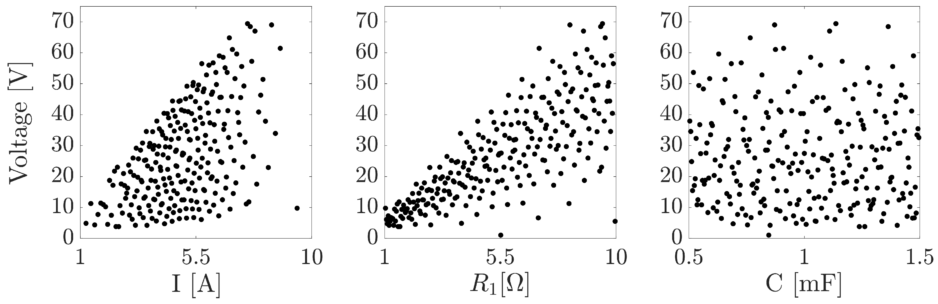
4.2.12. Complement Sensitivity Analysis with Graphical Tools

At the end of any SA activity, it might be useful to communicate results in an intuitive and easy-to-understand way, by keeping in mind both the purpose of the analysis and the scientific background of the SA final user. In this regard, graphical tools might be very helpful for effectively conveying the SA outcomes, especially when dealing with big sets of sensitivity indices. To this scope, a classical way is the use of a pie chart, where the whole model output variance is divided among the different sources of uncertainty (in terms of individual effects, as well as interactive effects). Additionally, a visualization of the input/output samples via scatter plots [109] or cobweb plots [163] can represent an effective complement of the information gained via SA. A detailed discussion of useful visualization and graphical tools for SA (outside the scope of this paper) was provided in [15,231].
In our system under study, the pie chart of Figure 12 provides a visualization of the different uncertainty sources that contribute to the total output variance at t = 40 ms: each slice represents, in percentage terms, the non-zero (first- and second-order) Sobol indices of Table 6.
The scatter plots in Figure 13 present a visualization of the individual effects of I, R 1 , and C on the output v C along their ranges of variation at t = 40 ms. Analysis of the scatter plots provides insight into the input/output relationship (e.g., type of trend, sign of the effect, etc.), hence representing a valuable complement to the information conveyed by the Sobol indices (which are scalar “condensed” sensitivity measures). For example, a well-defined pattern in the distribution of points signalizes high output sensitivity to the input (such as in the case of R 1 and I), whereas a rather uniform cloud of points is an indicator of small sensitivity (such as in the case of C).
As the scatter plots cannot capture possible interactions among the inputs, the cobweb plots can be adopted to efficiently visualize all the combinations of the inputs leading to a specific set of model output values (e.g., below or above a certain threshold). For example, the cobweb plot in Figure 14 highlights the input combinations leading to values of v C higher than 50 V at t = 40 ms; it can be immediately inferred that these specific input combinations (i.e., the black trajectories) specifically correspond to large values of both I and R 1 . In other words, I and R 1 are the influential inputs for producing output values falling inside the range of interest (i.e., v C > 50 V), whereas R 2 , L, and C are not relevant in this regard, since the black trajectories are distributed over their whole range of variation.

5. Operative Hints and Remarks for Sensitivity Analysis

Some concluding remarks and operative suggestions are presented hereafter.

5.1. No One-Fits-All Method

A single SA method does not exist for all problems at hand: the choice of which SA method to use is greatly influenced by considerations such as the model execution time, number of model inputs, prior knowledge regarding specific model properties (e.g., linearity, monotonicity, etc.), model accessibility (i.e., input samples already given or freely producible), and ultimately, the purpose of the analysis. This aspect does not constitute a drawback, but rather, it represents the real power of SA, which can be flexibly shaped and instantiated according to the specific application at hand. Moreover, combining multiple SA methods—which often come at no additional cost—might be helpful not only for a cross-comparison of the results, but also for exploring different research questions.

5.2. Appropriately Frame the Sensitivity Analysis Question

A proper SA starts long before becoming engaged with numbers and experiments: the foremost step is actually the activity of framing the SA question (the “setting”, using SA terminology), i.e., the formulation of the problem that the analysis is called to answer such that the appropriate sensitivity measure can be identified. An accurate definition of what is meant by “importance” can protect the analyst from producing misleading or poorly informative results, since generally, each sensitivity measure produces its own input ranking according to its corresponding concept of “importance”.

5.3. Mind the Assumptions of the Sensitivity Analysis Method

Before drawing any conclusion, it is essential to be aware of the SA method’s underlying assumptions, which consequently define the applicability boundaries of the method itself. No SA method is wrong per se: problems start appearing when an improper use of the SA technique is made, e.g., adopting local SA for inferring the model global sensitivity behavior in the presence of large uncertainty (unless the model is known or proven to be linear) or utilizing linear regression analysis for highly nonlinear models (i.e., with low values of R Y 2 ).

5.4. Investigate the Impact of Discrete Model Inputs

A typical feature of power systems is the widespread presence of uncertain model inputs that are discrete, such as categorical attributes (e.g., ON/OFF status of switches and energy sources), qualitative attributes (e.g., accuracy level of measurements), different time and/or spatial resolutions (e.g., size of the time step to use for numerical discretization schemes), alternative modeling choices (e.g., static or dynamic load models), etc. The study of the effect of these discrete model inputs—when not completely neglected—is often separate from that of the other (continuous) model inputs, i.e., multiple SAs are run by selecting, in turn, different values of the discrete model inputs. However, as shown in Section 4.2.11, discrete model inputs can also be straightforwardly incorporated into a single global SA activity by means of a “trigger” (used as a pointer to individual discrete inputs), so as to assess how sensitive the model output is to the choice of adopting alternative modeling choices in the presence of other uncertain model inputs. It is not uncommon, in fact, to observe that discrete modeling choices are as important as—or even more important than—“conventional” sources of uncertainties (e.g., model parameters, measurement errors, etc.). Moreover, the integration of discrete model inputs into the SA framework might inform the analyst about the acceptability degree of certain simplistic modeling choices. For example, it can be assessed whether the adoption of a simple ZIP load model would be a reasonable choice without the need to resort to more detailed composite load models or whether “convenient” (e.g., not significantly small) integration time steps could be employed for transient simulation without significantly impacting the model output uncertainty.

5.5. Integrate Sensitivity Analysis Routines into the Modeling Workflow

Some authors [6,27,63] have argued that potential obstacles hindering the widespread use of methodologically sound SA throughout the scientific community are a lack of technical skills (e.g., in statistics), the unavailability of resources (including time), and miscommunication among disciplines (e.g., between SA practitioners and SA final users), leading non-specialized analysts to often resort to very simple and intuitive (but sometimes inappropriate) SA methods. However, in recent years, there has been a huge effort in building easily accessible software tools (of which a comprehensive list is reported in Table 4) to support cross-disciplinary researchers with SA and ultimately promote its usage. These automatized SA routines—available in the most common programming languages—can be easily integrated into the user’s methodological workflow in a quite effortless fashion (i.e., just interfacing the modeler’s algorithm with the selected SA software package).

5.6. Perform Uncertainty Analysis and Global Sensitivity Analysis in Tandem and Iteratively, Wherever Meaningful

Given that many global SA methods are compatible with Monte Carlo simulations used for UA, global SA often comes at no extra cost; hence, running UA and global SA in tandem—unless for a few circumstances for which running a preliminary UA might not be needed, e.g., model calibration, optimization—is usually a recommended practice, in that it greatly deepens the analyst’s insight capability. Iterating the whole UA-SA activity is also beneficial, e.g., for a selective refinement of the inputs’ uncertainty and to perform an informed revision of the model definition.

5.7. Prefer Global Sensitivity Analysis Methods to Local and OAT Approaches in the Presence of the Inputs’ Uncertainty

If the model inputs are affected by finite uncertainties, only designs that are explorative of the whole input space (as those of global SA) are able to properly “shaken” the model to let its “inner substance” come to light. Hence, global SA methods should be in general preferred with respect to widespread local techniques (often relying on OAT designs), turning out to be inappropriate for efficiently investigating complex systems under uncertainty. In addition, global SA methods (such as variance-based techniques), which are also model-free, able to quantitatively assess interactions among model inputs and capable of treating groups of inputs, could dramatically enhance the analysis quality and—perhaps more importantly for the final user—provide an effective communication of the SA results, ultimately allowing for reliable inferences under uncertainty. To exemplify, quantitative and global conclusions such as “three of (the) fifteen inputs have (effect on) 88% of the total variance of the active power loss […] and the input P 671 (the active power injection at bus 671) should be considered first if one wants to reduce the active power loss (the most)” [61] would be clearly more informative than a qualitative and local deduction such as “when the uncertainty of the (wind generation) forecast increases, the total revenue of wind farms reduces” [232]. Note that the former statement derives from variance-based SA, whereas the latter represents the typical inference coming from one-way SA (adopted by the largest fraction of papers reviewed in this work as described in Section 3) and is valid only at the given base case and for OAT variations of the inputs.

5.8. Stimulate Participation in the Sensitivity Analysis Activity

Active participation of modelers, sector experts, stakeholders, and ultimately decision-makers into the whole SA process is an important aspect, in that it can fruitfully support the SA activity, e.g., during the identification of the model inputs to consider, the characterization of their uncertainty, the interpretation of the results, the actions to take for a further revision of the model, etc. This external contribution would invaluably augment the quality of the SA results, ultimately helping SA to become a successful activity.

5.9. Assess Sensitivity Analysis Robustness

The sensitivity measures of the adopted SA method (e.g., Sobol indices in variance-based SA, S R C s in regression analysis, etc.) might be uncertain themselves, being often estimates that are retrieved “empirically”, i.e., numerically obtained from the available input/output sample and not directly from the model equations. Consequently, assessing the accuracy of the sensitivity measures (e.g., in terms of confidence intervals via bootstrap procedures [133] or by introducing a “dummy input” to estimate the approximation error [233]) is a good practice for evaluating—a posteriori—the SA robustness [234]. Although global SA is in general more costly than local SA (i.e., a quite large sample size might be needed to determine “exact” estimates of sensitivity measures), on the other hand, the SA purpose might suggest a more economical stopping rule for the numerical convergence of the estimates. For example, if the objective is performing a preliminary screening to obtain a subdivision of the inputs between important and non-important ones, a quite low sample size might be already sufficient in many circumstances. Moreover, a high accuracy of the estimation of the sensitivity measures (e.g., up to the second decimal position) is often out of scope so that satisfactory results might be obtained already with a much smaller sample size.

5.10. Complement Sensitivity Analysis with Visualization Tools

Integrating graphical tools into the SA activity is particularly useful not only as a complement to the analysis, but also for an effective and comprehensive visualization and communication of the results, ultimately enhancing the SA final user’s understanding. The famous quote by R. Hamming, according to whom “the purpose of (scientific) computing is insight, not numbers”, clearly has a point.

6. Conclusions

SA turns out to be a crucial tool for effectively assessing the sensitivity behavior of today’s increasingly complex power systems, which have been defined as “the largest and most complex machine ever devised by man” [235]. Nonetheless, the enormous potential of SA within the power system modeling community is far from being fully realized yet, with inappropriate practices still persisting while practically performing SA. In view of the significant societal impact of many power system applications (e.g., long-term investment planning, network reliability and security, etc.), the identification of methodological pitfalls (potentially connected with skill gaps in the academic field of the energy sector, e.g., lack of statistical training), the dissemination of best practices, and the development of discipline-specific application examples might assume a critical role also in the context of re-training educational programs with the aim of fostering energy transition (such as the European Projects ASSET [236] and EDDIE [237]). With this in mind, this paper intended to bridge the gap between SA (as a discipline on its own) and the power system modeling community via three main actions:
  • The status quo of SA within the power system community was reviewed via a systematic bibliometric study. Results showed that local SA is often the preferred choice (perhaps due to its inherent simplicity and long tradition or because of the “destructive honesty” of global SA [21]), but it is sometimes improperly adopted. An encouraging increasing trend of research works applying global SA has emerged, however, in the last decade. Nonetheless, a few wrong beliefs and systematic downsides still remain regarding SA: admitting their existence might be the foremost step towards an attempt to improve the situation;
  • An introductory overview to getting started with the most widely adopted SA techniques was presented and detailed references were reported for promoting the user’s further engagement with the SA topic: being aware of the tremendous possibilities offered by the rich set of available SA techniques and understanding their underlying assumptions represent a crucial step for reaching a responsible use of SA. Knowing the merits, downsides, and applicability boundaries of each technique is in fact of paramount importance during the quest of the most suitable SA method to employ for the problem at hand. Moreover, awareness of the “behind-the-scenes” of each SA method might avoid the dangerous bad practice to adopt SA methods for research questions other than those for which the specific technique has been originally developed;
  • A step-by-step and ready-to-use tutorial was presented to illustrate the global SA general workflow, with a description of recommended steps, critical aspects, and user-oriented hints. An up-to-date list of openly available software tools in the most common programming languages for running SA was also furnished to ultimately promote the integration of SA and its election as a routine “ingredient” of the power system modeling activity.
SA might be timewise and resourcewise demanding, though highly informative if performed appropriately: the argument according to which full information is more expensive than partial information often motivates the reluctance for a routine uptake of SA best practices. With respect to this widespread way of thinking, the final message of this paper is that partial information can be harmful though: the impact of misleading results in the decision-making process—due to an incomplete or inappropriate SA—should always be considered by the user. Interestingly, the only “real” price to pay for carrying out a methodologically sound SA is often just the cost of learning specific SA techniques, but the benefit would be eternal.

Author Contributions

Conceptualization, data curation, formal analysis, investigation, methodology, software, validation, visualization, and writing—original draft preparation, M.G.; supervision and writing—review and editing, F.P.; supervision, A.M. All authors have read and agreed to the published version of the manuscript.

Funding

This research received no external funding.

Conflicts of Interest

The authors declare no conflict of interest.

Abbreviations

The following abbreviations are used in this manuscript:
AATAll-At-a-Time
C o v covariance
CSMContribution to the Sample Mean
CSVContribution to the Sample Variance
Δ i + y , Δ i y sensitivity measures of the Tornado diagram
DCDirect Current
DoEDesign of Experiments
E expected value
EEElementary Effect
h i sensitivity measure of the one-way sensitivity analysis
Knumber of model inputs
LHSLatin Hypercube Sampling
μ ^ i , μ ^ i * , σ ^ i 2 sensitivity measures of the Morris method
OATOne-At-a-Time
PCEPolynomial Chaos Expansion
PDFProbability Density Function
PEARPearson linear product moment correlation coefficient
R Y 2 coefficient of model determination
S i , S i σ sensitivity measures of the differential sensitivity analysis
S i first-order Sobol index
S i j second-order Sobol index
σ standard deviation
SASensitivity Analysis
SPEARSpearman correlation coefficient
SRAScalability and Replicability Analysis
SRCStandardized Regression Coefficient
UUniform probability density function
UAUncertainty Analysis
T i total-order Sobol index
Varvariance

References

  1. Taleb, N.N. The Black Swan: The Impact of the Highly Improbable, 1st ed.; Random House: New York, NY, USA, 2008. [Google Scholar]
  2. Nearing, G.S.; Gupta, H.V. Ensembles vs. information theory: Supporting science under uncertainty. Front. Earth Sci. 2018, 12, 653–660. [Google Scholar] [CrossRef]
  3. French, S. Modeling, making inferences and making decisions: The roles of sensitivity analysis. Top 2003, 11, 229–251. [Google Scholar] [CrossRef]
  4. European Commission. Impact Assessment Guidelines, SEC(2009) 92. Available online: https://ec.europa.eu/smart-regulation/impact/commission_guidelines/docs/iag_2009_en.pdf (accessed on 25 October 2021).
  5. United States Environmental Protection Agency. Guidance on the Development, Evaluation, and Application of Environmental Models. Available online: https://www.epa.gov/measurements-modeling/guidance-document-development-evaluation-and-application-environmental-models (accessed on 25 October 2021).
  6. Saltelli, A.; Aleksankina, K.; Becker, W.; Fennell, P.; Ferretti, F.; Holst, N.; Li, S.; Wu, Q. Why so many published sensitivity analyses are false: A systematic review of sensitivity analysis practices. Environ. Model. Softw. 2019, 114, 29–39. [Google Scholar] [CrossRef]
  7. Ferretti, F.; Saltelli, A.; Tarantola, S. Trends in sensitivity analysis practice in the last decade. Sci. Total Environ. 2016, 568, 666–670. [Google Scholar] [CrossRef]
  8. Saltelli, A.; Annoni, P. How to avoid a perfunctory sensitivity analysis. Environ. Model. Softw. 2010, 25, 1508–1517. [Google Scholar] [CrossRef]
  9. Saltelli, A.; Ratto, M.; Andres, T.; Campolongo, F.; Cariboni, J.; Gatelli, D.; Saisana, M.; Tarantola, S. Global Sensitivity Analysis. The Primer; John Wiley & Sons, Ltd.: Chichester, UK, 2008. [Google Scholar]
  10. Ghanem, R.; Higdon, D.; Owhadi, H. Handbook of Uncertainty Quantification; Springer: New York, NY, USA, 2017. [Google Scholar]
  11. Saltelli, A.; Chan, K.; Scott, M. Sensitivity Analysis; John Wiley & Sons, Ltd.: Chichester, UK, 2000. [Google Scholar]
  12. Saltelli, A.; Tarantola, S.; Campolongo, F.; Ratto, M. Sensitivity Analysis in Practice: A Guide to Assessing Scientific Models; John Wiley & Sons, Ltd.: Chichester, UK, 2004. [Google Scholar]
  13. Cacuci, D. Sensitivity and Uncertainty Analysis, Volume I: Theory; Chapman & Hall/CRC: New York, NY, USA, 2003. [Google Scholar]
  14. Fisher, R.A. Statistical Methods for Research Workers, 5th ed.; Oliver and Boyd: Edinburgh, UK, 1935. [Google Scholar]
  15. Pianosi, F.; Beven, K.; Freer, J.; Hall, J.W.; Rougier, J.; Stephenson, D.B.; Wagener, T. Sensitivity analysis of environmental models: A systematic review with practical workflow. Environ. Model. Softw. 2016, 79, 214–232. [Google Scholar] [CrossRef]
  16. Turányi, T. Applications of sensitivity analysis to combustion chemistry. Reliab. Eng. Syst. Saf. 1997, 57, 41–48. [Google Scholar] [CrossRef]
  17. Pastres, R.; Franco, D.; Pecenik, G.; Solidoro, C.; Dejak, C. Local sensitivity analysis of a distributed parameters water quality model. Reliab. Eng. Syst. Saf. 1997, 57, 21–30. [Google Scholar] [CrossRef]
  18. Salehfar, H.; Trihadi, S. Application of perturbation analysis to sensitivity computations of generating units and system reliability. IEEE Trans. Power Syst. 1998, 13, 152–158. [Google Scholar] [CrossRef]
  19. Melo, A.; Pereira, M. Sensitivity analysis of reliability indices with respect to equipment failure and repair rates. IEEE Trans. Power Syst. 1995, 10, 1014–1021. [Google Scholar] [CrossRef]
  20. Lima, E. A sensitivity analysis of eigenstructures [in power system dynamic stability]. IEEE Trans. Power Syst. 1997, 12, 1393–1399. [Google Scholar] [CrossRef]
  21. Leamer, E.E. Sensitivity Analyses Would Help. Am. Econ. Rev. 1985, 75, 308–313. [Google Scholar]
  22. Snyman, J.A.; Wilke, D.N. Practical Mathematical Optimization, 2nd ed.; Springer: Cham, Switzerland, 2018. [Google Scholar]
  23. Zio, E.; Podofillini, L. Accounting for components interactions in the differential importance measure. Reliab. Eng. Syst. Saf. 2006, 91, 1163–1174. [Google Scholar] [CrossRef]
  24. Wendell, R.E. The Tolerance Approach to Sensitivity Analysis in Linear Programming. Manag. Sci. 1985, 31, 564–578. [Google Scholar] [CrossRef]
  25. Rall, L.B. Automatic Differentiation: Techniques and Applications; Springer: Berlin/Heidelberg, Germany, 1981. [Google Scholar]
  26. Bischof, C.H.; Bücker, H.M.; Hovland, P.D.; Naumann, U.; Utke, J. (Eds.) Advances in Automatic Differentiation; Springer: Berlin/Heidelberg, Germany, 2008. [Google Scholar]
  27. Azzini, I.; Listorti, G.; Mara, T.; Rosati, R. Uncertainty and Sensitivity Analysis for Policy Decision Making: An Introductory Guide; Publication Office of the European Union: Luxembourg, 2020. [Google Scholar]
  28. Saltelli, A.; Ratto, M.; Tarantola, S.; Campolongo, F. Sensitivity analysis practices: Strategies for model-based inference. Reliab. Eng. Syst. Saf. 2006, 91, 1109–1125. [Google Scholar] [CrossRef]
  29. Saltelli, A.; D’Hombres, B. Sensitivity analysis didn’t help. A practitioner’s critique of the Stern review. Glob. Environ. Chang. 2010, 20, 298–302. [Google Scholar] [CrossRef]
  30. Birnbaum, Z.W. On the Importance of Different Components in a Multicomponent System. In Proceedings of the Second International Symposium on Multivariate Analysis, Dayton, OH, USA, 17–22 June 1968; pp. 581–592. [Google Scholar]
  31. Pereira, M.V.F.; Pinto, L.M.V.G. Application of Sensitivity Analysis of Load Supplying Capability to Interactive Transmission Expansion Planning. IEEE Trans. Power Appar. Syst. 1985, 104, 381–389. [Google Scholar] [CrossRef]
  32. Giannitrapani, A.; Paoletti, S.; Vicino, A.; Zarrilli, D. Optimal Allocation of Energy Storage Systems for Voltage Control in LV Distribution Networks. IEEE Trans. Smart Grid 2017, 8, 2859–2870. [Google Scholar] [CrossRef]
  33. Brenna, M.; De Berardinis, E.; Delli Carpini, L.; Foiadelli, F.; Paulon, P.; Petroni, P.; Sapienza, G.; Scrosati, G.; Zaninelli, D. Automatic Distributed Voltage Control Algorithm in Smart Grids Applications. IEEE Trans. Smart Grid 2013, 4, 877–885. [Google Scholar] [CrossRef]
  34. Aghatehrani, R.; Kavasseri, R. Sensitivity-Analysis-Based Sliding Mode Control for Voltage Regulation in Microgrids. IEEE Trans. Sustain. Energy 2013, 4, 50–57. [Google Scholar] [CrossRef]
  35. Valverde, G.; Van Cutsem, T. Model Predictive Control of Voltages in Active Distribution Networks. IEEE Trans. Smart Grid 2013, 4, 2152–2161. [Google Scholar] [CrossRef] [Green Version]
  36. Weckx, S.; D’Hulst, R.; Driesen, J. Voltage Sensitivity Analysis of a Laboratory Distribution Grid With Incomplete Data. IEEE Trans. Smart Grid 2015, 6, 1271–1280. [Google Scholar] [CrossRef] [Green Version]
  37. Jhala, K.; Natarajan, B.; Pahwa, A. The Dominant Influencer of Voltage Fluctuation (DIVF) for Power Distribution System. IEEE Trans. Power Syst. 2019, 34, 4847–4856. [Google Scholar] [CrossRef]
  38. Chen, S.; Zhang, T.; Gooi, H.B.; Masiello, R.D.; Katzenstein, W. Penetration Rate and Effectiveness Studies of Aggregated BESS for Frequency Regulation. IEEE Trans. Smart Grid 2016, 7, 167–177. [Google Scholar] [CrossRef]
  39. Preece, R.; Milanović, J.V. Assessing the Applicability of Uncertainty Importance Measures for Power System Studies. IEEE Trans. Power Syst. 2016, 31, 2076–2084. [Google Scholar] [CrossRef]
  40. Li, S.; Ma, Y.; Hua, Y.; Chen, P. Reliability Equivalence and Sensitivity Analysis to UHVDC Systems Based on the Matrix Description of the F&D Method. IEEE Trans. Power Deliv. 2016, 31, 456–464. [Google Scholar]
  41. Wang, Y.; Li, W.; Zhang, P.; Wang, B.; Lu, J. Reliability Analysis of Phasor Measurement Unit Considering Data Uncertainty. IEEE Trans. Power Syst. 2012, 27, 1503–1510. [Google Scholar] [CrossRef]
  42. Rodrigues, A.B.; Prada, R.B.; da Silva, M.D.G. Voltage Stability Probabilistic Assessment in Composite Systems: Modeling Unsolvability and Controllability Loss. IEEE Trans. Power Syst. 2010, 25, 1575–1588. [Google Scholar] [CrossRef]
  43. Zhang, C.; Xu, Y.; Dong, Z.; Ma, J. A composite sensitivity factor based method for networked distributed generation planning. In Proceedings of the 2006 Power Systems Computation Conference (PSCC), Genoa, Italy, 20–24 June 2016; pp. 1–7. [Google Scholar]
  44. Ehsan, A.; Yang, Q. Coordinated Investment Planning of Distributed Multi-Type Stochastic Generation and Battery Storage in Active Distribution Networks. IEEE Trans. Sustain. Energy 2019, 10, 1813–1822. [Google Scholar] [CrossRef]
  45. Wang, L.; Singh, C. Multicriteria Design of Hybrid Power Generation Systems Based on a Modified Particle Swarm Optimization Algorithm. IEEE Trans. Energy Convers. 2009, 24, 163–172. [Google Scholar] [CrossRef]
  46. Heidari, M.; Filizadeh, S.; Gole, A.M. Support Tools for Simulation-Based Optimal Design of Power Networks With Embedded Power Electronics. IEEE Trans. Power Deliv. 2008, 23, 1561–1570. [Google Scholar] [CrossRef]
  47. Gonzalez, A.; Echavarren, F.M.; Rouco, L.; Gomez, T. A Sensitivities Computation Method for Reconfiguration of Radial Networks. IEEE Trans. Power Syst. 2012, 27, 1294–1301. [Google Scholar] [CrossRef]
  48. Hiskens, I.; Alseddiqui, J. Sensitivity, Approximation, and Uncertainty in Power System Dynamic Simulation. IEEE Trans. Power Syst. 2006, 21, 1808–1820. [Google Scholar] [CrossRef] [Green Version]
  49. Aghamohammadi, M.R.; Beik Khormizi, A.; Rezaee, M. Effect of Generator Parameters Inaccuracy on Transient Stability Performance. In Proceedings of the 2010 Asia-Pacific Power and Energy Engineering Conference, Chengdu, China, 28–31 March 2010; pp. 1–5. [Google Scholar]
  50. Dui, X.; Zhu, G.; Yao, L. Two-Stage Optimization of Battery Energy Storage Capacity to Decrease Wind Power Curtailment in Grid-Connected Wind Farms. IEEE Trans. Power Syst. 2018, 33, 3296–3305. [Google Scholar] [CrossRef]
  51. Hashemi, S.; Østergaard, J.; Yang, G. A Scenario-Based Approach for Energy Storage Capacity Determination in LV Grids With High PV Penetration. IEEE Trans. Smart Grid 2014, 5, 1514–1522. [Google Scholar] [CrossRef]
  52. Cataliotti, A.; Cosentino, V.; Di Cara, D.; Tinè, G. LV Measurement Device Placement for Load Flow Analysis in MV Smart Grids. IEEE Trans. Instrum. Meas. 2016, 65, 999–1006. [Google Scholar] [CrossRef]
  53. Bandler, J.W.; El-Kady, M.A. A New Method for Computerized Solution of Power Flow Equations. IEEE Trans. Power Appar. Syst. 1982, 101, 1–10. [Google Scholar] [CrossRef]
  54. Gurram, R.; Subramanyam, B. Sensitivity analysis of radial distribution network—Adjoint network method. Int. J. Electr. Power Energy Syst. 1999, 21, 323–326. [Google Scholar] [CrossRef]
  55. Khatod, D.; Pant, V.; Sharma, J. A novel approach for sensitivity calculations in the radial distribution system. IEEE Trans. Power Deliv. 2006, 21, 2048–2057. [Google Scholar] [CrossRef]
  56. Christakou, K.; LeBoudec, J.Y.; Paolone, M.; Tomozei, D.C. Efficient Computation of Sensitivity Coefficients of Node Voltages and Line Currents in Unbalanced Radial Electrical Distribution Networks. IEEE Trans. Smart Grid 2013, 4, 741–750. [Google Scholar] [CrossRef] [Green Version]
  57. Tamp, F.; Ciufo, P. A Sensitivity Analysis Toolkit for the Simplification of MV Distribution Network Voltage Management. IEEE Trans. Smart Grid 2014, 5, 559–568. [Google Scholar] [CrossRef] [Green Version]
  58. Rocco, C.M.; Zio, E. Global Sensitivity Analysis in a Multi-State Physics Model of Component Degradation Based on a Hybrid State-Space Enrichment and Polynomial Chaos Expansion Approach. IEEE Trans. Reliab. 2013, 62, 781–788. [Google Scholar] [CrossRef] [Green Version]
  59. Chen, P.C.; Malbasa, V.; Dong, Y.; Kezunovic, M. Sensitivity Analysis of Voltage Sag Based Fault Location with Distributed Generation. IEEE Trans. Smart Grid 2015, 6, 2098–2106. [Google Scholar] [CrossRef]
  60. Hasan, K.N.; Preece, R.; Milanović, J.V. Priority Ranking of Critical Uncertainties Affecting Small-Disturbance Stability Using Sensitivity Analysis Techniques. IEEE Trans. Power Syst. 2017, 32, 2629–2639. [Google Scholar] [CrossRef] [Green Version]
  61. Ni, F.; Nijhuis, M.; Nguyen, P.H.; Cobben, J.F.G. Variance-Based Global Sensitivity Analysis for Power Systems. IEEE Trans. Power Syst. 2018, 33, 1670–1682. [Google Scholar] [CrossRef]
  62. Papaioannou, I.; Tarantola, S.; Rocha Pinto Lucas, A.; Kotsakis, E.; Marinopoulos, A.; Ginocchi, M.; Masera, M.; Olariaga-Guardiola, M. Smart Grid Interoperability Testing Methodology; Publication Office of the European Union: Luxembourg, 2018. [Google Scholar]
  63. Razavi, S.; Jakeman, A.; Saltelli, A.; Prieur, C.; Iooss, B.; Borgonovo, E.; Plischke, E.; Lo Piano, S.; Iwanaga, T.; Becker, W.; et al. The Future of Sensitivity Analysis: An essential discipline for systems modeling and policy support. Environ. Model. Softw. 2021, 137, 104954. [Google Scholar] [CrossRef]
  64. Saltelli, A.; Ratto, M.; Tarantola, S.; Campolongo, F. Sensitivity Analysis for Chemical Models. Chem. Rev. 2005, 105, 2811–2828. [Google Scholar] [CrossRef]
  65. Wagener, T.; Pianosi, F. What has Global Sensitivity Analysis ever done for us? A systematic review to support scientific advancement and to inform policy-making in earth system modeling. Earth-Sci. Rev. 2019, 194, 1–18. [Google Scholar] [CrossRef]
  66. Shin, M.J.; Guillaume, J.; Croke, B.; Jakeman, A. Addressing ten questions about conceptual rainfall–runoff models with global sensitivity analyses in R. J. Hydrol. 2013, 503, 135–152. [Google Scholar] [CrossRef]
  67. Marrel, A.; Iooss, B.; Da Veiga, S.; Ribatet, M. Global Sensitivity Analysis of Stochastic Computer Models with joint metamodels. Stat. Comput. 2012, 22, 833–847. [Google Scholar] [CrossRef] [Green Version]
  68. Moutoussamy, V.; Nanty, S.; Pauwels, B. Emulators for stochastic simulation codes. ESAIM: Proc. Surv. 2015, 48, 116–155. [Google Scholar] [CrossRef]
  69. Eschenbach, T.G. Spider plots versus Tornado Diagrams for Sensitivity Analysis. INFORMS J. Appl. Anal. 1992, 22, 40–46. [Google Scholar] [CrossRef]
  70. Rocco, C. Variability analysis of electronic systems: Classical and interval methods. In Proceedings of the Annual Reliability and Maintainability Symposium, Philadelphia, PA, USA, 13–16 January 1997; pp. 188–193. [Google Scholar]
  71. Bueno, E.A.B.; Utubey, W.; Hostt, R.R. Evaluating the effect of the white tariff on a distribution expansion project in Brazil. In Proceedings of the 2013 IEEE PES Conference on Innovative Smart Grid Technologies (ISGT Latin America), Sao Paulo, Brazil, 15–17 April 2013; pp. 1–8. [Google Scholar]
  72. Abdel-Karim, N.; Calderon, D.; Lauby, M.; Coleman, T.; Moura, J. Impact of wind and solar variability on the resource adequacy for North American bulk power system. In Proceedings of the 2016 International Conference on Probabilistic Methods Applied to Power Systems (PMAPS), Beijing, China, 16–20 October 2016; pp. 1–8. [Google Scholar]
  73. Lemons, J.; Shrader-Frechette, K.; Cranor, C. The Precautionary Principle: Scientific Uncertainty and Type I and Type II Errors. Found. Sci. 1997, 2, 207–236. [Google Scholar] [CrossRef]
  74. Borgonovo, E.; Smith, C.L. A Study of Interactions in the Risk Assessment of Complex Engineering Systems: An Application to Space PSA. Oper. Res. 2011, 59, 1461–1476. [Google Scholar] [CrossRef]
  75. Gomes, V.M.; Assis, A.O.; Matias, C.A.; Saraiva, J.P.; Gomes, F.A.; Wainer, G.A.; Lima, B.S.; Magalhães, A.S.; Calixto, W.P.; Flores, P.H.R.; et al. Analytical method for calculating the sensitivity index of system parameters. In Proceedings of the 2017 CHILEAN Conference on Electrical, Electronics Engineering, Information and Communication Technologies (CHILECON), Pucon, Chile, 18–20 October 2017; pp. 1–6. [Google Scholar]
  76. Kërçi, T.; Milano, F. Sensitivity Analysis of the Interaction between Power System Dynamics and Unit Commitment. In Proceedings of the 2019 IEEE Milan PowerTech, Milan, Italy, 23–27 June 2019; pp. 1–6. [Google Scholar]
  77. Tasdighi, M.; Ghasemi, H.; Rahimi-Kian, A. Residential Microgrid Scheduling Based on Smart Meters Data and Temperature Dependent Thermal Load Modeling. IEEE Trans. Smart Grid 2014, 5, 349–357. [Google Scholar] [CrossRef]
  78. Amoiralis, E.I.; Tsili, M.A.; Georgilakis, P.S.; Kladas, A.G. Energy efficient transformer selection Implementing life cycle costs and environmental externalities. In Proceedings of the 2007 9th International Conference on Electrical Power Quality and Utilisation, Barcelona, Spain, 9–11 October 2007; pp. 1–6. [Google Scholar]
  79. Santos, S.F.; Fitiwi, D.Z.; Bizuayehu, A.W.; Shafie-khah, M.; Asensio, M.; Contreras, J.; Cabrita, C.M.P.; Catalão, J.P.S. Impacts of Operational Variability and Uncertainty on Distributed Generation Investment Planning: A Comprehensive Sensitivity Analysis. IEEE Trans. Sustain. Energy 2017, 8, 855–869. [Google Scholar] [CrossRef]
  80. Eschenbach, T.G.; McKeague, L.S. Exposition on Using Graphs for Sensitivity Analysis. Eng. Econ. 1989, 34, 315–333. [Google Scholar] [CrossRef]
  81. Stern, N. The Economics of Climate Change: The Stern Review; Cambridge University Press: Cambridge, UK, 2007. [Google Scholar]
  82. Tietje, O. Identification of a small reliable and efficient set of consistent scenarios. Eur. J. Oper. Res. 2005, 162, 418–432. [Google Scholar] [CrossRef]
  83. Qiu, T.; Xu, B.; Wang, Y.; Dvorkin, Y.; Kirschen, D.S. Stochastic Multistage Coplanning of Transmission Expansion and Energy Storage. IEEE Trans. Power Syst. 2017, 32, 643–651. [Google Scholar] [CrossRef]
  84. Rodriguez-Calvo, A.; Cossent, R.; Frías, P. Scalability and replicability analysis of large-scale smart grid implementations: Approaches and proposals in Europe. Renew. Sustain. Energy Rev. 2018, 93, 1–15. [Google Scholar] [CrossRef]
  85. O’Brien, F. Scenario planning––Lessons for practice from teaching and learning. Eur. J. Oper. Res. 2004, 152, 709–722. [Google Scholar] [CrossRef]
  86. Peace, G.S. Taguchi Methods: A Hands-on Approach; Addison-Wesley: Reading, MA, USA, 1993. [Google Scholar]
  87. Xu, Y.; Yin, M.; Dong, Z.Y.; Zhang, R.; Hill, D.J.; Zhang, Y. Robust Dispatch of High Wind Power-Penetrated Power Systems Against Transient Instability. IEEE Trans. Power Syst. 2018, 33, 174–186. [Google Scholar] [CrossRef]
  88. Xie, X.; Zhang, Y.; Meng, K.; Dong, Z.Y.; Liu, J.; Tang, S. Impact of Utility-Scale Energy Storage Systems on Power System Transient Stability Considering Operating Uncertainties. In Proceedings of the 2019 IEEE Innovative Smart Grid Technologies—Asia (ISGT Asia), Chengdu, China, 21–24 May 2019; pp. 508–513. [Google Scholar]
  89. Borgonovo, E. Sensitivity analysis with finite changes: An application to modified EOQ models. Eur. J. Oper. Res. 2010, 200, 127–138. [Google Scholar] [CrossRef]
  90. Tortorelli, D.A.; Michaleris, P. Design sensitivity analysis: Overview and review. Inverse Probl. Eng. 1994, 1, 71–105. [Google Scholar] [CrossRef]
  91. Kettunen, J.; Salo, A.; Bunn, D.W. Optimization of Electricity Retailer’s Contract Portfolio Subject to Risk Preferences. IEEE Trans. Power Syst. 2010, 25, 117–128. [Google Scholar] [CrossRef]
  92. Zhao, C.; Wang, Q.; Wang, J.; Guan, Y. Expected Value and Chance Constrained Stochastic Unit Commitment Ensuring Wind Power Utilization. IEEE Trans. Power Syst. 2014, 29, 2696–2705. [Google Scholar] [CrossRef]
  93. Djukanovic, M.; Khammash, M.; Vittal, V. Sensitivity based structured singular value approach to stability robustness of power systems. IEEE Trans. Power Syst. 2000, 15, 825–830. [Google Scholar] [CrossRef]
  94. Song, G.; Kolmanovsky, I.; Gibson, A. Sensitivity Equations Based Experiment Design and Adaptive Compensation of Transient Fuel Dynamics in Port-Fuel Injection Engines. In Proceedings of the 2007 IEEE International Conference on Control Applications, Singapore, 1–3 October 2007; pp. 1388–1393. [Google Scholar]
  95. Griewank, A.; Walther, A. Evaluating Derivatives: Principles and Techniques of Algorithmic Differentiation, 2nd ed.; Society for Industrial and Applied Mathematics: Philadelphia, PA, USA, 2008. [Google Scholar]
  96. Gustafsson, S.; Biro, T.; Cinar, G.; Gustafsson, M.; Karlsson, A.; Nilsson, B.; Nordebo, S.; Sjöberg, M. Electromagnetic Dispersion Modeling and Measurements for HVDC Power Cables. IEEE Trans. Power Deliv. 2014, 29, 2439–2447. [Google Scholar] [CrossRef] [Green Version]
  97. Souza Lima, E.; De Jesus Fernandes, L. Assessing eigenvalue sensitivities [power system control simulation]. IEEE Trans. Power Syst. 2000, 15, 299–306. [Google Scholar] [CrossRef]
  98. Borgonovo, E.; Plischke, E. Sensitivity analysis: A review of recent advances. Eur. J. Oper. Res. 2016, 248, 869–887. [Google Scholar] [CrossRef]
  99. Hasan, K.N.; Preece, R.; Milanović, J.V. Efficient identification of critical parameters affecting the small-disturbance stability of power systems with variable uncertainty. In Proceedings of the 2016 IEEE Power and Energy Society General Meeting (PESGM), Boston, MA, USA, 17–21 July 2016; pp. 1–5. [Google Scholar]
  100. Qi, B.; Hasan, K.N.; Milanović, J.V. Identification of Critical Parameters Affecting Voltage and Angular Stability Considering Load-Renewable Generation Correlations. IEEE Trans. Power Syst. 2019, 34, 2859–2869. [Google Scholar] [CrossRef] [Green Version]
  101. Rohadi, N.; Živanovic, R. Sensitivity analysis of a fault impedance measurement algorithm applied in protection of parallel transmission lines. In Proceedings of the 9th IET International Conference on Advances in Power System Control, Operation and Management (APSCOM 2012), Hong Kong, 18–21 November 2012; pp. 1–6. [Google Scholar]
  102. Liu, S.; Jin, D.; Ma, Z.; Wei, X.; Zhang, L. Survey of Morris and E-FAST algorithms based on power-generation operation and assistant decision model. In Proceedings of the 2015 8th International Conference on Ubi-Media Computing (UMEDIA), Colombo, Sri Lanka, 24–26 August 2015; pp. 344–349. [Google Scholar]
  103. Morris, M.D. Factorial sampling plans for preliminary computational experiments. Technometrics 1991, 33, 161–174. [Google Scholar] [CrossRef]
  104. Campolongo, F.; Cariboni, J.; Saltelli, A. An effective screening design for sensitivity analysis of large models. Environ. Model. Softw. 2007, 22, 1509–1518. [Google Scholar] [CrossRef]
  105. Campolongo, F.; Saltelli, A. Sensitivity analysis of an environmental model: An application of different analysis methods. Reliab. Eng. Syst. Saf. 1997, 57, 49–69. [Google Scholar] [CrossRef]
  106. Campolongo, F.; Tarantola, S.; Saltelli, A. Tackling quantitatively large dimensionality problems. Comput. Phys. Commun. 1999, 117, 75–85. [Google Scholar] [CrossRef]
  107. Iman, R.L.; Conover, W.J. The Use of the Rank Transform in Regression. Technometrics 1979, 21, 499–509. [Google Scholar] [CrossRef]
  108. Saltelli, A.; Marivoet, J. Non-parametric statistics in sensitivity analysis for model output: A comparison of selected techniques. Reliab. Eng. Syst. Saf. 1990, 28, 229–253. [Google Scholar] [CrossRef]
  109. Kleijnen, J.; Helton, J. Statistical analyses of scatterplots to identify important factors in large-scale simulations, 1: Review and comparison of techniques. Reliab. Eng. Syst. Saf. 1999, 65, 147–185. [Google Scholar] [CrossRef] [Green Version]
  110. Niederreiter, H. Random Number Generation and Quasi-Monte Carlo Methods; Society for Industrial and Applied Mathematics: Philadelphia, PA, USA, 1992. [Google Scholar]
  111. Sobol, I.; Kucherenko, S. On Global sensitivity analysis of quasi-Monte Carlo algorithms. Monte Carlo Methods Appl. 2005, 11, 83–92. [Google Scholar] [CrossRef]
  112. McKay, M.D.; Beckman, R.J.; Conover, W.J. A Comparison of Three Methods for Selecting Values of Input Variables in the Analysis of Output from a Computer Code. Technometrics 1979, 21, 239–245. [Google Scholar]
  113. Helton, J.C. Uncertainty and sensitivity analysis techniques for use in performance assessment for radioactive waste disposal. Reliab. Eng. Syst. Saf. 1993, 42, 327–367. [Google Scholar] [CrossRef]
  114. Iman, R.; Campbell, J.; Helton, J. An approach to sensitivity analysis of computer models: Part I—Introduction, Input Variable Selection and Preliminary Variable Assessment. J. Qual. Technol. 1981, 13, 174–183. [Google Scholar] [CrossRef]
  115. Spearman, C. The Proof and Measurement of Association between Two Things. Am. J. Psychol. 1904, 15, 72–101. [Google Scholar] [CrossRef]
  116. Razavi, S.; Gupta, H. What do we mean by sensitivity analysis? The need for comprehensive characterization of “global” sensitivity in Earth and Environmental systems models: A Critical Look at Sensitivity Analysis. Water Resour. Res. 2015, 51, 3070–3092. [Google Scholar] [CrossRef]
  117. Larbi, M.; Stievano, I.S.; Canavero, F.G.; Besnier, P. Variability Impact of Many Design Parameters: The Case of a Realistic Electronic Link. IEEE Trans. Electromagn. Compat. 2018, 60, 34–41. [Google Scholar] [CrossRef]
  118. Sobol’, I.M. Sensitivity analysis for nonlinear mathematical models. Math. Model. Comput. Exp. 1993, 1, 407–414. [Google Scholar]
  119. Ishigami, T.; Homma, T. An importance quantification technique in uncertainty analysis for computer models. In Proceedings of the First International Symposium on Uncertainty Modeling and Analysis, College Park, MD, USA, 3–5 December 1990; pp. 398–403. [Google Scholar]
  120. Iman, R.L.; Hora, S.C. A Robust Measure of Uncertainty Importance for Use in Fault Tree System Analysis. Risk Anal. 1990, 10, 401–406. [Google Scholar] [CrossRef]
  121. Pearson, K. On the General Theory of Skew Correlation and Non-Linear Regression; Dulau and Co.: London, UK, 1905. [Google Scholar]
  122. Saltelli, A.; Annoni, P.; Azzini, I.; Campolongo, F.; Ratto, M.; Tarantola, S. Variance based sensitivity analysis of model output. Design and estimator for the total sensitivity index. Comput. Phys. Commun. 2010, 181, 259–270. [Google Scholar] [CrossRef]
  123. Cukier, R.I.; Fortuin, C.M.; Shuler, K.E.; Petschek, A.G.; Schaibly, J.H. Study of the sensitivity of coupled reaction systems to uncertainties in rate coefficients. I Theory. J. Chem. Phys. 1973, 59, 3873–3878. [Google Scholar] [CrossRef]
  124. Saltelli, A.; Tarantola, S. On the Relative Importance of Input Factors in Mathematical Models: Safety Assessment for Nuclear Waste Disposal. J. Am. Stat. Assoc. 2002, 97, 702–709. [Google Scholar] [CrossRef]
  125. Homma, T.; Saltelli, A. Importance measures in global sensitivity analysis of nonlinear models. Reliab. Eng. Syst. Saf. 1996, 52, 1–17. [Google Scholar] [CrossRef]
  126. Oreskes, N.; Shrader-Frechette, K.; Belitz, K. Verification, Validation, and Confirmation of Numerical Models in the Earth Science. Science 1994, 263, 641–646. [Google Scholar] [CrossRef] [Green Version]
  127. Sobol, I.; Tarantola, S.; Gatelli, D.; Kucherenko, S.; Mauntz, W. Estimating the approximation error when fixing unessential factors in global sensitivity analysis. Reliab. Eng. Syst. Saf. 2007, 92, 957–960. [Google Scholar] [CrossRef]
  128. Sobol, I.M. A Primer for the Monte Carlo Method, 1st ed.; CRC Press: Boca Raton, FL, USA, 1994. [Google Scholar]
  129. Saltelli, A. Making best use of model evaluations to compute sensitivity indices. Comput. Phys. Commun. 2002, 145, 280–297. [Google Scholar] [CrossRef]
  130. Jansen, M.J. Analysis of variance designs for model output. Comput. Phys. Commun. 1999, 117, 35–43. [Google Scholar] [CrossRef]
  131. Janon, A.; Klein, T.; Lagnoux-Renaudie, A.; Nodet, M.; Prieur, C. Asymptotic normality and efficiency of two Sobol index estimators. ESAIM: Probab. Stat. 2014, 18, 342–364. [Google Scholar] [CrossRef] [Green Version]
  132. Archer, G.E.B.; Saltelli, A.; Sobol’, I.M. Sensitivity measures, anova-like Techniques and the use of bootstrap. J. Stat. Comput. Simul. 1997, 58, 99–120. [Google Scholar] [CrossRef]
  133. Efron, B.; Stein, C. The Jackknife Estimate of Variance. Ann. Stat. 1981, 9, 586–596. [Google Scholar] [CrossRef]
  134. Joe, S.; Kuo, F. Remark on Algorithm 659: Implementing Sobol’s quasirandom sequence generator. ACM Trans. Math. Softw. 2003, 29, 49–57. [Google Scholar] [CrossRef]
  135. Saltelli, A.; Tarantola, S.; Chan, K.P.S. A Quantitative Model-Independent Method for Global Sensitivity Analysis of Model Output. Technometrics 1999, 41, 39–56. [Google Scholar] [CrossRef]
  136. Tarantola, S.; Gatelli, D.; Mara, T. Random balance designs for the estimation of first order global sensitivity indices. Reliab. Eng. Syst. Saf. 2006, 91, 717–727. [Google Scholar] [CrossRef] [Green Version]
  137. Mara, T. Extension of the RBD-FAST method to the computation of global sensitivity indices. Reliab. Eng. Syst. Saf. 2009, 94, 1274–1281. [Google Scholar] [CrossRef] [Green Version]
  138. Plischke, E. An effective algorithm for computing global sensitivity indices (EASI). Reliab. Eng. Syst. Saf. 2010, 95, 354–360. [Google Scholar] [CrossRef]
  139. Storlie, C.B.; Helton, J.C. Multiple predictor smoothing methods for sensitivity analysis: Description of techniques. Reliab. Eng. Syst. Saf. 2008, 93, 28–54. [Google Scholar] [CrossRef]
  140. Sudret, B. Global sensitivity analysis using polynomial chaos expansions. Reliab. Eng. Syst. Saf. 2008, 93, 964–979. [Google Scholar] [CrossRef]
  141. Blatman, G.; Sudret, B. Adaptive sparse polynomial chaos expansion based on least angle regression. J. Comput. Phys. 2011, 230, 2345–2367. [Google Scholar] [CrossRef]
  142. Oakley, J.E.; O’Hagan, A. Probabilistic sensitivity analysis of complex models: A Bayesian approach. J. R. Stat. Soc. Ser. B (Stat. Methodol.) 2004, 66, 751–769. [Google Scholar] [CrossRef] [Green Version]
  143. Sudret, B. Meta-models for structural reliability and uncertainty quantification. In Proceedings of the Asian-Pacific Symposium on Structural Reliability and its Applications (APSSRA’2012), Singapore, 23–25 May 2012; pp. 1–24. [Google Scholar]
  144. Krzykacz-Hausmann, B. Epistemic sensitivity analysis based on the concept of entropy. In Proceedings of the 3rd International Conference on Sensitivity Analysis of Model Output, Madrid, Spain, 18–20 June 2001; pp. 31–35. [Google Scholar]
  145. Borgonovo, E. A new uncertainty importance measure. Reliab. Eng. Syst. Saf. 2007, 92, 771–784. [Google Scholar] [CrossRef]
  146. Plischke, E.; Borgonovo, E.; Smith, C.L. Global sensitivity measures from given data. Eur. J. Oper. Res. 2013, 226, 536–550. [Google Scholar] [CrossRef]
  147. Kucherenko, S.; Tarantola, S.; Annoni, P. Estimation of global sensitivity indices for models with dependent variables. Comput. Phys. Commun. 2012, 183, 937–946. [Google Scholar] [CrossRef]
  148. Li, G.; Rabitz, H.; Yelvington, P.E.; Oluwole, O.O.; Bacon, F.; Kolb, C.E.; Schoendorf, J. Global Sensitivity Analysis for Systems with Independent and/or Correlated Inputs. J. Phys. Chem. A 2010, 114, 6022–6032. [Google Scholar] [CrossRef]
  149. Jacques, J.; Lavergne, C.; Devictor, N. Sensitivity analysis in presence of model uncertainty and correlated inputs. Reliab. Eng. Syst. Saf. 2006, 91, 1126–1134. [Google Scholar] [CrossRef]
  150. Xu, C.; Gertner, G.Z. Uncertainty and sensitivity analysis for models with correlated parameters. Reliab. Eng. Syst. Saf. 2008, 93, 1563–1573. [Google Scholar] [CrossRef]
  151. Mara, T.; Tarantola, S. Variance-based Sensitivity Indices for Models with Dependent Inputs. Reliab. Eng. Syst. Saf. 2011, 107, 115–121. [Google Scholar] [CrossRef] [Green Version]
  152. Mara, T.A.; Becker, W.E. Polynomial chaos expansion for sensitivity analysis of model output with dependent inputs. Reliab. Eng. Syst. Saf. 2021, 214, 107795:1–107795:12. [Google Scholar] [CrossRef]
  153. Owen, A.; Prieur, C. On Shapley Value for Measuring Importance of Dependent Inputs. SIAM/ASA J. Uncertain. Quantif. 2016, 5, 986–1002. [Google Scholar] [CrossRef] [Green Version]
  154. Sobol, I.; Kucherenko, S. A new derivative based importance criterion for groups of variables and its link with the global sensitivity indices. Comput. Phys. Commun. 2010, 181, 1212–1217. [Google Scholar] [CrossRef]
  155. Pianosi, F.; Wagener, T. A simple and efficient method for global sensitivity analysis based on cumulative distribution functions. Environ. Model. Softw. 2015, 67, 1–11. [Google Scholar] [CrossRef] [Green Version]
  156. Spear, R.C.; Grieb, T.M.; Shang, N. Parameter uncertainty and interaction in complex environmental models. Water Resour. Res. 1994, 30, 3159–3169. [Google Scholar] [CrossRef]
  157. Liu, H.; Chen, W.; Sudjianto, A.; Chen, D. Relative Entropy Based Method for Probabilistic Sensitivity Analysis in Engineering Design. J. Mech. Des. 2005, 128, 326–336. [Google Scholar] [CrossRef]
  158. Razavi, S.; Gupta, H. A new framework for comprehensive, robust, and efficient global sensitivity analysis: 1. Theory. Water Resour. Res. 2015, 52, 423–439. [Google Scholar] [CrossRef] [Green Version]
  159. Razavi, S.; Gupta, H.V. A new framework for comprehensive, robust, and efficient global sensitivity analysis: 2. Application. Water Resour. Res. 2016, 52, 440–455. [Google Scholar] [CrossRef]
  160. Bolado-Lavin, R.; Castaings, W.; Tarantola, S. Contribution to the sample mean plot for graphical and numerical sensitivity analysis. Reliab. Eng. Syst. Saf. 2009, 94, 1041–1049. [Google Scholar] [CrossRef]
  161. Tarantola, S.; Kopustinskas, V.; Bolado-Lavin, R.; Kaliatka, A.; Ušpuras, E.; Vaišnoras, M. Sensitivity analysis using contribution to sample variance plot: Application to a water hammer model. Reliab. Eng. Syst. Saf. 2012, 99, 62–73. [Google Scholar] [CrossRef]
  162. Plischke, E. The Cusunoro Curve: A Visual Tool for Global Sensitivity Analysis. In Proceedings of the 29th European Safety and Reliability Conference (ESREL), Hannover, Germany, 22–26 September 2019; pp. 2748–2753. [Google Scholar]
  163. Kurowicka, D.; Cooke, R.M. Uncertainty Analysis with High Dimensional Dependence Modeling; John Wiley & Sons, Ltd.: Chichester, UK, 2006. [Google Scholar]
  164. Butler, M.P.; Reed, P.M.; Fisher-Vanden, K.; Keller, K.; Wagener, T. Identifying parametric controls and dependencies in integrated assessment models using global sensitivity analysis. Environ. Model. Softw. 2014, 59, 10–29. [Google Scholar] [CrossRef]
  165. Van Werkhoven, K.; Wagener, T.; Reed, P.; Tang, Y. Sensitivity-guided reduction of parametric dimensionality for multi-objective calibration of watershed models. Adv. Water Resour. 2009, 32, 1154–1169. [Google Scholar] [CrossRef]
  166. Norton, J. An introduction to sensitivity assessment of simulation models. Environ. Model. Softw. 2015, 69, 166–174. [Google Scholar] [CrossRef]
  167. Iooss, B.; Lemaître, P. A Review on Global Sensitivity Analysis Methods. In Uncertainty Management in Simulation-Optimization of Complex Systems: Algorithms and Applications; Dellino, G., Meloni, C., Eds.; Springer: Boston, MA, USA, 2015; pp. 101–122. [Google Scholar]
  168. Gupta, H.; Razavi, S. Chapter 20—Challenges and Future Outlook of Sensitivity Analysis. In Sensitivity Analysis in Earth Observation Modeling; Petropoulos, G.P., Srivastava, P.K., Eds.; Elsevier: Amsterdam, The Netherlands, 2017; pp. 397–415. [Google Scholar]
  169. Aien, M.; Hajebrahimi, A.; Fotuhi-Firuzabad, M. A comprehensive review on uncertainty modeling techniques in power system studies. Renew. Sustain. Energy Rev. 2016, 57, 1077–1089. [Google Scholar] [CrossRef]
  170. Kasturi, R.; Dorraju, P. Sensitivity Analysis of Power Systems. IEEE Trans. Power Appar. Syst. 1969, 88, 1521–1529. [Google Scholar] [CrossRef]
  171. Pauli, F.; Sulligoi, G.; Lughi, V.; Pavan, A.M. Grid parity in the Italian domestic PV market a sensitivity analysis. In Proceedings of the 2015 International Conference on Renewable Energy Research and Applications (ICRERA), Palermo, Italy, 22–25 November 2015; pp. 1477–1480. [Google Scholar]
  172. Macii, D.; Barchi, G.; Petri, D. Uncertainty sensitivity analysis of WLS-based grid state estimators. In Proceedings of the 2014 IEEE International Workshop on Applied Measurements for Power Systems Proceedings (AMPS), Aachen, Germany, 24–26 September 2014; pp. 1–6. [Google Scholar]
  173. Hsiao, T.; Shieh, C.; Lu, C. Reliability evaluation of a Taipower system protection scheme. In Proceedings of the IEEE PES Power Systems Conference and Exposition, New York, NY, USA, 10–13 October 2004; pp. 157–162. [Google Scholar]
  174. Choi, H.; Seiler, P.J.; Dhople, S.V. Propagating Uncertainty in Power Flow With the Alternating Direction Method of Multipliers. IEEE Trans. Power Syst. 2018, 33, 4124–4133. [Google Scholar] [CrossRef]
  175. Xu, X.; Yan, Z.; Shahidehpour, M.; Chen, S.; Wang, H.; Li, Z.; Zhou, Q. Maximum Loadability of Islanded Microgrids with Renewable Energy Generation. IEEE Trans. Smart Grid 2019, 10, 4696–4705. [Google Scholar] [CrossRef]
  176. Qi, B.; Milanovic, J.V. Identification of critical parameters affecting voltage stability in networks with renewable generations using sensitivity analysis methods. In Proceedings of the 2017 IEEE Manchester PowerTech, Manchester, UK, 18–22 June 2017; pp. 1–6. [Google Scholar]
  177. Alzate-González, N.; Mora-Flórez, J.; Pérez-Londoño, S. Methodology and software for sensitivity analysis of fault locators. In Proceedings of the 2014 IEEE PES Transmission Distribution Conference and Exposition—Latin America (PES T&D-LA), Medellin, Colombia, 10–13 September 2014; pp. 1–6. [Google Scholar]
  178. Taflanidis, A.; Loukogeorgaki, E.; Angelides, D. Analysis and design of offshore energy conversion devices under modeling uncertainties. In Proceedings of the OCEANS’11 MTS/IEEE KONA, Waikoloa, HI, USA, 19–22 September 2011; pp. 1–10. [Google Scholar]
  179. Lu, Z.; Xu, X.; Yan, Z.; Wang, H. Density-based Global Sensitivity Analysis of Islanded Microgrid Loadability Considering Distributed Energy Resource Integration. J. Mod. Power Syst. Clean Energy 2020, 8, 94–101. [Google Scholar] [CrossRef]
  180. Gu, Y.; Xie, L. Fast Sensitivity Analysis Approach to Assessing Congestion Induced Wind Curtailment. IEEE Trans. Power Syst. 2014, 29, 101–110. [Google Scholar] [CrossRef]
  181. Munikoti, S.; Jhala, K.; Lai, K.; Natarajan, B. Analytical Voltage Sensitivity Analysis for Unbalanced Power Distribution System. In Proceedings of the 2020 IEEE Power Energy Society General Meeting (PESGM), Montreal, QC, Canada, 2–6 August 2020; pp. 1–5. [Google Scholar]
  182. Saraiva, J.P.; Lima, B.S.; Gomes, V.M.; Flores, P.H.R.; Gomes, F.A.; Assis, A.O.; Reis, M.R.C.; Araújo, W.R.H.; Abrenhosa, C.; Calixto, W.P. Calculation of sensitivity index using one-at-a-time measures based on graphical analysis. In Proceedings of the 2017 18th International Scientific Conference on Electric Power Engineering (EPE), Kouty nad Desnou, Czech Republic, 17–19 May 2017; pp. 1–6. [Google Scholar]
  183. Wang, H.; Yan, Z.; Shahidehpour, M.; Xu, X.; Zhou, Q. Quantitative Evaluations of Uncertainties in Multivariate Operations of Microgrids. IEEE Trans. Smart Grid 2020, 11, 2892–2903. [Google Scholar] [CrossRef]
  184. Wang, L.; Mazumdar, M. Using a System Model to Decompose the Effects of Influential Factors on Locational Marginal Prices. IEEE Trans. Power Syst. 2007, 22, 1456–1465. [Google Scholar] [CrossRef]
  185. Hoeffding, W. A Class of Statistics with Asymptotically Normal Distribution. Ann. Math. Stat. 1948, 19, 293–325. [Google Scholar] [CrossRef]
  186. Hasan, K.N.; Preece, R. Influence of Stochastic Dependence on Small-Disturbance Stability and Ranking Uncertainties. IEEE Trans. Power Syst. 2018, 33, 3227–3235. [Google Scholar] [CrossRef]
  187. Wang, H.; Yan, Z.; Shahidehpour, M.; Zhou, Q.; Xu, X. Optimal Energy Storage Allocation for Mitigating the Unbalance in Active Distribution Network via Uncertainty Quantification. IEEE Trans. Sustain. Energy 2021, 12, 303–313. [Google Scholar] [CrossRef]
  188. Rosenblatt, M. Remarks on a Multivariate Transformation. Ann. Math. Stat. 1952, 23, 470–472. [Google Scholar] [CrossRef]
  189. Langston, J.; Martin, A.; Simpson, J.; Steurer, M.; Senroy, N.; Suryanarayanan, S.; Woodruff, S.L. Sequential Experimental Design Based Modeling of a Notional All-Electric Ship AC/DC Conversion System for Sensitivity and Uncertainty Analysis. In Proceedings of the 2007 IEEE Electric Ship Technologies Symposium, Arlington, VA, USA, 21–23 May 2007; pp. 261–266. [Google Scholar]
  190. Chen, P.C.; Malbasa, V.; Kezunovic, M. Sensitivity analysis of voltage sag based fault location algorithm. In Proceedings of the 2014 Power Systems Computation Conference, Wroclaw, Poland, 18–22 August 2014; pp. 1–7. [Google Scholar]
  191. Simonov, M.; Bertone, F.; Goga, K. Global Sensitivity Analysis Workflow Support to the EV Fleet Recharge Optimization Use Case. In Proceedings of the 2018 IEEE International Telecommunications Energy Conference (INTELEC), Torino, Italy, 7–11 October 2018; pp. 1–6. [Google Scholar]
  192. Ibrahim, M.N.; Zivanovic, R. Impact of CT saturation on phasor measurement algorithms: Uncertainty and sensitivity study. In Proceedings of the 2010 IEEE 11th International Conference on Probabilistic Methods Applied to Power Systems, Singapore, 14–17 June 2010; pp. 728–733. [Google Scholar]
  193. Marelli, S.; Sudret, B. UQLab: A Framework for Uncertainty Quantification in Matlab. In Proceedings of the 2nd International Conference on Vulnerability and Risk Analysis and Management (ICVRAM 2014), Liverpool, UK, 13–16 July 2014; pp. 2554–2563. [Google Scholar]
  194. Iooss, B.; Da Veiga, S.; Janon, A.; Pujol, G. Sensitivity: Global Sensitivity Analysis of Model Outputs, R Package Version 1.26.0. Available online: https://CRAN.R-project.org/package=sensitivity (accessed on 25 October 2021).
  195. Tarantola, S.; Becker, W. SIMLAB Software for Uncertainty and Sensitivity Analysis. In Handbook of Uncertainty Quantification; Ghanem, R., Higdon, D., Owhadi, H., Eds.; Springer: New York, NY, USA, 2017; pp. 1979–1999. [Google Scholar]
  196. Herman, J.; Usher, W. SALib: An open-source Python library for Sensitivity Analysis. J. Open Source Softw. 2017, 2, 97. [Google Scholar] [CrossRef]
  197. Kucherenko, S.; Zaccheus, O. SobolGSA. Available online: http://www.imperial.ac.uk/process-systems-engineering/research/free-software/sobolgsa-software/ (accessed on 25 October 2021).
  198. Puy, A.; Piano, S.L.; Saltelli, A.; Levin, S.A. sensobol: Computation of Variance-Based Sensitivity Indices. Version 1.0.3. Available online: https://cran.r-project.org/web/packages/sensobol (accessed on 25 October 2021).
  199. Pianosi, F.; Sarrazin, F.; Wagener, T. A Matlab toolbox for Global Sensitivity Analysis. Environ. Model. Softw. 2015, 70, 80–85. [Google Scholar] [CrossRef] [Green Version]
  200. Tong, C. PSUADE Reference Manual (Version 1.7). Available online: http://everest.msrc.sunysb.edu/tzhang/capt_tune/GCM_paras_tuner/sa/sampling/PSUADE_v1.7.5a/Doc/Manual/PsuadeRefManual.pdf (accessed on 25 October 2021).
  201. Baudin, M.; Lebrun, R.; Iooss, B.; Popelin, A.L. OpenTURNS: An Industrial Software for Uncertainty Quantification in Simulation. In Handbook of Uncertainty Quantification; Ghanem, R., Higdon, D., Owhadi, H., Eds.; Springer: New York, NY, USA, 2017; pp. 2001–2038. [Google Scholar]
  202. Razavi, S.; Sheikholeslami, R.; Gupta, H.V.; Haghnegahdar, A. VARS-TOOL: A toolbox for comprehensive, efficient, and robust sensitivity and uncertainty analysis. Environ. Model. Softw. 2019, 112, 95–107. [Google Scholar] [CrossRef]
  203. Eldred, M.; Dalbey, K.; Bohnhoff, W.; Adams, B.; Swiler, L.; Hough, P.; Gay, D.; Eddy, J.; Haskell, K. DAKOTA: A Multilevel Parallel Object-Oriented Framework for Design Optimization, Parameter Estimation, Uncertainty Quantification, and Sensitivity Analysis. Version 5.0, User’s Manual. Available online: https://www.osti.gov/servlets/purl/991842/ (accessed on 25 October 2021).
  204. Wu, W.; Hu, Z.; Song, Y.; Sansavini, G.; Chen, H.; Chen, X. Transmission Network Expansion Planning Based on Chronological Evaluation Considering Wind Power Uncertainties. IEEE Trans. Power Syst. 2018, 33, 4787–4796. [Google Scholar] [CrossRef]
  205. Alhasawi, F.B.; Milanovic, J.V. Ranking the Importance of Synchronous Generators for Renewable Energy Integration. IEEE Trans. Power Syst. 2012, 27, 416–423. [Google Scholar] [CrossRef]
  206. Leite da Silva, A.M.; Jardim, J.L.; de Lima, L.R.; Machado, Z.S. A Method for Ranking Critical Nodes in Power Networks Including Load Uncertainties. IEEE Trans. Power Syst. 2016, 31, 1341–1349. [Google Scholar] [CrossRef]
  207. Farret, F.A.; Simões, M.G. Micropower System Modeling with Homer. In Integration of Alternative Sources of Energy; Farret, F., Simões, M., Eds.; John Wiley & Sons: New York, NY, USA, 2006; pp. 379–418. [Google Scholar]
  208. Qin, C.; Zeng, Y.; Liu, Z.; Zhou, B.; Jin, X.; Chen, J. BTNRAS, A tool for Transmission Network Risk Assessment. In Proceedings of the IEEE PES Innovative Smart Grid Technologies, Tianjin, China, 21–24 May 2012; pp. 1–7. [Google Scholar]
  209. Alemazkoor, N.; Meidani, H. Fast Probabilistic Voltage Control for Distribution Networks With Distributed Generation Using Polynomial Surrogates. IEEE Access 2020, 8, 73536–73546. [Google Scholar] [CrossRef]
  210. Sandoval, E.H.; Anstett-Collin, F.; Basset, M. Sensitivity study of dynamic systems using polynomial chaos. Reliab. Eng. Syst. Saf. 2015, 104, 15–26. [Google Scholar] [CrossRef] [Green Version]
  211. Langston, J.; Taylor, J.; Hover, F.; Simpson, J.; Steurer, M.; Baldwin, T. Uncertainty Analysis for a Large-Scale Transient Simulation of a Notional All-Electric Ship Pulse Load Charging Scenario. In Proceedings of the 10th International Conference on Probablistic Methods Applied to Power Systems, Rincon, PR, USA, 25–29 May 2008; pp. 1–8. [Google Scholar]
  212. Rausch, M.; Sanders, W.H. Stacked Metamodels for Sensitivity Analysis and Uncertainty Quantification of AMI Models. In Proceedings of the 2020 IEEE International Conference on Communications, Control, and Computing Technologies for Smart Grids (SmartGridComm), Tempe, AZ, USA, 11–13 November 2020; pp. 1–7. [Google Scholar]
  213. Xu, Y.; Mili, L.; Zhao, J. Probabilistic Power Flow Calculation and Variance Analysis Based on Hierarchical Adaptive Polynomial Chaos-ANOVA Method. IEEE Trans. Power Syst. 2019, 34, 3316–3325. [Google Scholar] [CrossRef]
  214. Tang, J.; Ni, F.; Ponci, F.; Monti, A. Dimension-Adaptive Sparse Grid Interpolation for Uncertainty Quantification in Modern Power Systems: Probabilistic Power Flow. IEEE Trans. Power Syst. 2016, 31, 907–919. [Google Scholar] [CrossRef]
  215. D’Antona, G.; Monti, A.; Ponci, F.; Rocca, L. Maximum Entropy Multivariate Analysis of Uncertain Dynamical Systems Based on the Wiener–Askey Polynomial Chaos. IEEE Trans. Instrum. Meas. 2007, 56, 689–695. [Google Scholar] [CrossRef]
  216. Heidari, M.; Filizadeh, S.; Gole, A.M. Electromagnetic Transients Simulation-Based Surrogate Models for Tolerance Analysis of FACTS Apparatus. IEEE Trans. Power Deliv. 2013, 28, 797–806. [Google Scholar] [CrossRef]
  217. Wang, H.; Yan, Z.; Xu, X.; He, K. Evaluating Influence of Variable Renewable Energy Generation on Islanded Microgrid Power Flow. IEEE Access 2018, 6, 71339–71349. [Google Scholar] [CrossRef]
  218. Metropolis, N.; Ulam, S. The Monte Carlo Method. J. Am. Stat. Assoc. 1949, 44, 335–341. [Google Scholar] [CrossRef]
  219. Metropolis, N. The Beginning of the Monte Carlo method. In Los Alamos Science Special Issue; Los Alamos National Laboratory: Los Alamos, NM, USA, 1987; pp. 125–130. [Google Scholar]
  220. Smith, W. Worst case circuit analysis-an overview (electronic parts/circuits tolerance analysis). In Proceedings of the 1996 Annual Reliability and Maintainability Symposium, Las Vegas, NV, USA, 22–25 January 1996; pp. 326–334. [Google Scholar]
  221. Zio, E. The Monte Carlo Simulation Method for System Reliability and Risk Analysis; Springer: London, UK, 2013. [Google Scholar]
  222. D’Antona, G.; Davoudi, M. Effects of parameter and measurement uncertainties on the power system WLS state estimation. In Proceedings of the 2012 IEEE International Instrumentation and Measurement Technology Conference, Graz, Austria, 13–16 May 2012; pp. 1015–1020. [Google Scholar]
  223. Wang, P.; Zhang, Z.; Huang, Q.; Li, J.; Yi, J.; Lee, W.J. A novel approach to improve model generalization ability in dynamic equivalent of active distribution network. In Proceedings of the 2017 IEEE/IAS 53rd Industrial and Commercial Power Systems Technical Conference (I CPS), Niagara Falls, ON, Canada, 6–11 May 2017; pp. 1–8. [Google Scholar]
  224. Chua, L.O.; Lin, P.Y. Computer-Aided Analysis of Electronic Circuits: Algorithms and Computational Techniques; Prentice-Hall, Inc.: Englewood Cliffs, NJ, USA, 1975. [Google Scholar]
  225. Atkinson, K.E. An Introduction to Numerical Analysis; John Wiley & Sons, Inc.: New York, NY, USA, 1988. [Google Scholar]
  226. Gamboa, F.; Janon, A.; Klein, T.; Lagnoux, A. Sensitivity indices for multivariate outputs. Comptes Rendus Math. 2013, 351, 307–310. [Google Scholar] [CrossRef] [Green Version]
  227. Lamboni, M.; Monod, H.; Makowski, D. Multivariate sensitivity analysis to measure global contribution of input factors in dynamic models. Reliab. Eng. Syst. Saf. 2011, 96, 450–459. [Google Scholar] [CrossRef]
  228. O’Hagan, A.; Buck, C.E.; Daneshkhah, A.; Eiser, J.R.; Garthwaite, P.H.; Jenkinson, D.J.; Oakley, J.E.; Rakow, T. Uncertain Judgements: Eliciting Experts’ Probabilities; John Wiley & Sons, Ltd.: Chichester, UK, 2006. [Google Scholar]
  229. Paleari, L.; Confalonieri, R. Sensitivity analysis of a sensitivity analysis: We are likely overlooking the impact of distributional assumptions. Ecol. Model. 2016, 340, 57–63. [Google Scholar] [CrossRef]
  230. Tarantola, S.; Giglioli, N.; Jesinghaus, J.; Saltelli, A. Can global sensitivity analysis steer the implementation of models for environmental assessments and decision-making? Stoch. Environ. Res. Risk Assess. 2002, 16, 63–76. [Google Scholar] [CrossRef]
  231. Kelleher, C.; Wagener, T. Ten guidelines for effective data visualization in scientific publications. Environ. Model. Softw. 2011, 26, 822–827. [Google Scholar] [CrossRef]
  232. Opathella, C.; Venkatesh, B. Managing Uncertainty of Wind Energy with Wind Generators Cooperative. IEEE Trans. Power Syst. 2013, 28, 2918–2928. [Google Scholar] [CrossRef]
  233. Khorashadi Zadeh, F.; Nossent, J.; Sarrazin, F.; Pianosi, F.; van Griensven, A.; Wagener, T.; Bauwens, W. Comparison of variance-based and moment-independent global sensitivity analysis approaches by application to the SWAT model. Environ. Model. Softw. 2017, 91, 210–222. [Google Scholar] [CrossRef] [Green Version]
  234. Sarrazin, F.; Pianosi, F.; Wagener, T. Global Sensitivity Analysis of environmental models: Convergence and validation. Environ. Model. Softw. 2016, 79, 135–152. [Google Scholar] [CrossRef] [Green Version]
  235. Kundur, P. Power System Stability and Control; McGraw-Hill, Inc.: New York, NY, USA, 1994. [Google Scholar]
  236. ASSET Project—A Holistic and Scalable Solution for Research, Innovation and Education in Energy Transition. Available online: https://energytransition.academy/ (accessed on 25 October 2021).
  237. EDDIE Project—Education for Digitalisation of Energy. Available online: https://www.eddie-erasmus.eu/ (accessed on 25 October 2021).
Figure 1. High-level visualization of the UA-SA framework. Note that the influence of the model elements, which are kept fixed (i.e., the assumptions excluded from the set of model inputs), cannot be explored by UA and SA, although being part of the model definition.
Energies 14 08274 g001
Figure 2. Tornado diagram for the toy example when the model inputs undergo a change of ± 50 % with respect to the base case. The cyan bar quantifies Δ i + y , i.e., the effect of shifting the model inputs, individually, to their upper limits. The magenta bar quantifies Δ i y , i.e., the effect of shifting the model inputs, individually, to their lower limits.
Energies 14 08274 g002
Figure 3. (ac) One-way sensitivity functions for x 1 , x 2 , and x 3 , respectively, when the model inputs are moved individually across their variation range, while holding the other inputs at their base case values. (d,e) Spider plots of the one-way sensitivity functions when the base case is 0 , 1 , 0.5 and 0.3 , 0.7 , 0.2 , respectively.
Energies 14 08274 g003
Figure 4. (a) Example of four random trajectories of the Morris method for the toy example obtained with p = 3 and Δ = 2 3 . (b,c) Morris plots— ( μ ^ i , σ ^ i ) and ( μ ^ i * , σ ^ i ) graphs, respectively—reporting the values of μ ^ i , μ ^ i * and σ ^ i for the toy example.
Energies 14 08274 g004
Figure 5. Scatter plots of the model output Y versus X 1 , X 2 and X 3 for the toy example. The emergence of well-defined (though different) patterns denotes output sensitivity to each of the inputs.
Energies 14 08274 g005
Figure 6. Percentages of local (a) and global (b) SA methods over the total number of papers featuring SA.
Energies 14 08274 g006
Figure 7. Time evolution of papers featuring local and global SA methods (cyan and magenta line, respectively).
Energies 14 08274 g007
Figure 8. (a) Diagram of the system under study. (b) DC-equivalent representation of the system under study obtained by using the resistive companion as simulation approach and the trapezoidal rule as the numerical integration method, according to which the DC-equivalent circuits of the capacitor and the inductor are given by parallel combinations of an ideal current source A and a conductance G.
Energies 14 08274 g008
Figure 9. The suggested workflow for running global SA.
Energies 14 08274 g009
Figure 10. (a) Time evolution of v C after performing a Monte Carlo simulation at each time step. (b) Distribution of the values of v C at t = 1 ms, t = 2 ms, and t = 10 ms. (c) Distribution of the values of v C when the steady state is reached ( t = 40 ms).
Energies 14 08274 g010
Figure 11. Time evolution of the first- (a), total- (b), and second- (c) order Sobol indices. R 2 and L are not reported since they always have null indices. Analysis of these plots provides the answer to Question 3.
Energies 14 08274 g011
Figure 12. Pie chart representing the contribution of the different uncertainty sources to the model output variance (at t = 40 ms).
Energies 14 08274 g012
Figure 13. Scatter plots of v C versus I, R 1 , and C after running a Monte Carlo simulation at t = 40 ms.
Energies 14 08274 g013
Figure 14. Cobweb plots of the five inputs at t = 40 ms. Each vertical line represents the standardized variation range of one input. The grey trajectories represent all the different combinations of the input values. The black trajectories highlight the input combinations leading to v C > 50 V.
Energies 14 08274 g014
Table 1. Summary of the SA methods reviewed in Section 2 with the specification of the adopted sampling strategy (OAT or AAT) and the correspondent main sensitivity measure(s). A general indication of the approximate computational cost is also given in terms of model runs as a function of the model inputs’ number K, even if greatly dependent also on considerations such as model smoothness and analysis purpose.
SA TypeSA MethodSampling StrategySensitivity MeasureComputational Cost
Local SATornado DiagramOAT Δ i + y , Δ i y ∼2K
One-Way SAOAT h i ( x i ) ≥2K
Scenario AnalysisAATNumber of Scenarios
Differential SAOAT S i K
Global SAMorris MethodOAT μ ^ i , μ ^ i * , σ ^ i 2 ∼10K
Correlation AnalysisAAT P E A R i ,   S P E A R i >10K
Regression AnalysisAAT S R C i ,   S R R C i >10K
Variance-Based SAAAT S i ,   T i >10K (with Metamodel) or
>100K (via Direct Estimation)
Table 2. Values of the Sobol indices for the toy example, from which the validity of Equation (21) can be easily verified, i.e., S 1 + S 2 + S 3 + S 12 + S 13 + S 23 + S 123 = 1 . The inputs’ ranking according to S i and T i is reported in parenthesis.
First-Order S i Total-Order T i Second-Order S i j Third-Order S i j k
S 1 = 0.64 ( 1 ) T 1 = 0.84 ( 1 ) S 12 = 0.00 S 123 = 0.00
S 2 = 0.16 ( 2 ) T 2 = 0.16 ( 3 ) S 13 = 0.20
S 3 = 0.00 ( 3 ) T 3 = 0.20 ( 2 ) S 23 = 0.00
Table 3. Results of the bibliometric study according to the selected search criteria.
UASAFocusModel Type
Present
Absent
56%
44%
Local
Global
Absent
66%
15%
19%
Method
Model
21%
79%
Linear
Nonlinear
Unclear
4%
76%
20%
Table 4. Available computer packages for executing SA, with details on the programming language and original references.
Software ToolProgramming
Language
ReferenceSoftware ToolProgramming
Language
Reference
UQLabMATLAB[193]sensitivityR[194]
SimLabR[195]SALibPython[196]
SobolGSAC#, MATLAB, Python[197]sensobolR[198]
SAFEMATLAB, R, Python[199]PSUADEC[200]
OpenTURNSPython, C++[201]VARS-ToolMATLAB, C[202]
DakotaC++[203]
Table 5. Uncertainty characterization of the model inputs. U ( m i n , m a x ) denotes a uniform PDF with m i n and m a x as extreme values, whereas N ( μ , σ ) denotes a Gaussian PDF with mean μ and standard deviation σ .
Input NameDescriptionPDF
ICurrent N 5   A , 5 3   A
R 1 Resistance U ( 1   Ω , 10   Ω )
R 2 Resistance U ( 1   Ω , 10   Ω )
LInductance U ( 0.5   mH , 1.5   mH )
CCapacitance U ( 0.5   mF , 1.5   mF )
Table 6. First- and total-order Sobol indices for I , R 1 , R 2 , L , C at the steady state ( t = 40 ms). The corresponding rankings of the model inputs are reported in parenthesis. Analysis of this table provides the answers to Questions 1 and 2.
Input NameFirst-Order S i Total-Order T i
I 0.31 ( 2 ) 0.38 ( 2 )
R 1 0.62 ( 1 ) 0.69 ( 1 )
R 2 0.00 ( 3 ) 0.00 ( 3 )
L 0.00 ( 3 ) 0.00 ( 3 )
C 0.00 ( 3 ) 0.00 ( 3 )
Table 7. First- and total-order Sobol indices at t = 10 ms considering the integration method as an additional input (with Δ t = 1 ms and Δ t = 10 ms). Analysis of this table provides the answer to Question 4.
Input
Name
Δ t = 1 ms Δ t = 10 ms
First-Order S i Total-Order T i First-Order S i Total-Order T i
I 0.40 ( 2 ) 0.46 ( 2 ) 0.40 ( 1 ) 0.46 ( 1 )
R 1 0.47 ( 1 ) 0.55 ( 1 ) 0.33 ( 2 ) 0.39 ( 2 )
R 2 0.00 ( 4 ) 0.00 ( 4 ) 0.00 ( 5 ) 0.00 ( 5 )
L 0.00 ( 4 ) 0.00 ( 4 ) 0.00 ( 5 ) 0.00 ( 5 )
C 0.04 ( 3 ) 0.08 ( 3 ) 0.07 ( 4 ) 0.10 ( 4 )
M e t h o d 0.00 ( 4 ) 0.00 ( 4 ) 0.10 ( 3 ) 0.13 ( 3 )
Publisher’s Note: MDPI stays neutral with regard to jurisdictional claims in published maps and institutional affiliations.

