
An Online Parameter Estimation Using Current Injection with Intelligent Current-Loop Control for IPMSM Drives


Abstract
:1. Introduction
2. Online Parameter Estimation Using d-Axis Current Injection
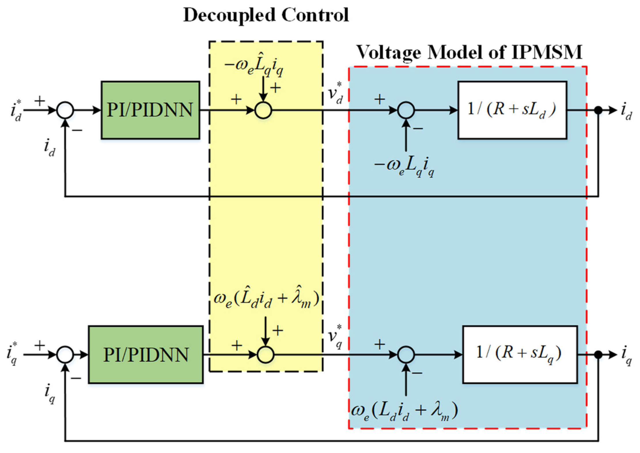
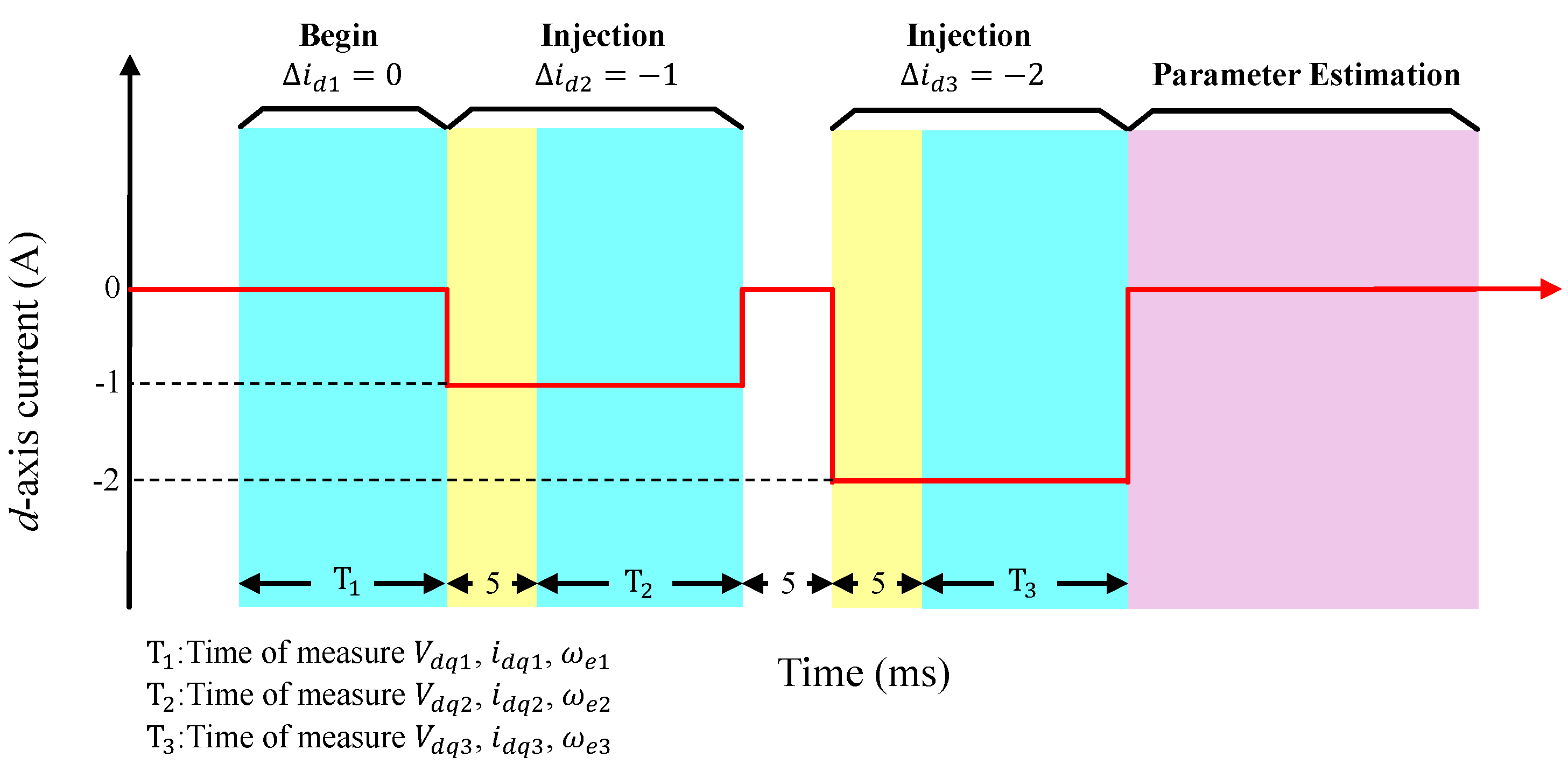
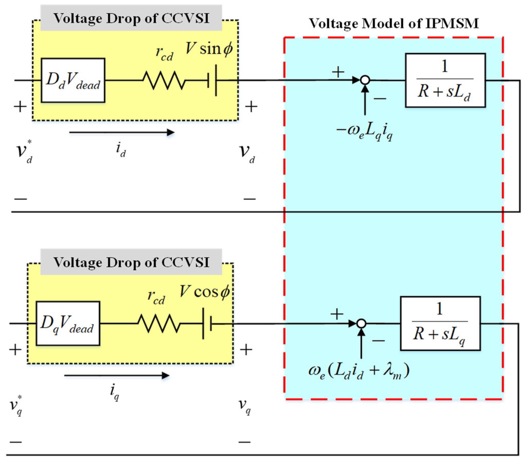
2.1. Voltage Model of IPMSM Based on d-Axis Current Injection
2.2. Estimation of Distorted Voltage Term
3. RLS Parameter Estimation Methodology
- (1).
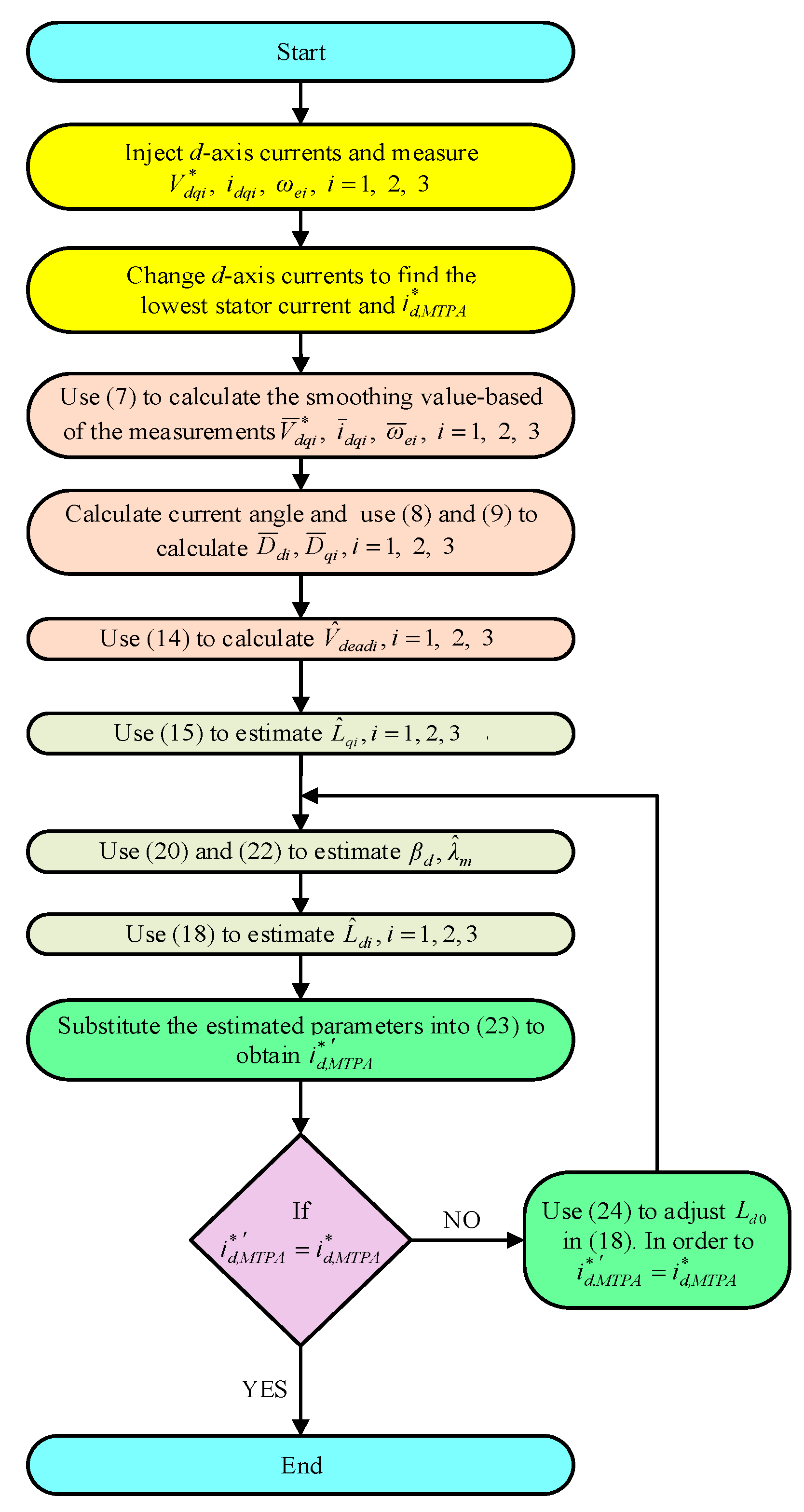
- Current injection: Inject d-axis currents and measure , i = 1, 2, 3.
- (2).
- Finding the lowest stator current: Change d-axis currents to find the lowest stator current and .
- (3).
- Smoothing: Use (7) to calculate the smoothing value-based of the measurements , i = 1, 2, 3.
- (4).
- Calculating distorted coefficients and voltage: Calculate current angle and use (8) and (9) to calculate , i = 1,2,3. Moreover, use (14) to calculate , i = 1, 2, 3.
- (5).
- q-axis inductance estimation: Use (15) to estimate , i = 1, 2, 3.
- (6).
- Parameters estimation: Use (20) and (22) to estimate , and use (18) to estimate , i = 1, 2, 3.
- (7).
- Verification: Substitute the estimated parameters into (23) to obtain to check if or not. If not, go to next step. If yes, then end the algorithm.
- (8).
- Adjusting: In order to achieve , use (24) to adjust in (18) and then go back to step 6.
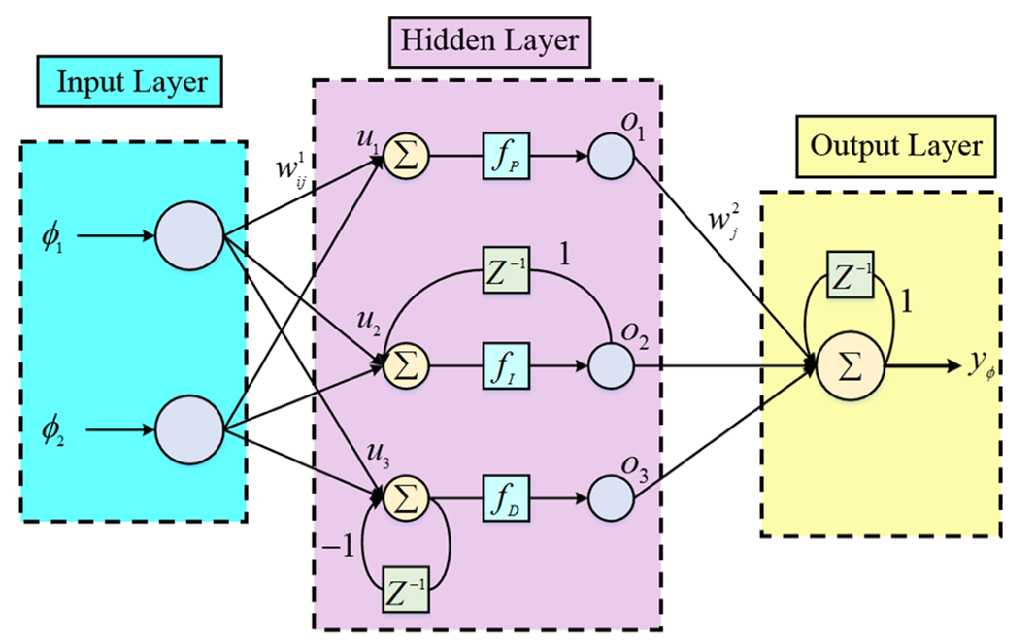
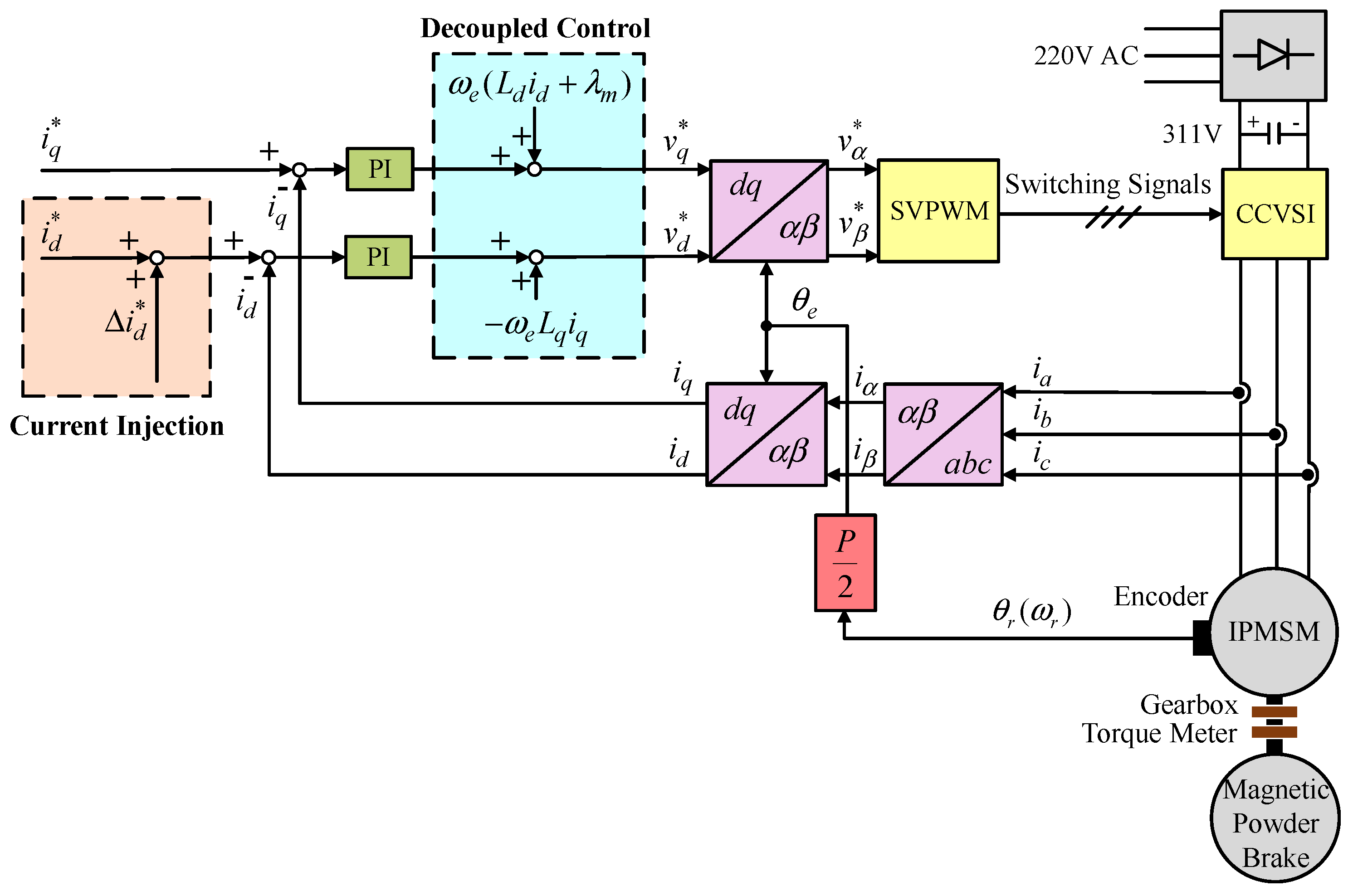
4. Current-Loop Control Using PID Neural Network Controller
- Layer 1 (input layer)
- Layer 2 (hidden layer)
- Layer 3 (output layer)
- Layer 3
- Layer 2
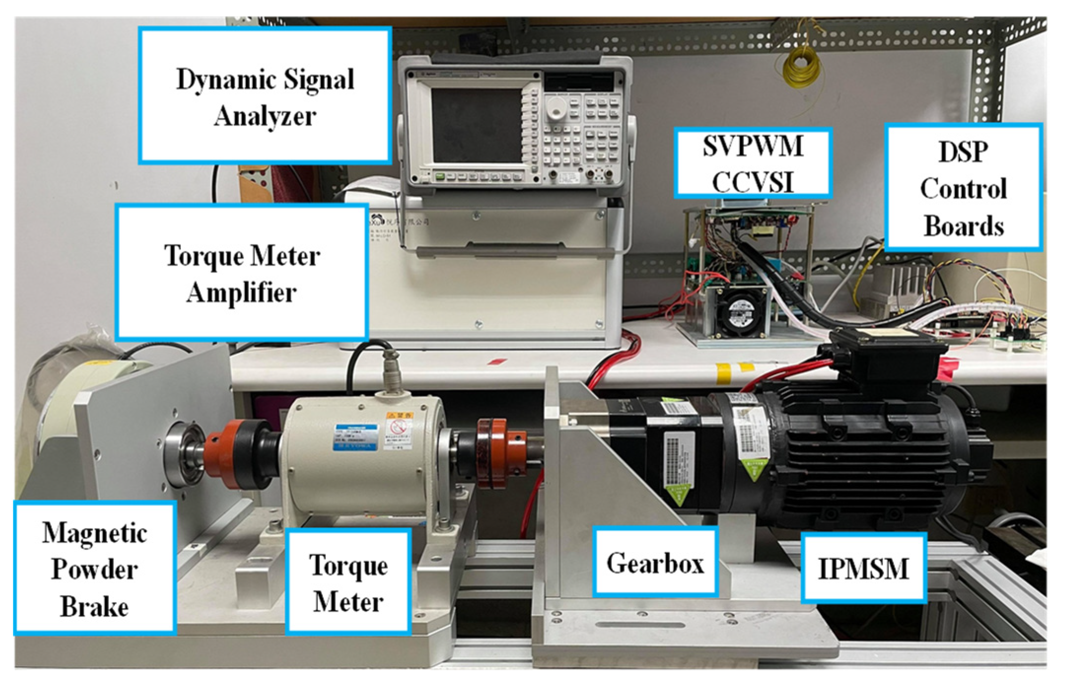
5. Experimentation
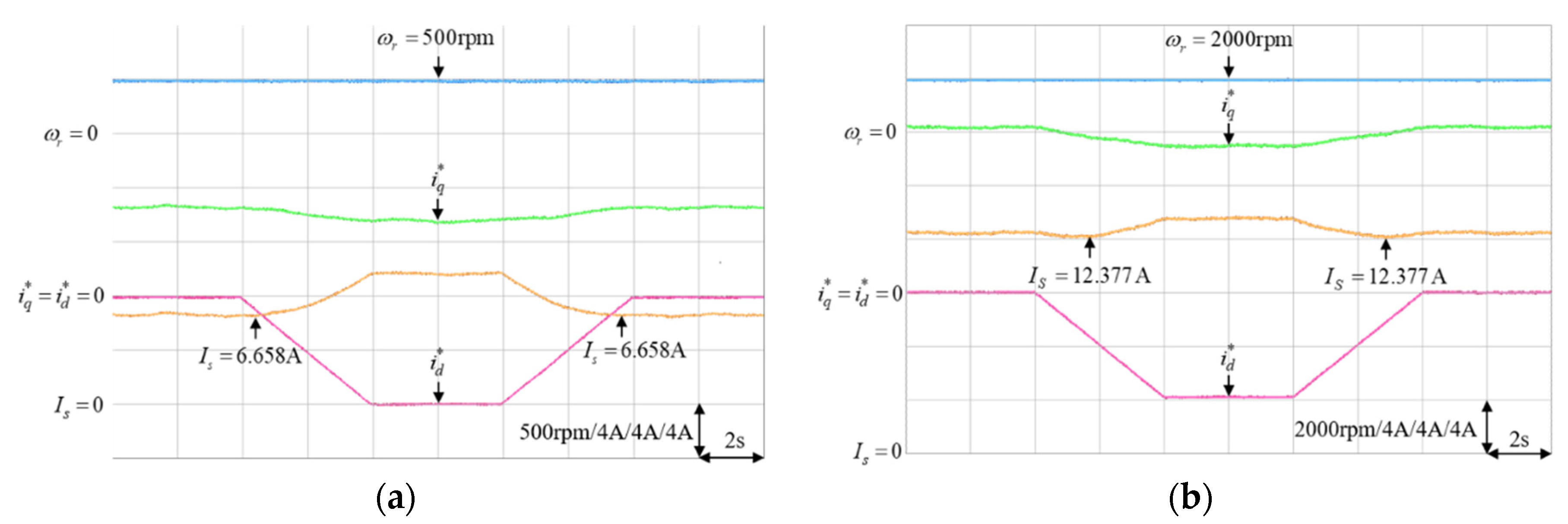
5.1. Online Parameter Estimation Using d-Axis Current Injection
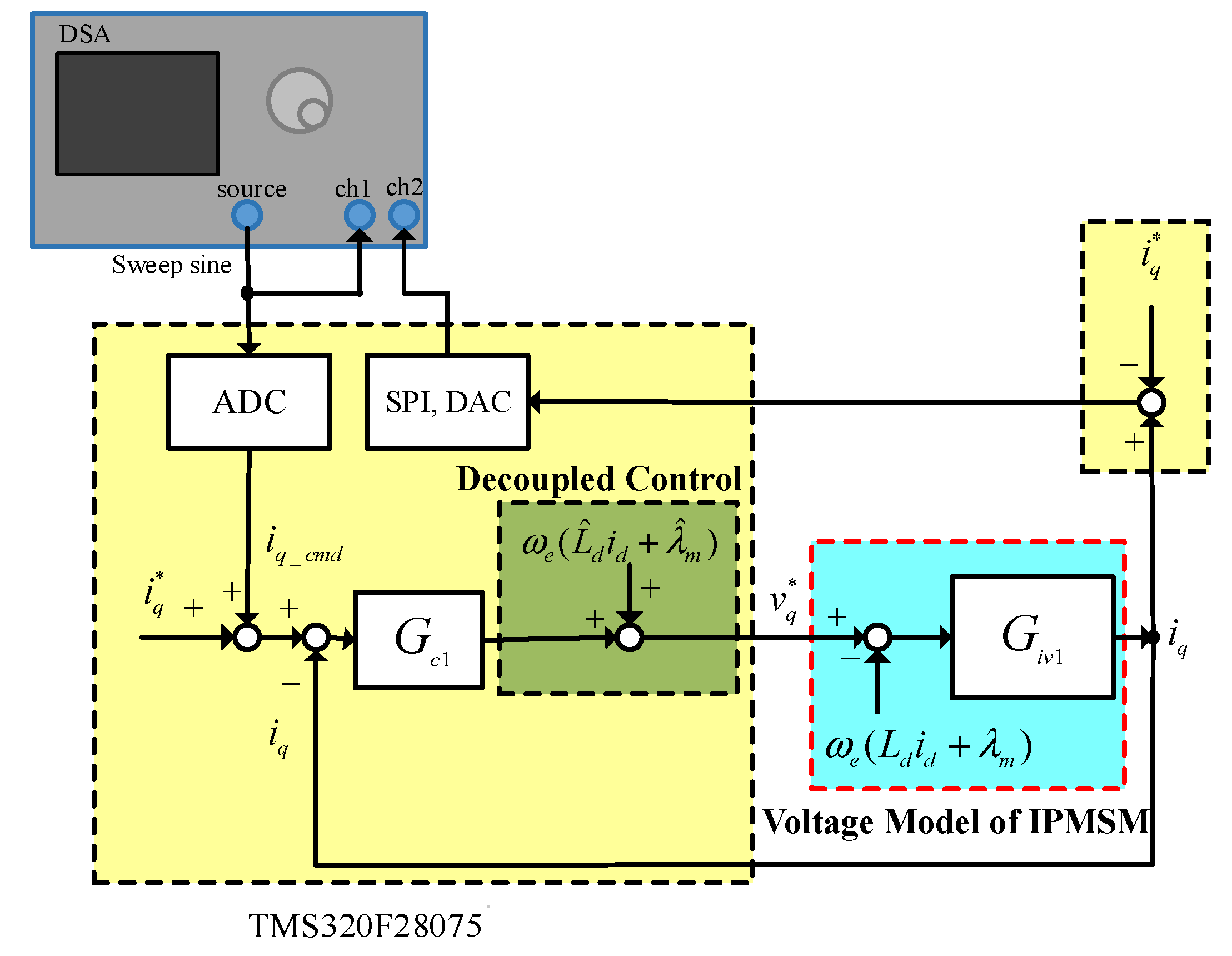
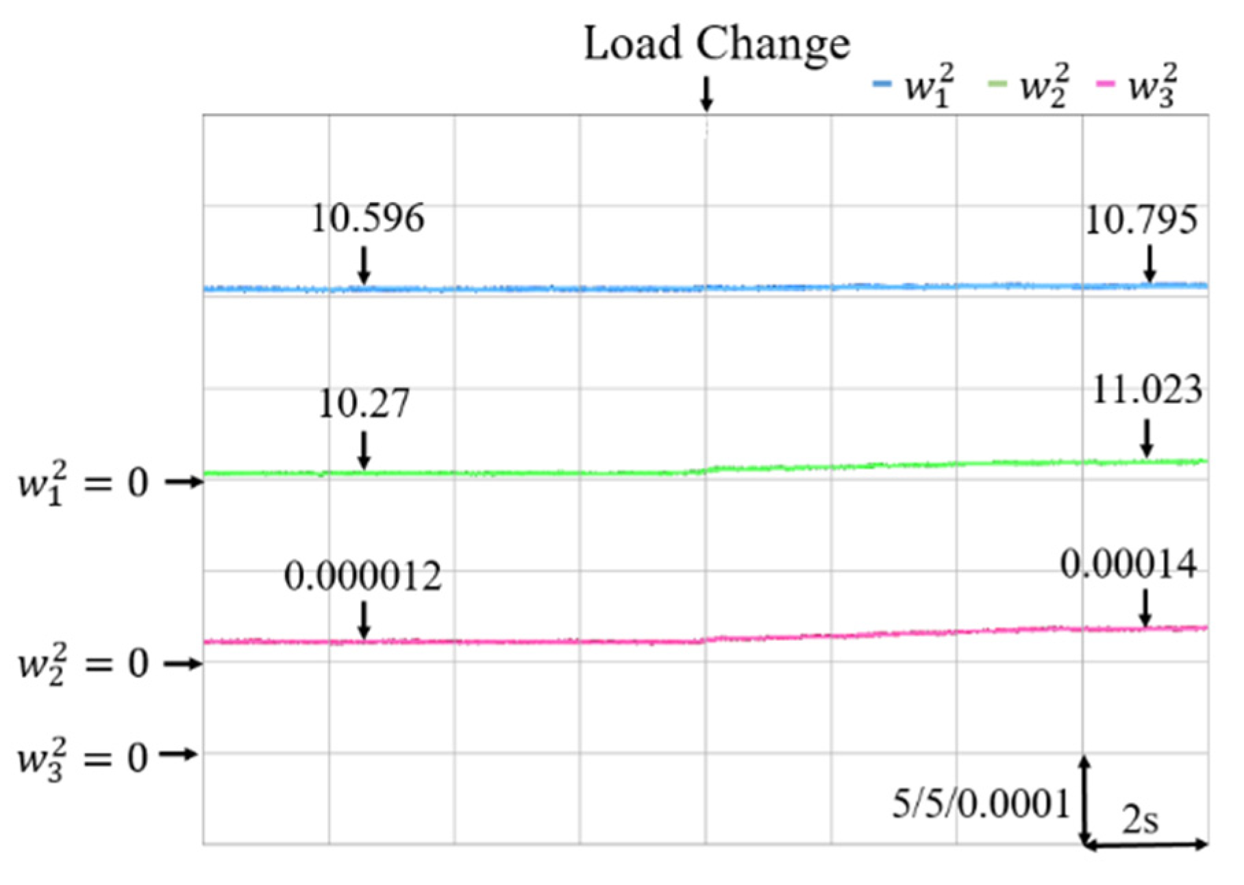
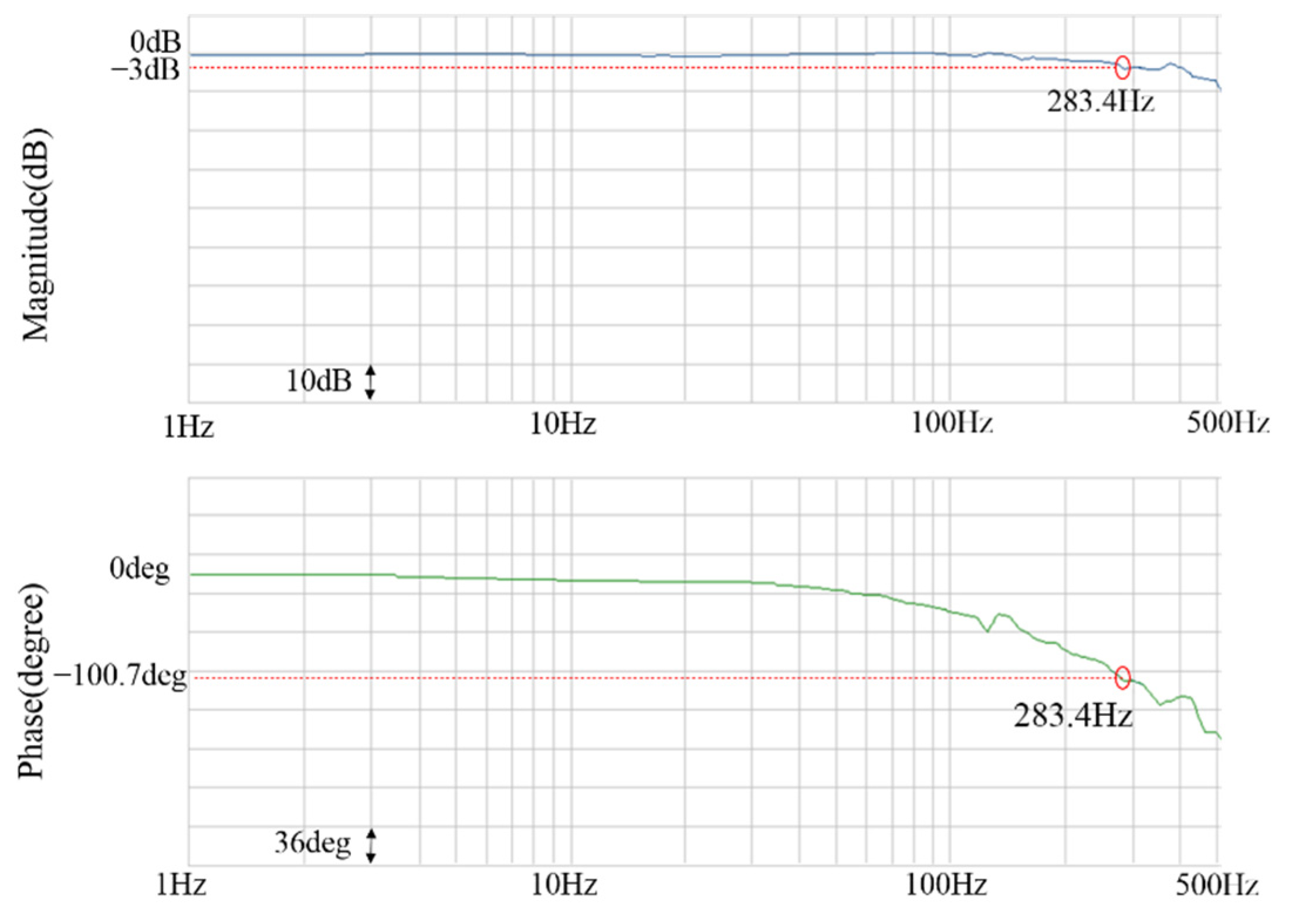
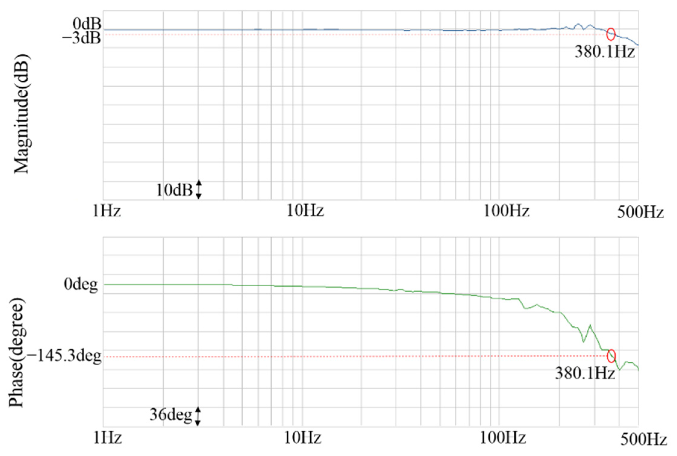
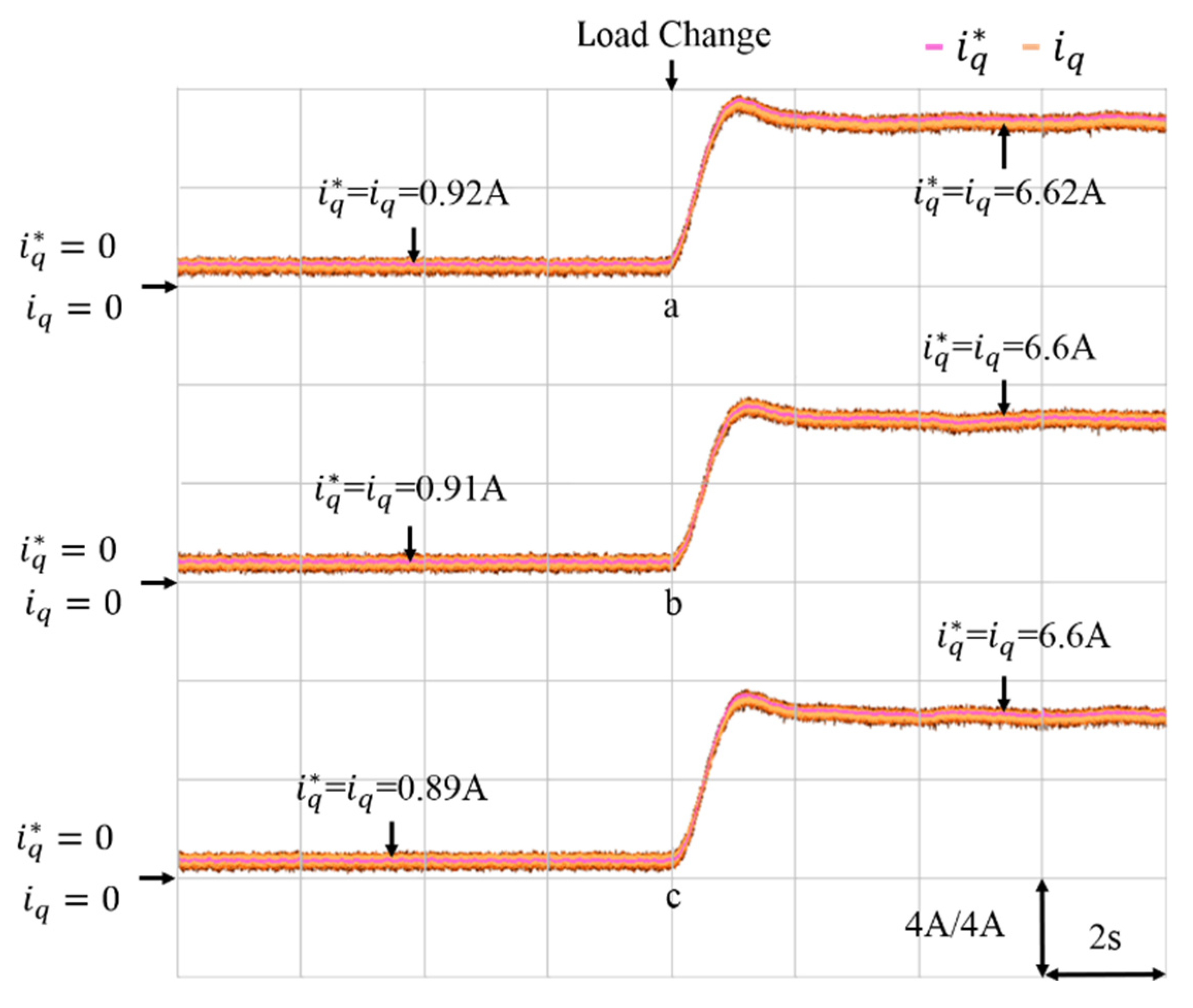
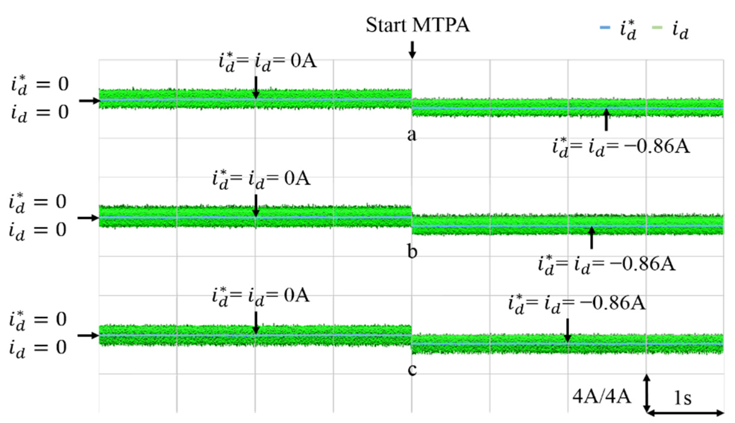
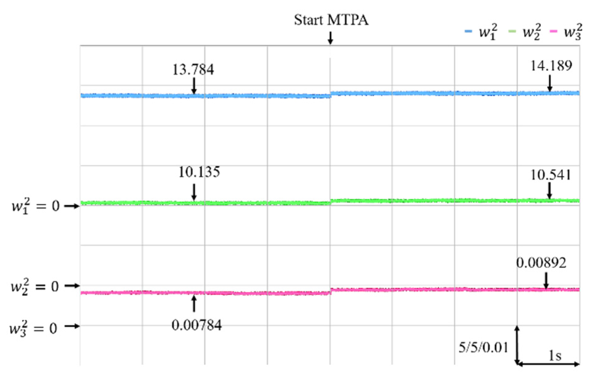
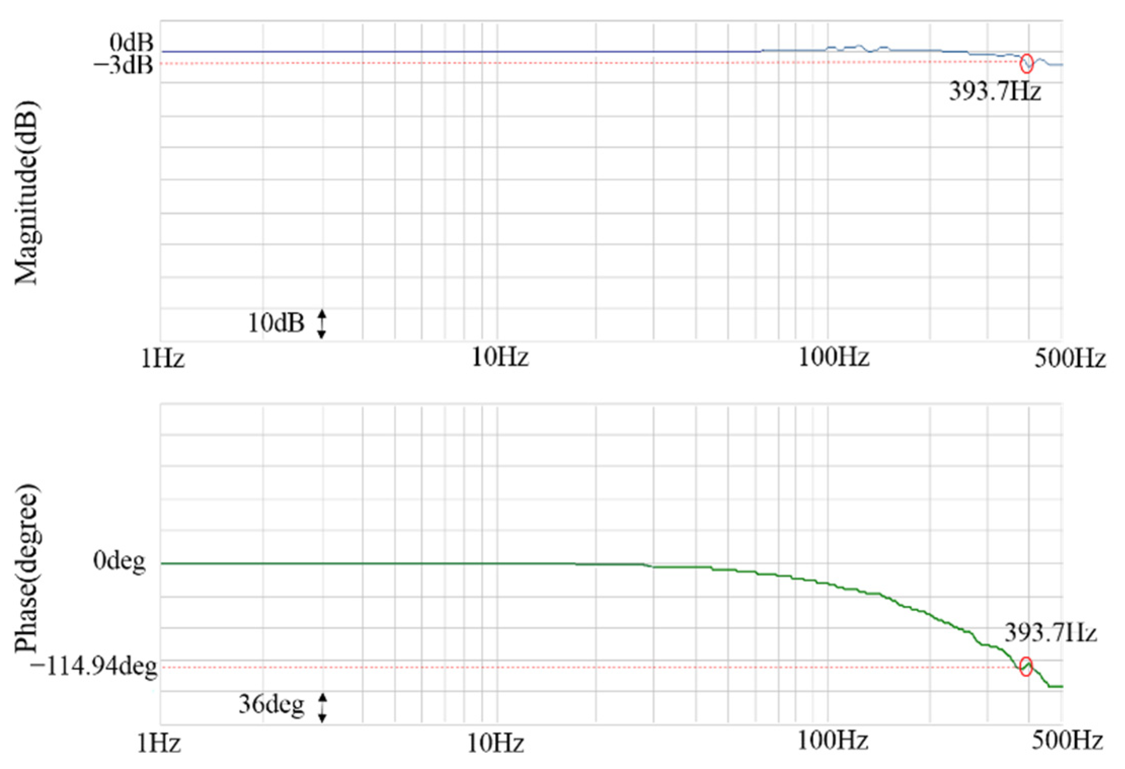
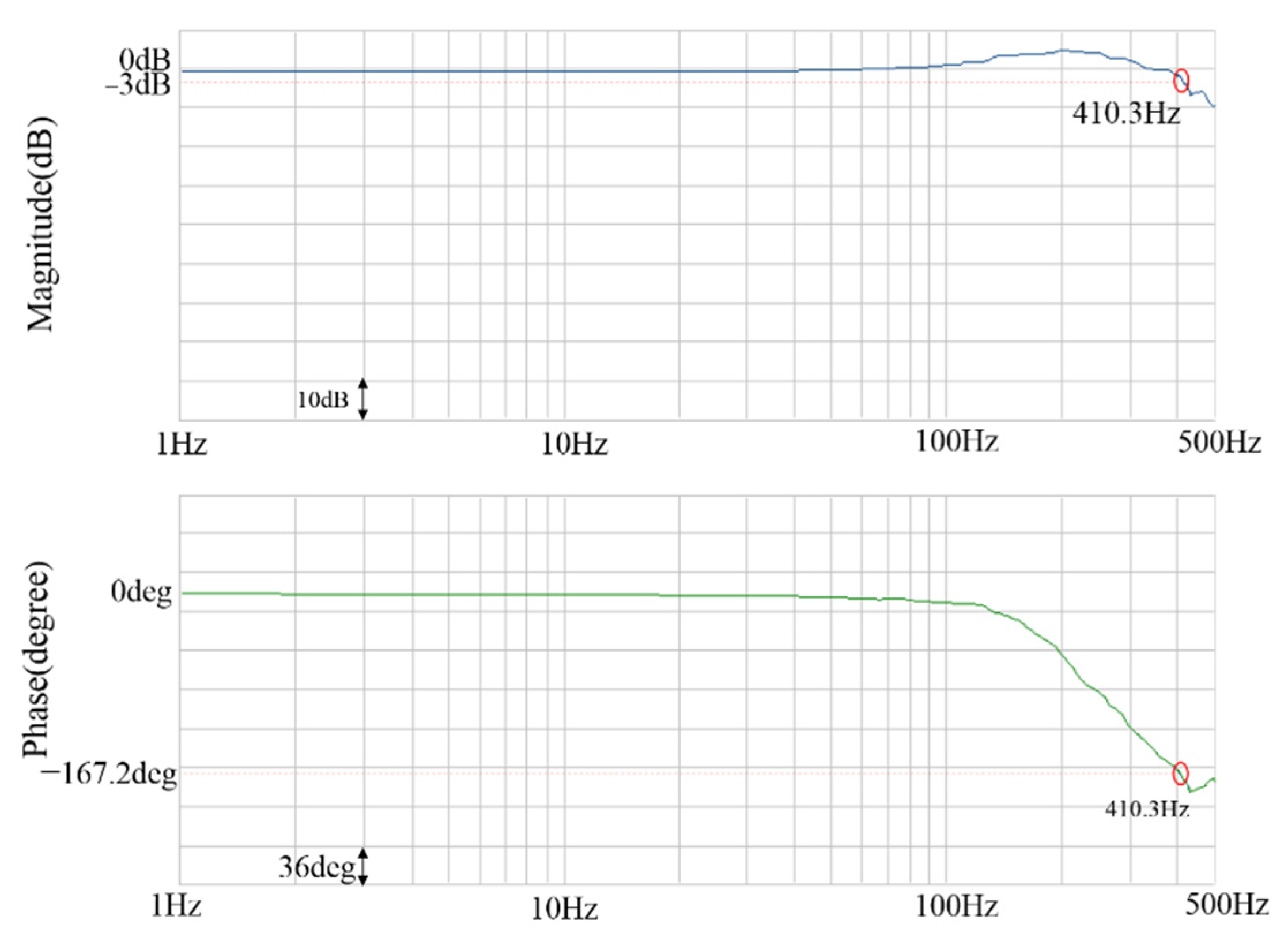
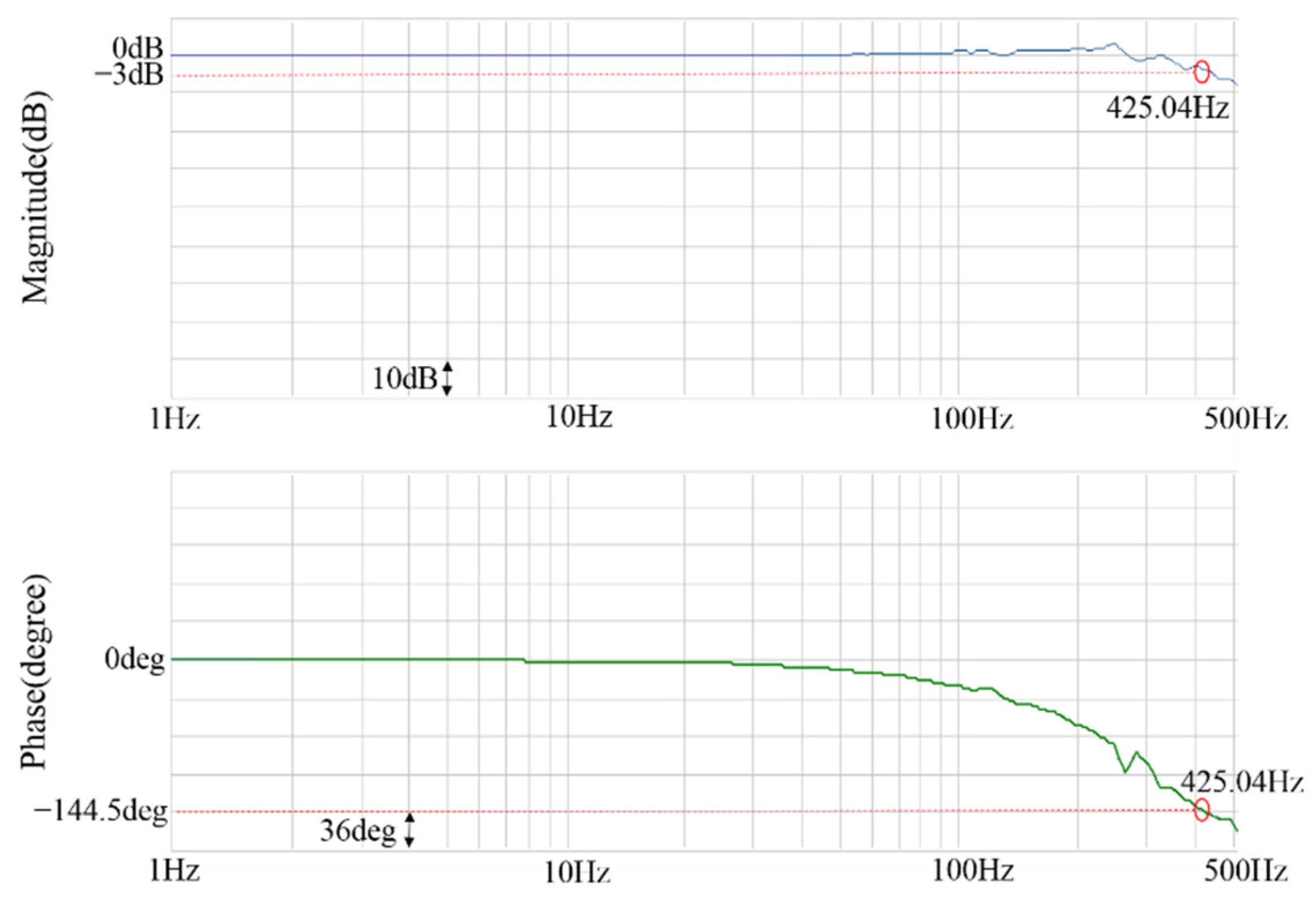
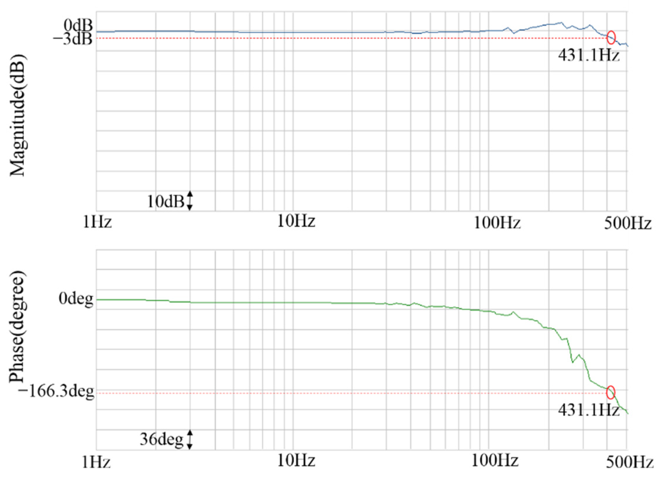
5.2. Enhanced Current-Loop Control Using PID Neural Network Controller
6. Conclusions
Author Contributions
Funding
Institutional Review Board Statement
Informed Consent Statement
Data Availability Statement
Conflicts of Interest
Appendix A
References
- Lin, F.J.; Hung, Y.C.; Chen, J.M.; Yeh, C.M. Sensorless IPMSM drive system using saliency back-EMF-based intelligent torque observer with MTPA control. IEEE Trans. Ind. Inform. 2014, 10, 1226–1241. [Google Scholar]
- Vandoorn, T.L.; Belie, F.M.D.; Vyncke, T.J.; Melkebeek, J.A.; Lataire, P. Generation of multisinusoidal test signals for the identification of synchronous-machine parameters by using a voltage-source inverter. IEEE Trans. Ind. Electron. 2010, 57, 430–439. [Google Scholar] [CrossRef]
- Rahman, K.M.; Hiti, S. Identification of machine parameters of a synchronous motor. IEEE Trans. Ind. Appl. 2005, 41, 557–565. [Google Scholar] [CrossRef]
- Dang, D.Q.; Rafaq, M.S.; Choi, H.H.; Jung, J.W. Online parameter estimation technique for adaptive control applications of interior PM synchronous motor drives. IEEE Trans. Ind. Electron. 2016, 63, 1438–1449. [Google Scholar] [CrossRef]
- Underwood, S.J.; Husain, I. Online parameter estimation and adaptive control of permanent-magnet synchronous machines. IEEE Trans. Ind. Electron. 2010, 57, 2435–2443. [Google Scholar] [CrossRef]
- Bui, M.X.; Rahman, M.F.; Guan, D.; Xiao, D. A new and fast method for on-line estimation of d and q axes inductances of interior permanent magnet synchronous machines using measurements of current derivatives and inverter DC-bus voltage. IEEE Trans. Ind. Electron. 2019, 66, 7488–7497. [Google Scholar] [CrossRef]
- Feng, G.D.; Lai, C.Y.; Mukherjee, K.; Kar, N.C. Current injection-based online parameter and VSI nonlinearity estimation for PMSM drives using current and voltage DC components. IEEE Trans. Transp. Electrif. 2016, 2, 119–128. [Google Scholar] [CrossRef]
- Wang, G.L.; Li, C.; Zhang, G.Q.; Xu, D.G. Self-adaptive stepsize affine projection based parameter estimation of IPMSM using square-wave current injection. CES Trans. Eng. Electr. Mach. Syst. 2017, 1, 48–57. [Google Scholar] [CrossRef]
- Zhu, Z.Q.; Liang, D.; Liu, K. Online parameter estimation for permanent magnet synchronous machines: An overview. IEEE Access 2021, 9, 59059–59084. [Google Scholar] [CrossRef]
- Liu, T.H.; Chen, Y.; Wu, M.J.; Dai, B.C. Adaptive controller for an MTPA IPMSM drive system without using a high-frequency sinusoidal generator. IET J. Eng. 2017, 2, 13–25. [Google Scholar] [CrossRef]
- Sun, T.; Wang, J.; Chen, X. Maximum torque per ampere (MTPA) control for interior permanent magnet synchronous machine drives based on virtual signal injection. IEEE Trans. Power Electron. 2015, 30, 5036–5045. [Google Scholar] [CrossRef]
- Dianov, A.; Anuchin, A.; Bodrov, A. Robust MTPA Control for Steady State Operation of Low-Cost IPMSM Drives. IEEE J. Emerg Sel. Top. Ind. Electron. 2021. early accessed. [Google Scholar] [CrossRef]
- Nadjai, Y.; Ahmed, H.; Takorabet, N.; Haghgooei, P. Maximum Torque per Ampere Control of Permanent Magnet Assisted Synchronous Reluctance Motor: An Experimental Study. Int. J. Robot. Control Syst. 2021, 1, 416–427. [Google Scholar]
- Lin, F.J.; Liao, Y.H.; Lin, J.R.; Lin, W.T. Interior permanent magnet synchronous motor drive system with machine learning-based maximum torque per ampere and flux-weakening control. Energies 2021, 14, 346. [Google Scholar] [CrossRef]
- Lin, F.J.; Chen, S.G.; Liu, Y.T.; Yu, W.A. Online autotuning of a servo drive using wavelet fuzzy neural network to search for the optimal bandwidth. IEEE SMC Mag. 2018, 4, 28–37. [Google Scholar] [CrossRef]
- Wang, H.J.; Yang, M.; Xu, D.G. Current-loop bandwidth expansion strategy for permanent magnet synchronous motor drives. In Proceedings of the 2010 5th IEEE Conference on Industrial Electronics and Applications, Taichung, Taiwan, 15–17 June 2010; pp. 1340–1345. [Google Scholar]
- Fuentes, E.J.; Rodriguez, J.; Silva, C.; Diaz, S.; Quevedo, D.E. Speed control of a permanent magnet synchronous motor using predictive current control. In Proceedings of the 2009 IEEE 6th International Power Electronics and Motion Control Conference, Wuhan, China, 17–20 May 2009; pp. 390–395. [Google Scholar]
- Ren, J.J.; Ye, Y.Q.; Xu, G.F.; Zhao, Q.S.; Zhu, M.Z. Uncertainty- and disturbance-estimator-based current control scheme for PMSM drives with a simple parameter tuning algorithm. IEEE Trans. Power Electron. 2017, 32, 5712–5722. [Google Scholar] [CrossRef]
- Chung, D.W.; Sul, S.K. Analysis and compensation of current measurement error in vector-controlled AC motor drives. IEEE Trans. IEEE Trans. Ind. Appl. 1998, 34, 340–345. [Google Scholar] [CrossRef]
- Lee, K.W.; Kim, S.I. Dynamic performance improvement of a current offset error compensator in current vector-controlled SPMSM drives. IEEE Trans. Ind. Electron. 2019, 66, 6727–6736. [Google Scholar] [CrossRef]
- Lin, F.J.; Liu, Y.T.; Yu, W.A. Power perturbation based MTPA with an online tuning speed controller for IPMSM drive system. IEEE Trans. Ind. Electron. 2018, 65, 3677–3687. [Google Scholar] [CrossRef]
- Chen, S.Y.; Li, T.H.; Chang, C.H. Intelligent fractional-order backstepping control for an ironless linear synchronous motor with uncertain nonlinear dynamics. ISA Trans. 2019, 89, 218–232. [Google Scholar] [CrossRef]
- Chen, S.Y.; Lin, F.J. Decentralized PID neural network control for five degree-of-freedom active magnetic bearing. Eng. Appl. Artif. Intell. 2013, 26, 962–973. [Google Scholar] [CrossRef]
- Kim, H.W.; Youn, M.J.; Cho, K.Y.; Kim, H.S. Nonlinearity estimation and compensation of PWM VSI for PMSM under resistance and flux linkage uncertainty. IEEE Trans. Control Syst. Technol. 2006, 14, 589–601. [Google Scholar]
- Lee, K.D.; Lee, H.W.; Lee, J.; Kim, W.H. Analysis of motor performance according to the inductance design of IPMSM. IEEE Trans. Magn. 2015, 51, 1–4. [Google Scholar]
- Lin, F.J.; Hung, Y.C.; Tsai, M.T. Fault-Tolerant Control for Six-Phase PMSM Drive System via Intelligent Complementary Sliding-Mode Control Using TSKFNN-AMF. IEEE Trans. Ind. Electron. 2013, 60, 5747–5762. [Google Scholar] [CrossRef]


| Items | Units | Quantities |
|---|---|---|
| Torque | Nm | 50 |
| Rated current | A | 2.15 |
| Coil resistance | Ohm | 11.14 |
| Mass of powder | g | 60 |
| Maximum rotating speed | rpm | 1800 |
| Items | Units | Quantities |
|---|---|---|
| Pole number | 8 | |
| Rated power | W | 2000 |
| Rated line voltage | V | 220 |
| Rated current | A | 10.6 |
| Rated torque | Nm | 9.5 |
| Rated speed | rpm | 2000 |
| d-axis inductance | mH | 3.48 |
| q-axis inductance | mH | 6.16 |
| Magnetic flux | Wb | 0.143 |
| Resistance | ohm | 0.57 |
| Viscous damping | Nm/(rad/sec) | |
| Inertia | Nm/(rad/sec2) |
| 500 rpm 4.75 Nm | 500 rpm 9.5 Nm | 1000 rpm 4.75 Nm | 1000 rpm 9.5 Nm | 1500 rpm 4.75 Nm | 1500 rpm 9.5 Nm | 2000 rpm 4.75 Nm | 2000 rpm 9.5 Nm | |
|---|---|---|---|---|---|---|---|---|
| 0.006065 | 0.005272 | 0.006593 | 0.005528 | 0.007246 | 0.005853 | 0.007618 | 0.006175 | |
| 0.003484 | 0.003486 | 0.003479 | 0.003481 | 0.003479 | 0.003478 | 0.003473 | 0.003483 | |
| 0.11625 | 0.12135 | 0.11367 | 0.11507 | 0.11766 | 0.11081 | 0.10969 | 0.10768 | |
| −0.9654 | −2.3322 | −1.2915 | −2.8142 | −1.4951 | −3.2417 | −1.6706 | −3.5572 | |
| −0.86 | −2.6893 | −0.86 | −2.6893 | −0.86 | −2.6893 | −0.86 | −2.6893 |
| 500 rpm 4.75 Nm | 500 rpm 9.5 Nm | 1000 rpm 4.75 Nm | 1000 rpm 9.5 Nm | 1500 rpm 4.75 Nm | 1500 rpm 9.5 Nm | 2000 rpm 4.75 Nm | 2000 rpm 9.5 Nm | |
|---|---|---|---|---|---|---|---|---|
| Times of 2nd order RLS | 1414 | 1428 | 438 | 434 | 1549 | 1546 | 949 | 948 |
| 500 rpm 4.75 Nm | 500 rpm 9.5 Nm | 1000 rpm 4.75 Nm | 1000 rpm 9.5 Nm | 1500 rpm 4.75 Nm | 1500 rpm 9.5 Nm | 2000 rpm 4.75 Nm | 2000 rpm 9.5 Nm | |
|---|---|---|---|---|---|---|---|---|
| 0.006065 | 0.005272 | 0.006593 | 0.005528 | 0.007246 | 0.005853 | 0.007618 | 0.006175 | |
| 0.003776 | 0.003191 | 0.004539 | 0.003578 | 0.005134 | 0.003924 | 0.005557 | 0.004207 | |
| 0.11636 | 0.12122 | 0.11482 | 0.11518 | 0.11263 | 0.11088 | 0.11091 | 0.10805 | |
| −0.8591 | −2.6890 | −0.8600 | −2.6899 | −0.8599 | −2.6884 | −0.8596 | −2.6895 | |
| −0.86 | −2.6893 | −0.86 | −2.6893 | −0.86 | −2.6893 | −0.86 | −2.6893 |
| 500 rpm 4.75 Nm | 500 rpm 9.5 Nm | 1000 rpm 4.75 Nm | 1000 rpm 9.5 Nm | 1500 rpm 4.75 Nm | 1500 rpm 9.5 Nm | 2000 rpm 4.75 Nm | 2000 rpm 9.5 Nm | |
|---|---|---|---|---|---|---|---|---|
| Times of 2nd order RLS | 1549 | 1431 | 581 | 476 | 1964 | 1733 | 1280 | 1158 |
Publisher’s Note: MDPI stays neutral with regard to jurisdictional claims in published maps and institutional affiliations. |
© 2021 by the authors. Licensee MDPI, Basel, Switzerland. This article is an open access article distributed under the terms and conditions of the Creative Commons Attribution (CC BY) license (https://creativecommons.org/licenses/by/4.0/).
Share and Cite
Lin, F.-J.; Chen, S.-Y.; Lin, W.-T.; Liu, C.-W. An Online Parameter Estimation Using Current Injection with Intelligent Current-Loop Control for IPMSM Drives. Energies 2021, 14, 8138. https://doi.org/10.3390/en14238138
Lin F-J, Chen S-Y, Lin W-T, Liu C-W. An Online Parameter Estimation Using Current Injection with Intelligent Current-Loop Control for IPMSM Drives. Energies. 2021; 14(23):8138. https://doi.org/10.3390/en14238138
Chicago/Turabian StyleLin, Faa-Jeng, Syuan-Yi Chen, Wei-Ting Lin, and Chih-Wei Liu. 2021. "An Online Parameter Estimation Using Current Injection with Intelligent Current-Loop Control for IPMSM Drives" Energies 14, no. 23: 8138. https://doi.org/10.3390/en14238138
APA StyleLin, F.-J., Chen, S.-Y., Lin, W.-T., & Liu, C.-W. (2021). An Online Parameter Estimation Using Current Injection with Intelligent Current-Loop Control for IPMSM Drives. Energies, 14(23), 8138. https://doi.org/10.3390/en14238138