
Empirical Estimation of the Energy Impacts of Projects Installed through Residential Property Assessed Clean Energy Financing Programs in California

Abstract
:1. Introduction
2. Materials and Methods
2.1. R-PACE Projects and Measures
2.2. Utility Electricity and Gas Usage Data for R-PACE Households
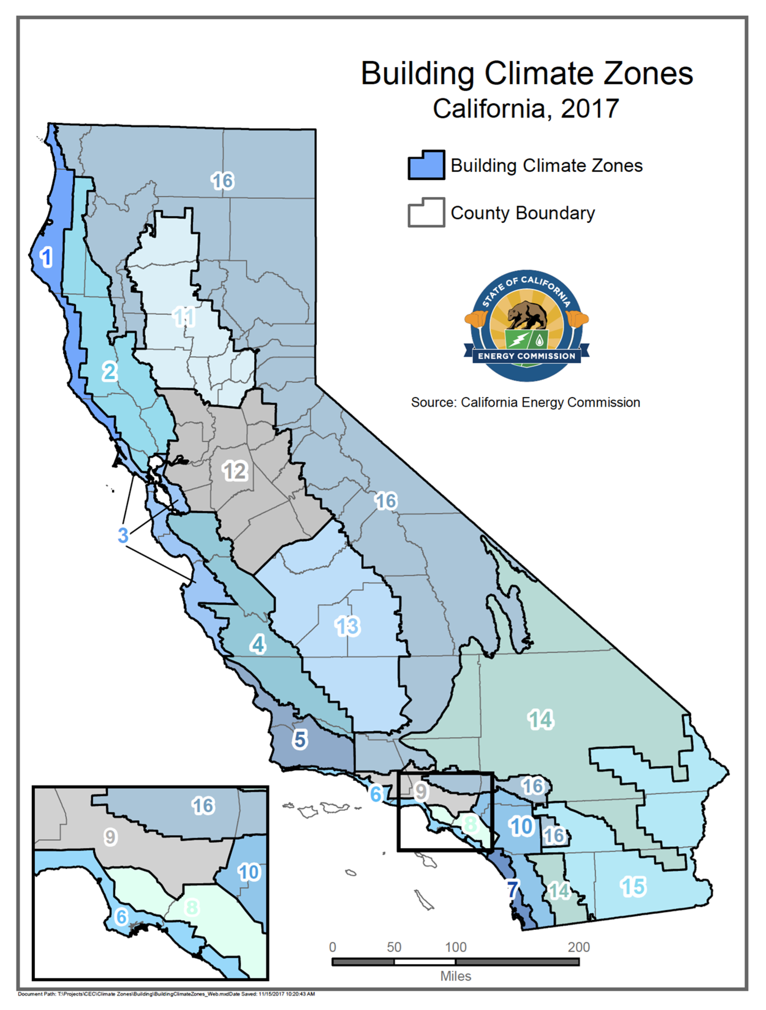
2.3. Temperature Data
2.4. Modeling of Energy Usage Impacts
- First, we fit a regression of gas usage on historical heating degree days in the baseline period to estimate the pre-project temperature dependency of the household’s gas usage.
- Second, we fit a regression of observed gas usage on historical heating degree days in the reporting period to estimate the post-project temperature dependency of the household’s gas usage.
- Third, we use the reporting period normal-year heating degree days as inputs into the models produced in the first two steps. The model then estimates post-project usage in a normal weather year and estimates what usage would have been had the project not occurred, using heating degree days in a normal year.
- Fourth, we subtract weather-normalized gas usage during the reporting period from the baseline period to estimate changes in gas usage because of the R-PACE project.
2.5. Defining Project Installation Dates
2.6. Selection of Comparison Households
- For each R-PACE household, we identify other R-PACE households that meet all of the following criteria:
- Their project start and end dates are outside the baseline and reporting periods of the household being matched (such that their usage was not affected by projects installed during the time period of comparison);
- They are in the same zip code and utility jurisdiction at the household being matched (and therefore may be subject to similar factors affecting energy usage, including prices and economic factors);
- Their usage (for the fuel in question) and weather data pass our data quality and sufficiency checks (see Appendix A for details); and
- They did not have solar PV installed before or during the baseline and reporting periods of the household being matched (because the presence of PV significantly alters the level and pattern of electricity usage in households).
- Of these potential candidates, we selected the household that had the most similar usage (electricity or gas, as appropriate) during the matched project’s baseline period as measured by the minimum sum of absolute differences in monthly consumption of that fuel over the R-PACE household’s baseline period. This prioritizes comparison households with similar monthly consumption to the matched household.
3. Results
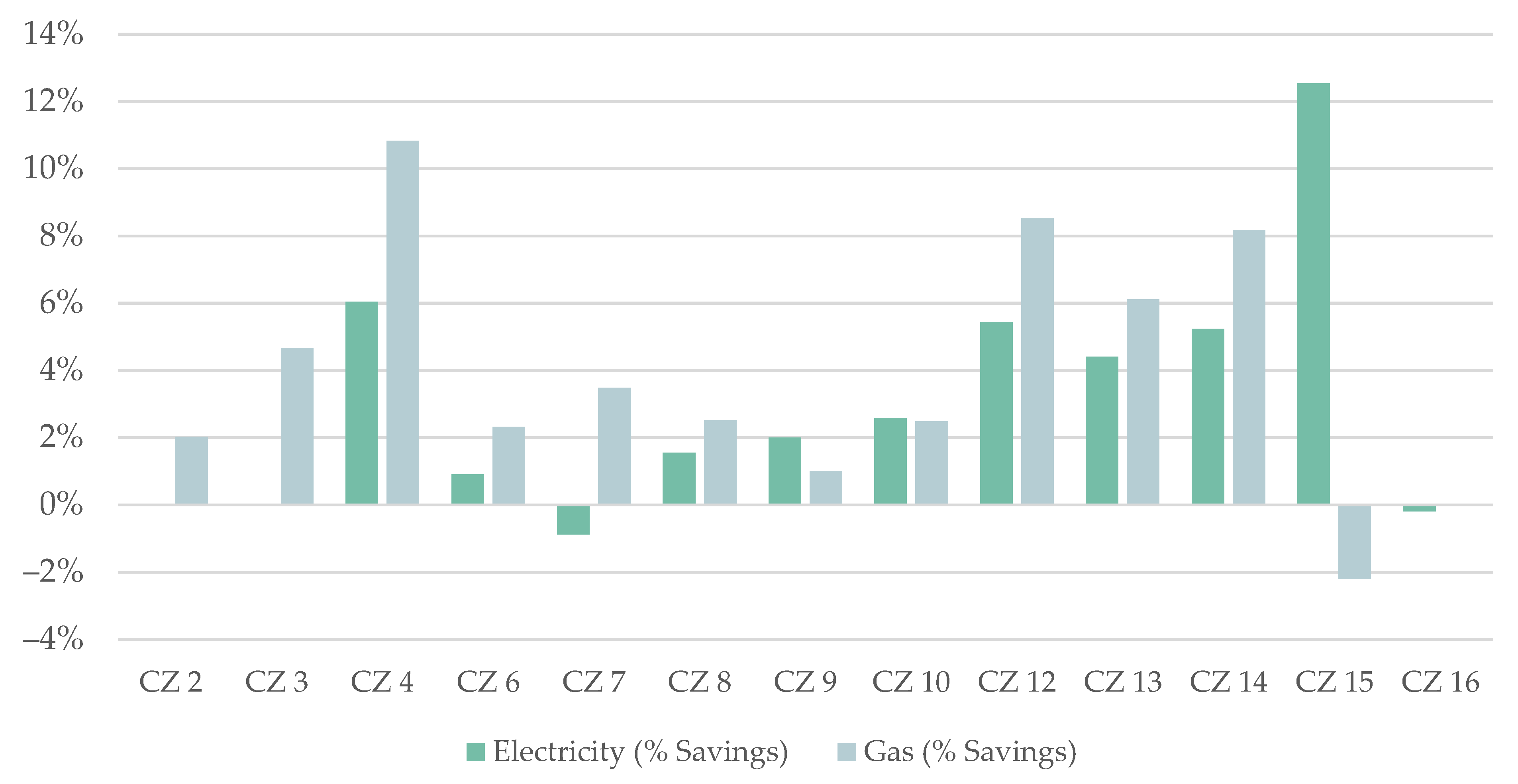
3.1. Usage Impacts by Utility
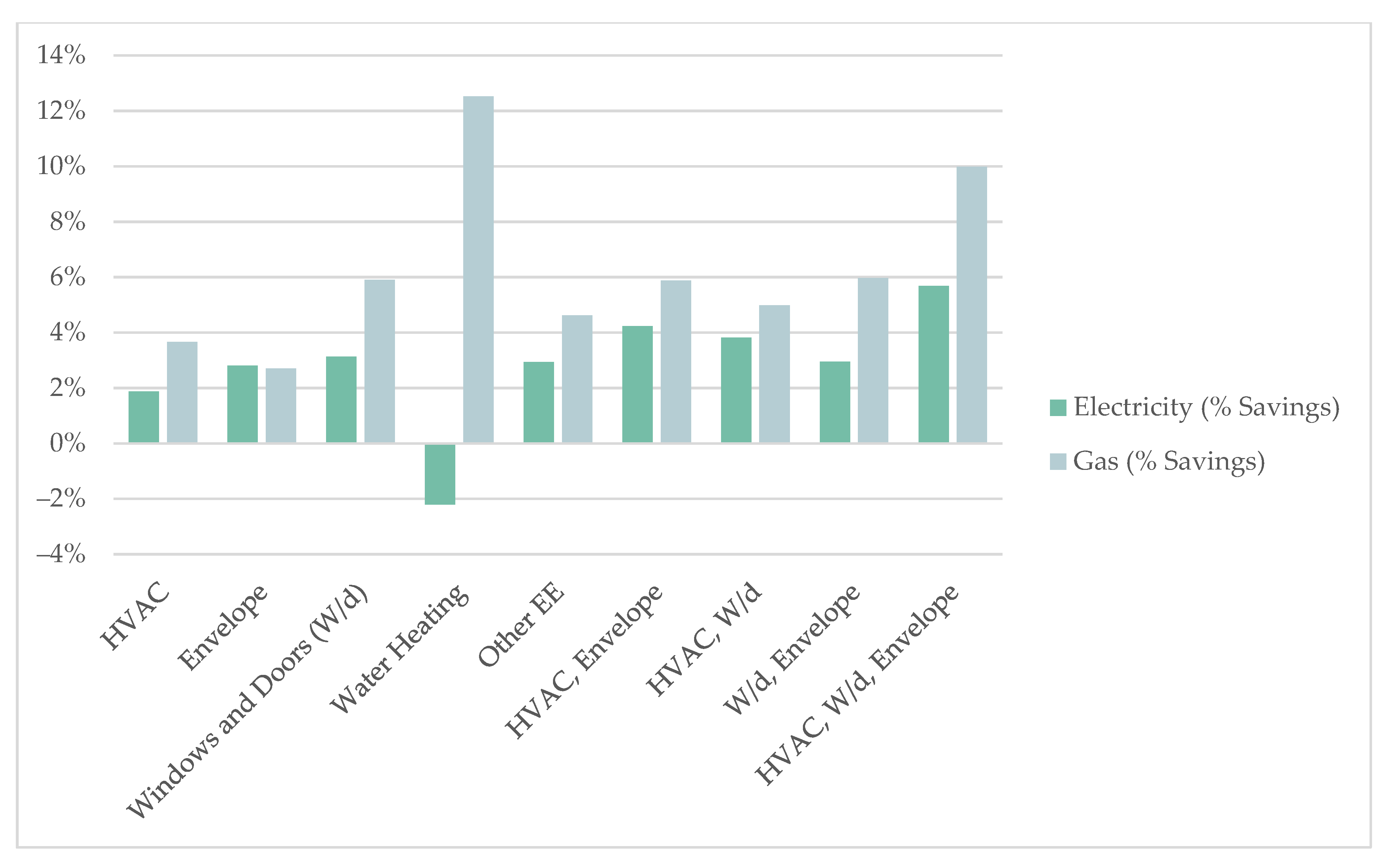
3.2. Usage Impacts by Energy Efficiency Measure Category
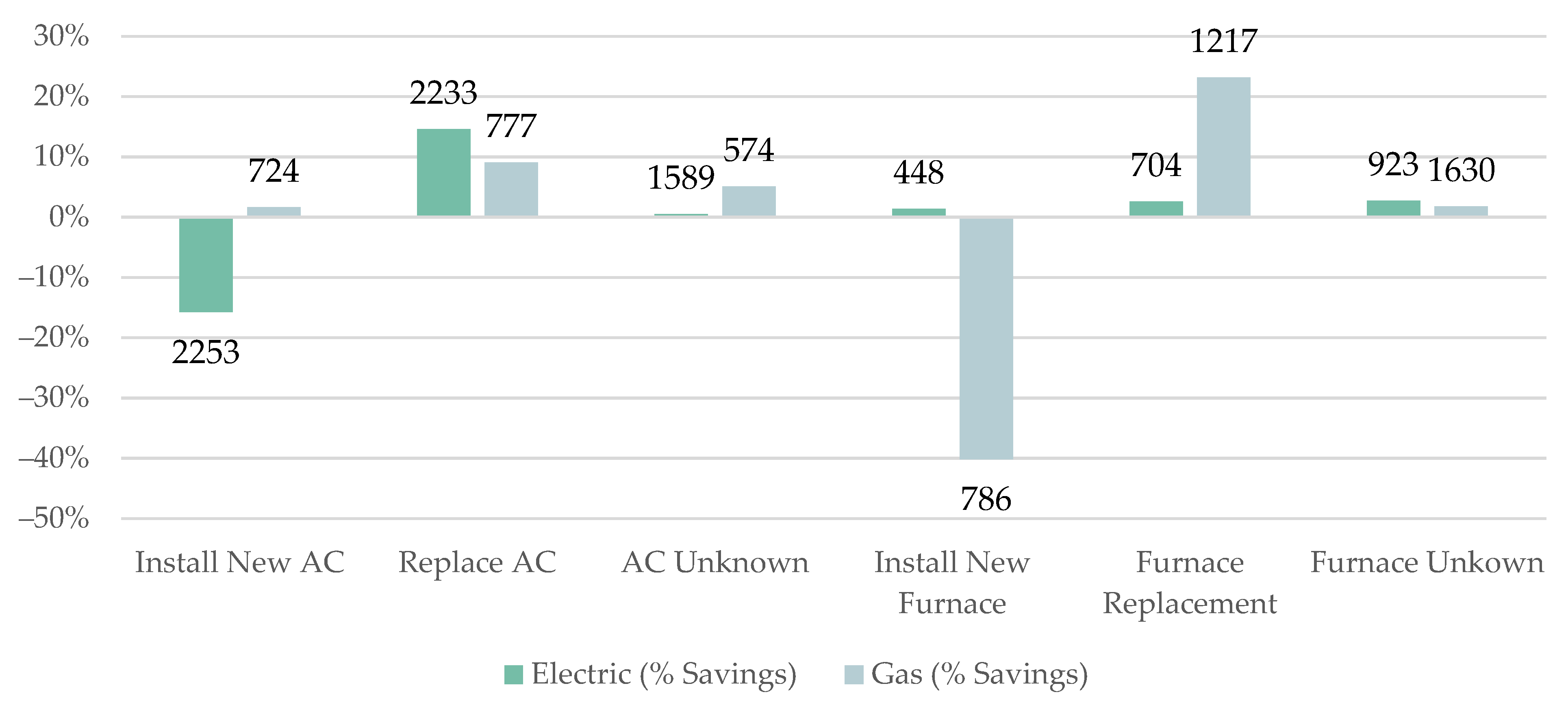
3.3. HVAC Project Savings
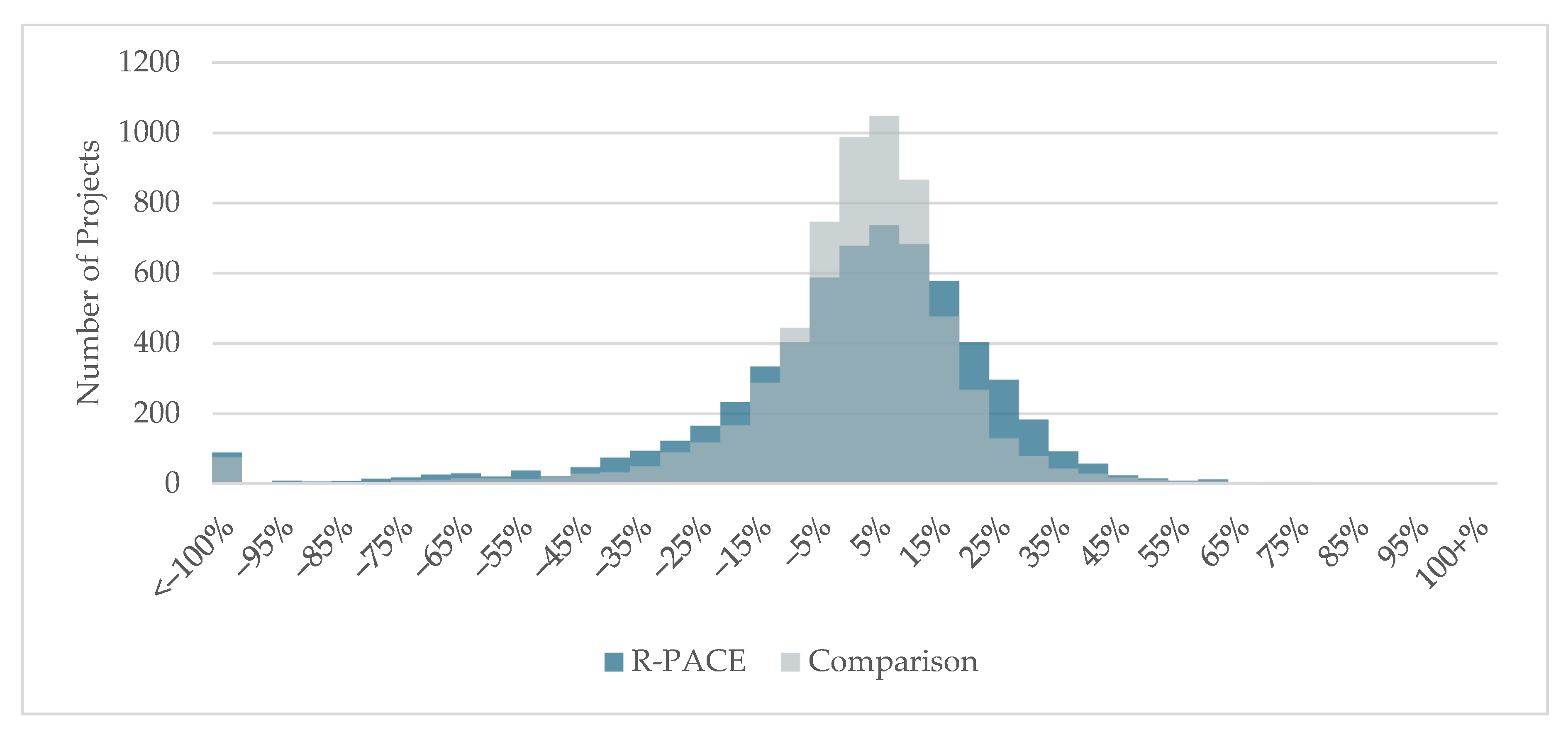
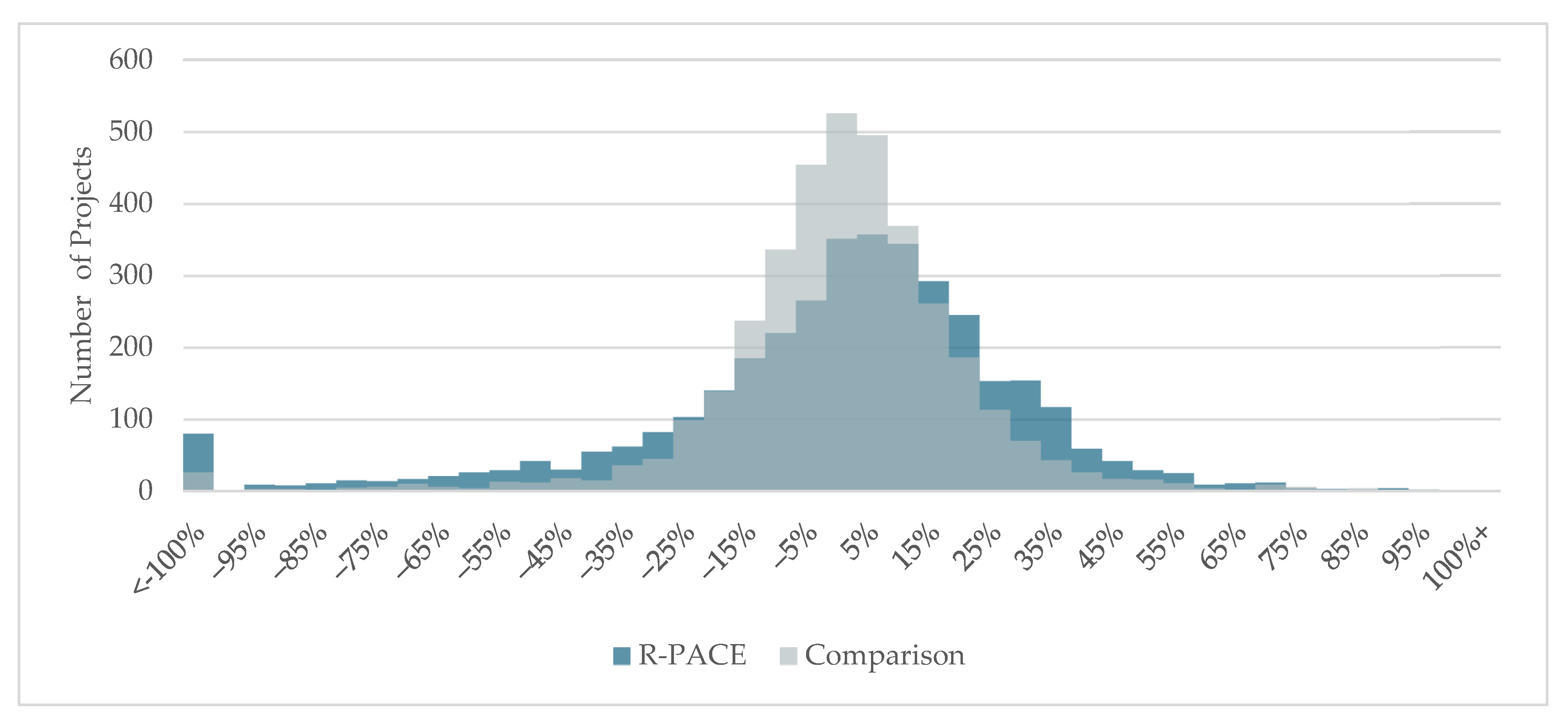
3.4. Usage Impacts across the R-PACE Portfolio
4. Discussion
4.1. The California Context
4.2. Comparison to Home Upgrade Program and Advanced Home Upgrade Program Impacts
4.3. Program-Level Impacts
4.4. Adoption of Energy Efficiency Equipment and Solar PV in Financing Programs
4.5. NMEC at Scale
5. Conclusions
Author Contributions
Funding
Institutional Review Board Statement
Informed Consent Statement
Data Availability Statement
Acknowledgments
Conflicts of Interest
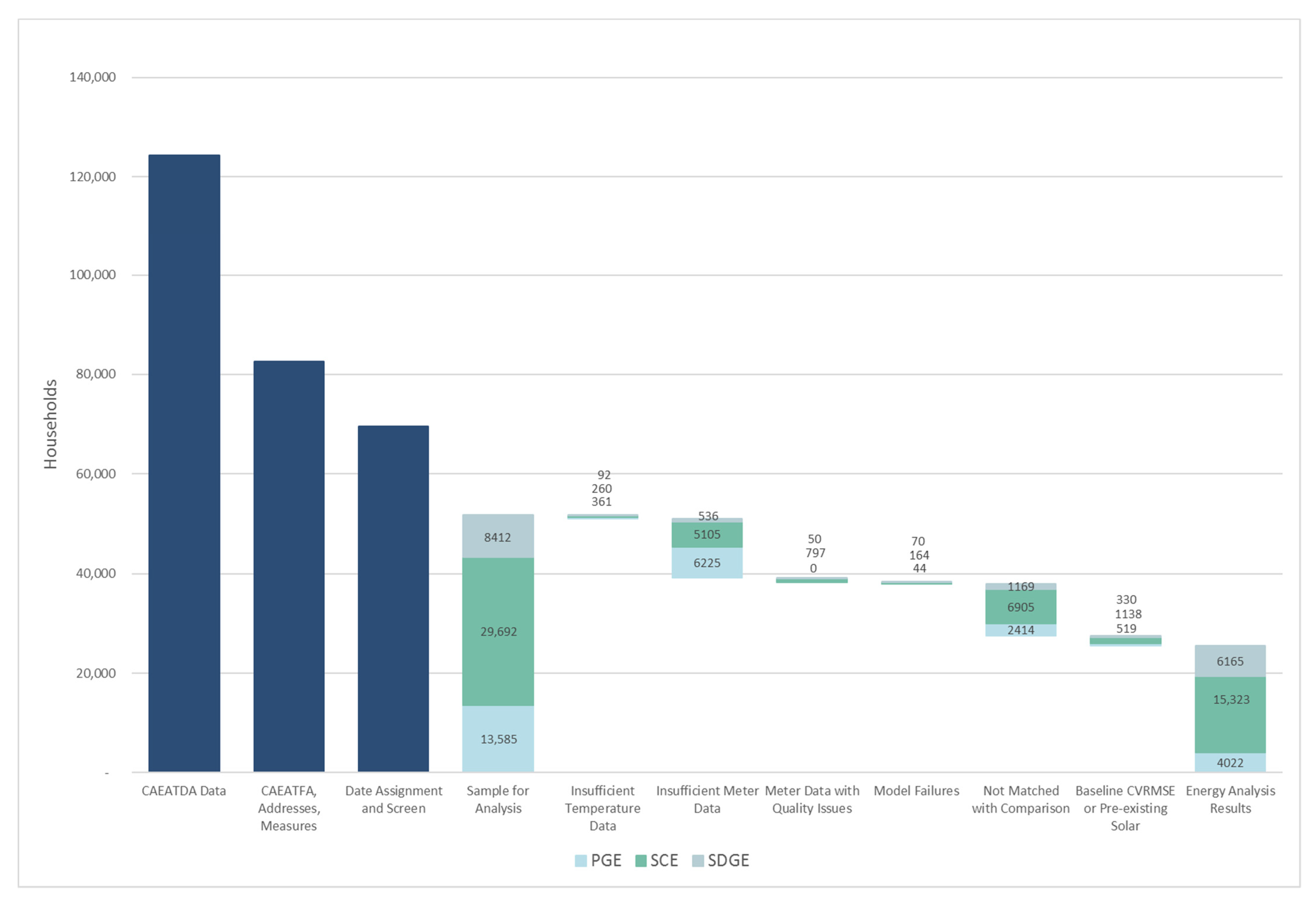
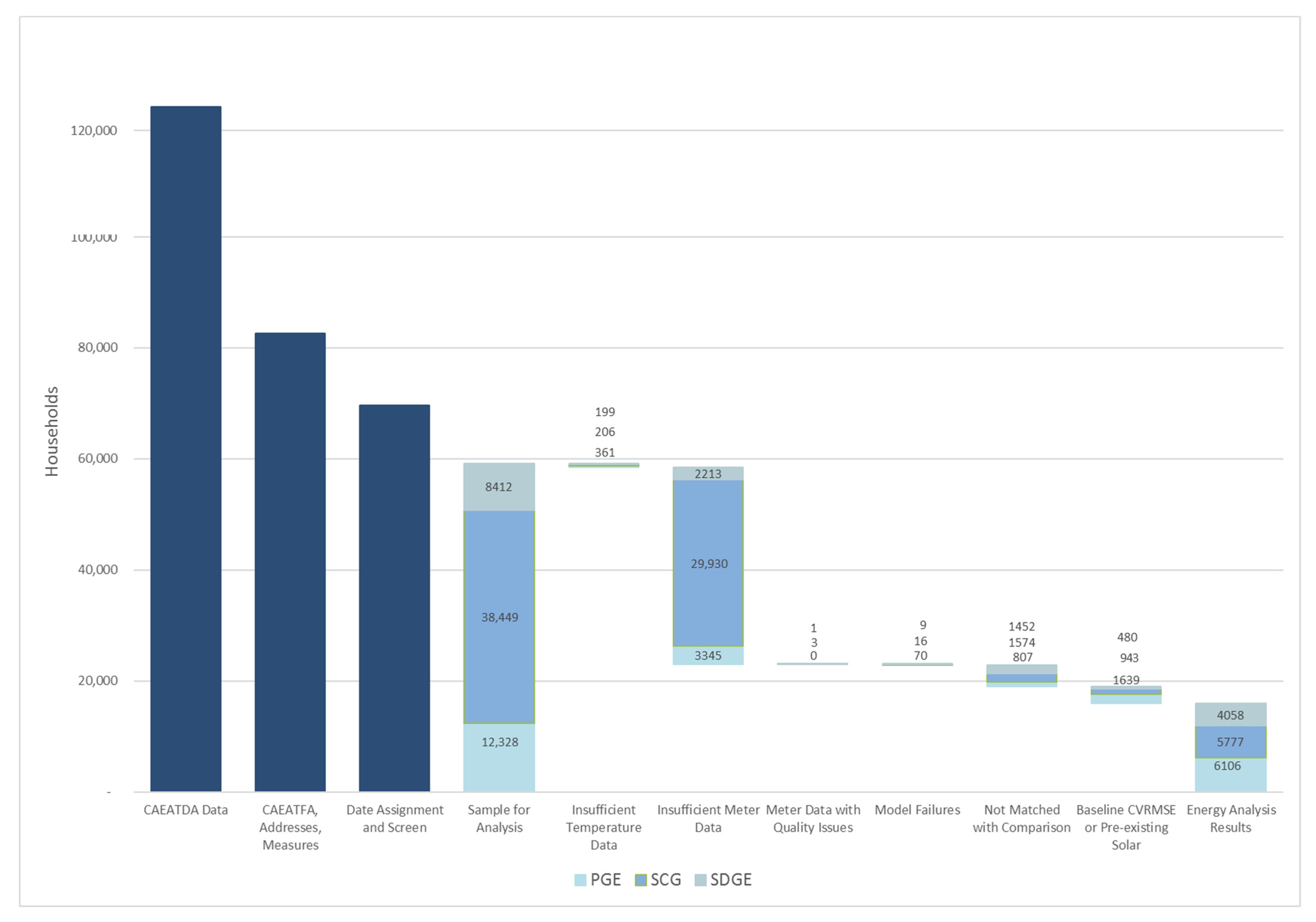
Appendix A. Data Quality Screening and Sample Size Attrition
- The temporal resolution of the data ranged from every 15 min (SCE) to hourly (PG&E electric, SDG&E electric, SCG) to daily (PG&E gas) to monthly (SDG&E gas).
- We received account-level data from some utilities and premise-level data from others. Whereas accounts identify the customer paying for a given fuel at a given premise, the premise identifies the location where accounts exist. We chose to conduct a premise-level analysis. As houses change occupancy, so do utility accounts, so an account-level analysis would have introduced breaks in metering time series and further restricted the number of households in our analysis. Moreover, the installed measures may influence energy usage even after a change in occupancy. Our use of a comparison group also helps guard against misinterpreting occupancy effects as project effects: comparison households may also have experienced occupancy-related impacts, and we would expect such occupancy-related impacts in the R-PACE group to be offset by similar impacts in the comparison group.
- Daily gas data collected from PG&E strongly suggest that their meters only log usage in increments of approximately one therm (e.g., 1.03 therm). During periods of limited gas use—for example, in the summer for many households—it was common to observe several days of zero consumption in the daily gas usage data, followed by a day of, for example, 1.03 therms, followed by several days with more zeros, followed by another 1.03 therms. This surely reflects the utility’s data collection process rather than actual customer usage. This pattern in PG&E gas usage has implications for the quality of our weather model fits. We did not observe this pattern in any of the electric data, nor in the hourly SCG or monthly SDG&E gas data.
- All utilities’ data contained occasional data gaps, where no usage was recorded for a given time period. In some cases, consecutive days or weeks of the metering time series were missing entirely. These gaps occur at differing frequency across utilities, meaning that the proportion of accounts failing our data sufficiency checks varied by utility.
- Some premises, particularly those at the beginning or end of our study period, did not have the full year of pre-project or post-project energy usage data from utilities necessary to estimate savings. This led us to drop those premises from the analysis (see the following section on Data cleaning for details). The share of premises affected by this issue varied across utilities. In particular, we could not estimate impacts for many of the earliest R-PACE assessments, which were concentrated in PG&E service territory. However, as project volumes were much lower in the early years, this represents only a small fraction of all R-PACE projects.
- The electric IOUs provided solar generation in different formats. PG&E provided hourly customer load, net of PV generation, whereas SCE and SDG&E provided hourly solar generation and customer consumption as separate readings. We collapsed these generation and delivery readings into a net consumption value that mirrored the PG&E structure and met the data requirements of our energy usage analysis model.
- Checking for energy data sufficiency. We excluded from the analysis any meter that was missing 10% or more of the meter data in any month of the analysis period. We also removed meters whose metering data did not span the baseline and reporting periods. For most utilities and fuels, relatively few meters failed this check. However, in two cases (PG&E electric and SCG gas), we lost substantial shares of our meters.
- Removing projects with multiple reads. We removed any household that had meter reads with the same time stamp but different usage readings. This affected fewer than 500 m (0.3% of the full dataset), almost all of them electric.
- Removing duplicated data. Some meter data contained duplicated readings—the same usage and time stamp appearing multiple times in the usage time series. We removed the duplicated readings so that a premise only had one reading per time stamp (e.g., each hour or day, depending on the dataset).


References
- International Energy Agency. Promoting Energy Efficiency Investments: Case Studies in the Residential Sector. 2008. Available online: https://globalabc.org/sites/default/files/2020-05/PROMOTING%20ENERGY%20EFFICIENCY%20INVESTMENTS-%20CASE%20STUDIES%20IN%20THE%20RESIDENTIAL%20SECTOR.pdf (accessed on 21 September 2021).
- Jaffe, A.B.; Stavins, R.N. The Energy Paradox and the Diffusion of Conservation Technology. Resour. Energy Econ. 1994, 16, 91–122. [Google Scholar] [CrossRef]
- Goldman, C.; Murphy, S.; Hoffman, I.; Mims-Frick, N.; Leventis, G.; Schwartz, L. What does the future hold for utility electricity efficiency programs. Electr. J. 2020, 33, 106728. [Google Scholar] [CrossRef]
- Kramer, C.; Fadrhonc, E.M.; Goldman, C.A.; Schiller, S.R.; Schwartz, L.C. Making It Count: Understanding the Value of Energy Efficiency Financing Programs Funded by Utility Customers. State and Local Energy Efficiency Action Network (SEE Action). 2015. Available online: https://emp.lbl.gov/publications/making-it-count-understanding-value (accessed on 1 September 2021).
- PACENation. PACE Facts. 2020. Available online: https://pacenation.org/wp-content/uploads/2020/04/PACE-Facts-4-24-20.pdf (accessed on 1 September 2021).
- Deason, J.; Leventis, G.; Goldman, C.A.; Carvallo, J.P. Energy Efficiency Program Financing: Where It Comes from, Where It Goes, and How It Gets There (LBNL-1005754). Lawrence Berkeley National Laboratory. 2016. Available online: https://emp.lbl.gov/publications/energy-efficiency-program-financing (accessed on 1 September 2021).
- Kirkpatrick, A.J.; Bennear, L.S. Promoting clean energy investment: An empirical analysis of property assessed clean energy. J. Environ. Econ. Manag. 2014, 68, 357–375. [Google Scholar] [CrossRef]
- Ameli, N.; Pisu, M.; Kammen, D.M. Can the US keep the PACE? A natural experiment in accelerating the growth of solar electricity. Appl. Energy 2017, 191, 163–169. [Google Scholar] [CrossRef] [Green Version]
- Deason, J.; Murphy, S. Assessing the PACE of California Residential Solar Deployment: Impacts of Property Assessed Clean Energy Programs on Residential Solar Photovoltaic Deployment in California, 2010–2015 (LBNL-2001143). Lawrence Berkeley National Laboratory. 2018. Available online: https://emp.lbl.gov/publications/assessing-pace-california-residential (accessed on 1 September 2021).
- Winecroff, R.; Graff, M. Innovation in Financing Energy-Efficient and Renewable Energy Upgrades: An Evaluation of Property-Assessed Clean Energy for California Residences. Soc. Sci. Q. 2021, 101, 2555–2573. [Google Scholar] [CrossRef]
- Goodman, L.S.; Zhu, J. PACE Loans: Does Sale Value Reflect Improvements? JSF 2016, 21, 6–14. Available online: https://www.pacenation.org/wp-content/uploads/2016/10/JSF_Winter_2016_PACENation.pdf (accessed on 1 September 2021). [CrossRef]
- Rose, A.; Wei, D. Impact of the Property Assessed Clean Energy (PACE) program on the economy of California. Energy Policy 2020, 137, 111087. [Google Scholar] [CrossRef]
- Oliphant, Z.; Culhane, T.; Haldar, P. Public Impacts of Florida’s Property Assessed Clean Energy (PACE) Program. Patel College of Global Sustainability, University of South Florida. 2020. Available online: https://www.usf.edu/pcgs/documents/pace.pdf (accessed on 1 September 2021).
- Horkitz, K.; McGuckin, P.; James, L.; Frye, C.; Ratcliffe, H. HERO Program Profile (CALMAC ID: PGE0388.01). The Cadmus Group, Inc. 2016. Available online: http://www.calmac.org/publications/HERO_Program_Study_Final_Report.pdf (accessed on 1 September 2021).
- Stewart, J.; Bernath, A.; Frye, C.; McGuckin, P.; James, L. HERO Program Savings Allocation Methodology Study (CALMAC ID: PGE0388.02). The Cadmus Group, Inc. 2016. Available online: http://www.calmac.org/publications/HERO_Allocation_Method_Study_Final_Report.pdf (accessed on 1 September 2021).
- Barbose, G.L.; Darghouth, N.R.; LaCommare, K.H.; Millstein, D.; Rand, J. Tracking the Sun: Installed Price Trends for Distributed Photovoltaic Systems in the United States—2018 Edition. Lawrence Berkeley National Laboratory. 2018. Available online: https://emp.lbl.gov/publications/tracking-sun-installed-price-trends (accessed on 1 September 2021).
- NCDC. Integrated Surface Database (ISD). Accessed through Eeweather 2019. Available online: https://github.com/openeemeter/eeweather (accessed on 1 September 2021).
- NREL. Typical Meteorological Year 3. Accessed through Eeweather 2019. Available online: https://github.com/openeemeter/eeweather (accessed on 1 September 2021).
- Fels, M.F. PRISM: An introduction. Energy Build. 1986, 9, 5–18. [Google Scholar] [CrossRef]
- Price, P.N.; Mathieu, J.L.; Kiliccote, S.; Piette, M.A. Using Whole-Building Electric Load Data in Continuous or Retro-Commissioning (LBNL-5057E). Lawrence Berkeley National Laboratory. 2011. Available online: https://eta-publications.lbl.gov/sites/default/files/lbnl-5057e.pdf (accessed on 1 September 2021).
- Agnew, K.; Goldberg, M. Chapter 8: Whole-Building Retrofit with Consumption Data Analysis Evaluation Protocol (NREL/SR-7A40-68564). National Renewable Energy Laboratory. 2017. Available online: https://www.nrel.gov/docs/fy17osti/68564.pdf (accessed on 1 September 2021).
- Reddy, T.A.; Claridge, D.E. Uncertainty of ‘measured’ energy savings from statistical baseline models. ASHRAE Trans. 2000, 106, 3–20. Available online: https://asu.pure.elsevier.com/en/publications/uncertainty-of-measured-energy-savings-from-statistical-baseline--2 (accessed on 1 September 2021). [CrossRef]
- Granderson, J.; Gruendling, P.; Torok, C.; Jacobs, P.C.; Gandhi, N. Site-Level NMEC Technical Guidance: Program M&V Plans Utilizing Normalized Metered Energy Consumption Savings Estimation. Lawrence Berkeley National Laboratory. 2019. Available online: https://www.cpuc.ca.gov/-/media/cpuc-website/files/legacyfiles/l/6442463695-lbnl-nmec-techguidance-01072020.pdf (accessed on 1 September 2021).
- Palmgren, C.; Stevens, N.; Goldberg, M.; Barnes, R.; Rothkin, K. 2009 California Residential Appliance Saturation Study [CEC-200-2010-004-ES]. California Energy Commission. 2010. Available online: https://planning.lacity.org/eir/CrossroadsHwd/deir/files/references/C18.pdf (accessed on 1 September 2021).
- Energy Information Administration (EIA). Residential Energy Consumption Survey. Table HC1.11 Fuels Used and End Uses in Homes in West Region, Divisions, and States, 2009. Energy Information Administration (EIA). 2013. Available online: https://www.eia.gov/consumption/residential/data/2009/hc/hc1.11.xls (accessed on 1 September 2021).
- Energy Information Administration (EIA). Residential Energy Consumption Survey. Table CE 4.5 Household Site End-Use Consumption by Fuel in West Region, Totals 2009. 2013. Available online: https://www.eia.gov/consumption/residential/data/2009/c&e/ce4.5.xlsx (accessed on 1 September 2021).
- Energy Information Administration (EIA). Residential Energy Consumption Survey. Table CE4.1 Household Site End-Use Consumption by Fuel in the U.S, Totals 2009. Energy Information Administration (EIA). 2013. Available online: https://www.eia.gov/consumption/residential/data/2009/c&e/ce4.1.xlsx (accessed on 1 September 2021).
- DNV GL. Impact Evaluation Report Home Upgrade Program—Residential Program Year 2017 (CALMAC ID: CPU0191.01). 2019. Available online: http://www.calmac.org/publications/CPUC_GroupA_Res_PY2017_HUP_toCALMAC.pdf (accessed on 1 September 2021).
- Murphy, S.; Deason, J. Timed to Save: The Added Value of Accounting for Hourly Incidence of Electricity Savings from Residential Space Conditioning Measures. Energy Effic. 2021, 14, 82. [Google Scholar] [CrossRef]


| Program | Data Coverage |
|---|---|
| Sonoma County Energy Independence Program (SCEIP) | June 2009–June 2017 |
| mPower | Jan 2010–June 2017 |
| HERO | July 2014–June 2017 |
| CaliforniaFIRST | July 2014–June 2017 |
| Ygrene Energy Fund | September 2015–June 2016 (at the time we gathered data from CAEATFA, data on Ygrene assessments were not available from July 2016 through June 2017) |
| Measure Category | Share of Electric Meters Analyzed | Share of Gas Meters Analyzed | |
|---|---|---|---|
| Energy efficiency—single measure category | HVAC only | 23.8% (6075) | 22.8% (3629) |
| Windows, doors, and skylights only | 17.5% (4474) | 14.5% (2317) | |
| Other envelope measures only | 16.7% (4260) | 14.6% (2325) | |
| Water heating only | 0.9% (231) | 0.7% (112) | |
| Energy efficiency—multiple measure categories | HVAC, windows, doors, and skylights | 1.5% (393) | 1.2% (184) |
| HVAC, other envelope | 3.3% (848) | 2.9% (464) | |
| Other envelope, windows, doors, and skylights | 4.0% (1029) | 3.2% (513) | |
| HVAC, other envelope, Windows, doors, and skylights | 0.8% (210) | 0.7% (112) | |
| Solar | Solar | 20% (5098) | 28.5% (4543) |
| Solar and EE | 3.9% (987) | 4.1% (653) | |
| Other measures | Other efficiency | 2.8% (724) | 2.2% (352) |
| Water only | 4.6% (1181) | 4.6% (737) | |
| Total | 25,510 | 15,941 | |
| Electric | Gas | ||||||
|---|---|---|---|---|---|---|---|
| Measure Category | Utility | Reduction in Grid Electricity Use (%) | Confidence Interval | Sample Size | Reduction in Gas Use (%) | Confidence Interval | Sample Size |
| EE | PGE | 4.8% | 0.1% | 2491 | 7.2% | 0.2% | 3447 |
| SCE | 2.7% | 0.0% | 12,668 | N/A | N/A | N/A | |
| SCG | N/A | N/A | N/A | 2.1% | 0.2% | 4471 | |
| SDGE | −0.4% | 0.1% | 3085 | 3.0% | 0.7% | 2090 | |
| Solar | PGE | 68.7% | 0.1% | 1313 | 2.0% | 0.2% | 2321 |
| SCE | 66.0% | 0.1% | 1574 | N/A | N/A | N/A | |
| SCG | N/A | N/A | N/A | −2.9% | 0.7% | 831 | |
| SDGE | 83.1% | 0.1% | 2211 | −3.1% | 1.0% | 1391 | |
| Solar and EE | PGE | 67.5% | 0.3% | 125 | 2.6% | 0.7% | 176 |
| SCE | 57.1% | 0.2% | 368 | N/A | N/A | N/A | |
| SCG | N/A | N/A | N/A | 5.3% | 0.9% | 154 | |
| SDGE | 83.3% | 0.2% | 494 | 3.0% | 1.8% | 323 | |
| Measure Category | % Reduction in Grid Electricity Use | % Reduction in Gas Use |
|---|---|---|
| Efficiency | 2.9% | 3.5% |
| Efficiency without inferred new HVAC installations | 4.9% | 6.0% |
| Solar | 68.9% | −1.7% |
| Solar and EE | 63.6% | 4.3% |
| HUP Average Savings | AHUP Average Savings | R-PACE Average Savings, Energy Efficiency Projects | R-PACE Average Savings, Inferred New Installations Excluded | ||
|---|---|---|---|---|---|
| Electric utility | PG&E | 8% | 5% | 4.8% | 6.1% |
| SCE | 2% | 6% | 2.7% | 4.7% | |
| SDG&E | 0% | * | −0.4% | 2.7% | |
| Gas utility | PG&E | 10% | 11% | 7.2% | 9.3% |
| SCG | 5% | 15% | 2.1% | 4.8% | |
| SDG&E | 8% | * | 3.0% | 4.9% |
| Project Category | Average Relative Household First-Year Electricity Savings | Average Absolute Household First-Year Electricity Savings (kWh) | Total First-Year Electricity Savings (GWh) | Total Lifetime Electricity Savings (TWh) | Average Relative Household First-Year Gas Savings | Average Absolute Household First-Year Gas Savings (Therms) 1 | Total First-year Gas Savings (Million Therms) | Total Lifetime Gas Savings (Million Therms) |
|---|---|---|---|---|---|---|---|---|
| Energy efficiency | 2.9% | 245 | 35 | 0.7 | 3.5% | 16 | 2.3 | 44 |
| Solar PV | 68.9% | 7,937 | 414 | 7.9 | −1.7% | −9 | −0.5 | −9 |
| EE + PV | 63.6% | 6,542 | 59 | 1.1 | 4.3% | 21 | 0.2 | 4 |
| Water only | −2.4% | −209 | −2 | 0.0 | −2.8% | −13 | −0.1 | −3 |
| Total | 25% | 2,352 | 506 | 9.6 | 1.9% | 9 | 2.0 | 37 |
Publisher’s Note: MDPI stays neutral with regard to jurisdictional claims in published maps and institutional affiliations. |
© 2021 by the authors. Licensee MDPI, Basel, Switzerland. This article is an open access article distributed under the terms and conditions of the Creative Commons Attribution (CC BY) license (https://creativecommons.org/licenses/by/4.0/).
Share and Cite
Deason, J.; Murphy, S.; Goldman, C.A. Empirical Estimation of the Energy Impacts of Projects Installed through Residential Property Assessed Clean Energy Financing Programs in California. Energies 2021, 14, 8060. https://doi.org/10.3390/en14238060
Deason J, Murphy S, Goldman CA. Empirical Estimation of the Energy Impacts of Projects Installed through Residential Property Assessed Clean Energy Financing Programs in California. Energies. 2021; 14(23):8060. https://doi.org/10.3390/en14238060
Chicago/Turabian StyleDeason, Jeff, Sean Murphy, and Charles A. Goldman. 2021. "Empirical Estimation of the Energy Impacts of Projects Installed through Residential Property Assessed Clean Energy Financing Programs in California" Energies 14, no. 23: 8060. https://doi.org/10.3390/en14238060
APA StyleDeason, J., Murphy, S., & Goldman, C. A. (2021). Empirical Estimation of the Energy Impacts of Projects Installed through Residential Property Assessed Clean Energy Financing Programs in California. Energies, 14(23), 8060. https://doi.org/10.3390/en14238060