
A Dynamic Optimization Tool to Size and Operate Solar Thermal District Heating Networks Production Plants


Abstract
:1. Introduction
1.1. Context
- ▪
- Reduction in CO2 emissions;
- ▪
- Centralization of heat production, which introduces a scale effect, reducing costs;
- ▪
- Delivery of heat to different kinds of buildings with different heating loads that can be pooled.
1.2. Optimization Issues of State-Of-The-Art District Heating Networks and Tools Used to Address the Problem
1.3. Objectives of the Present Work
2. Methodology
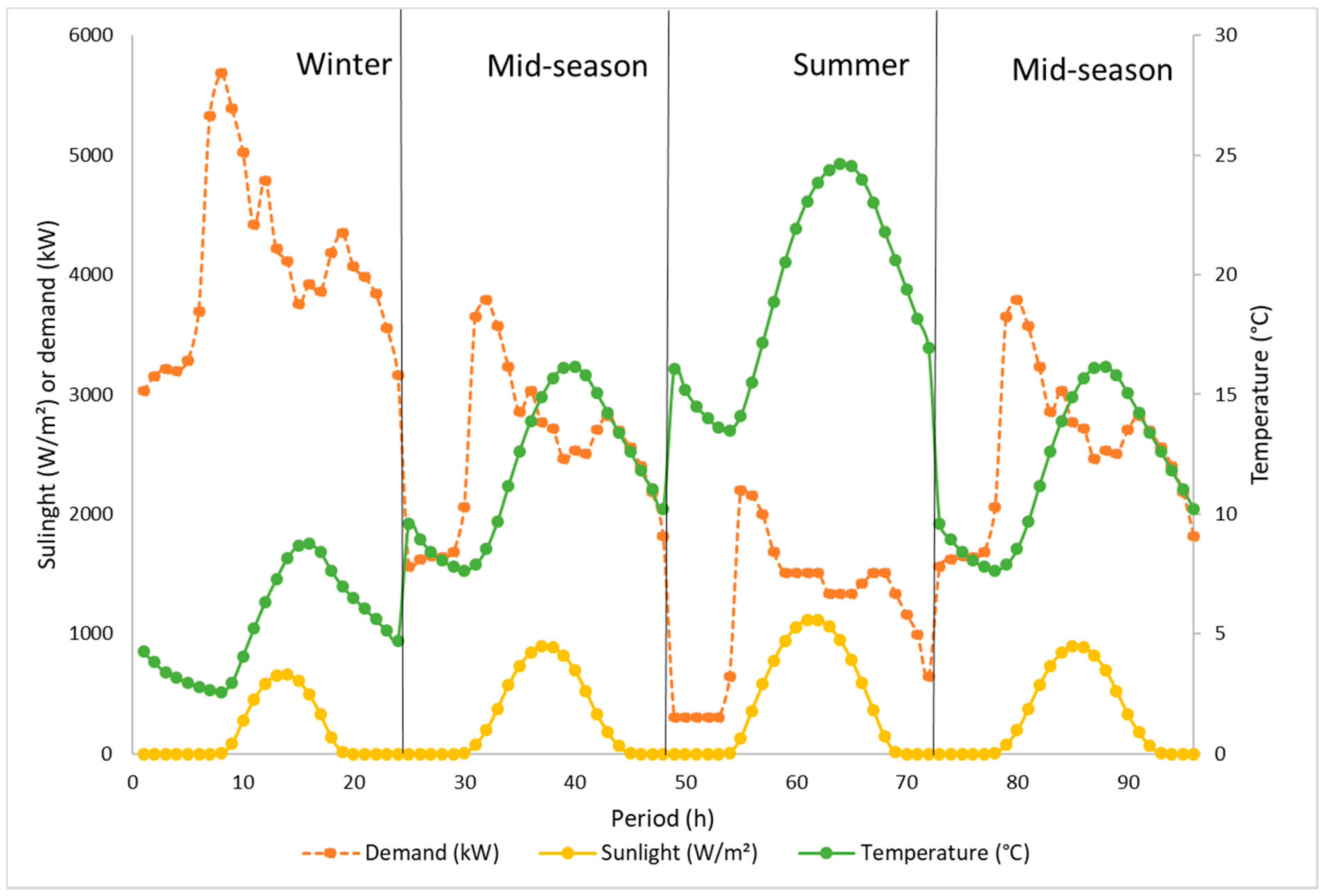
2.1. Creation of Typical Days
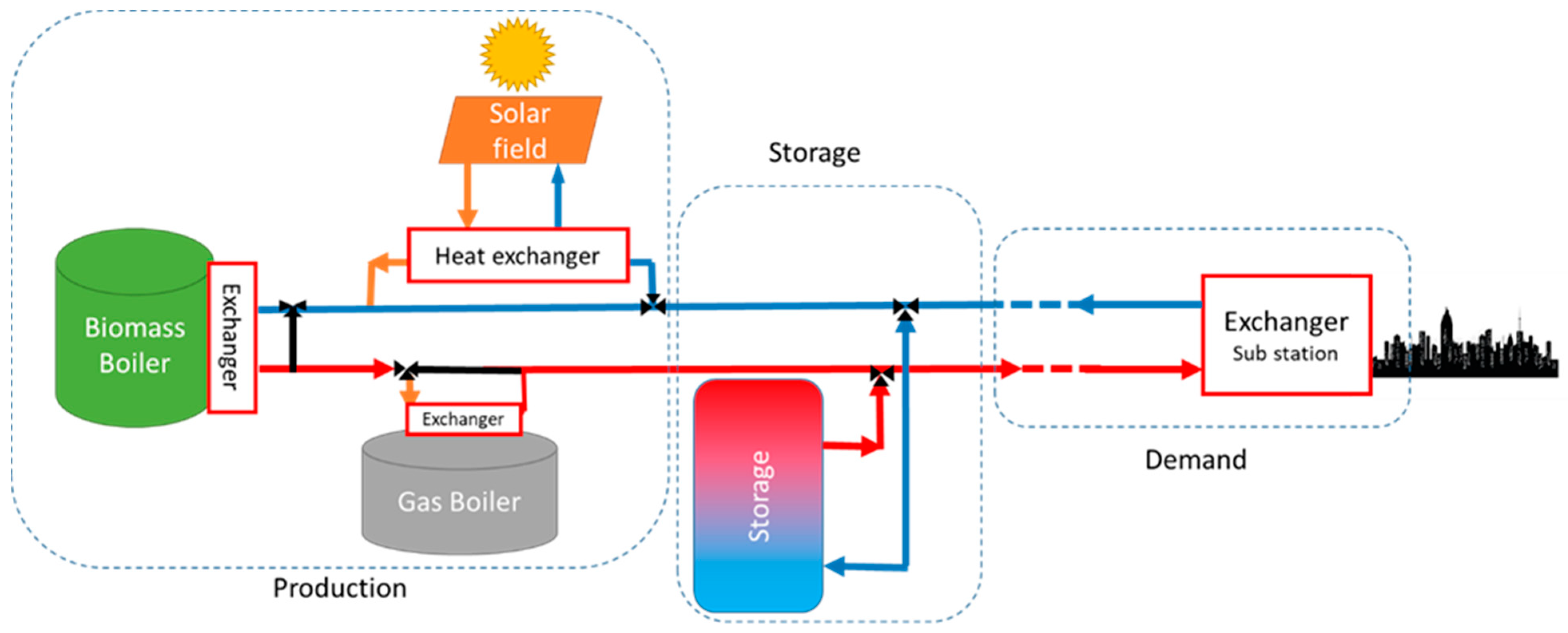
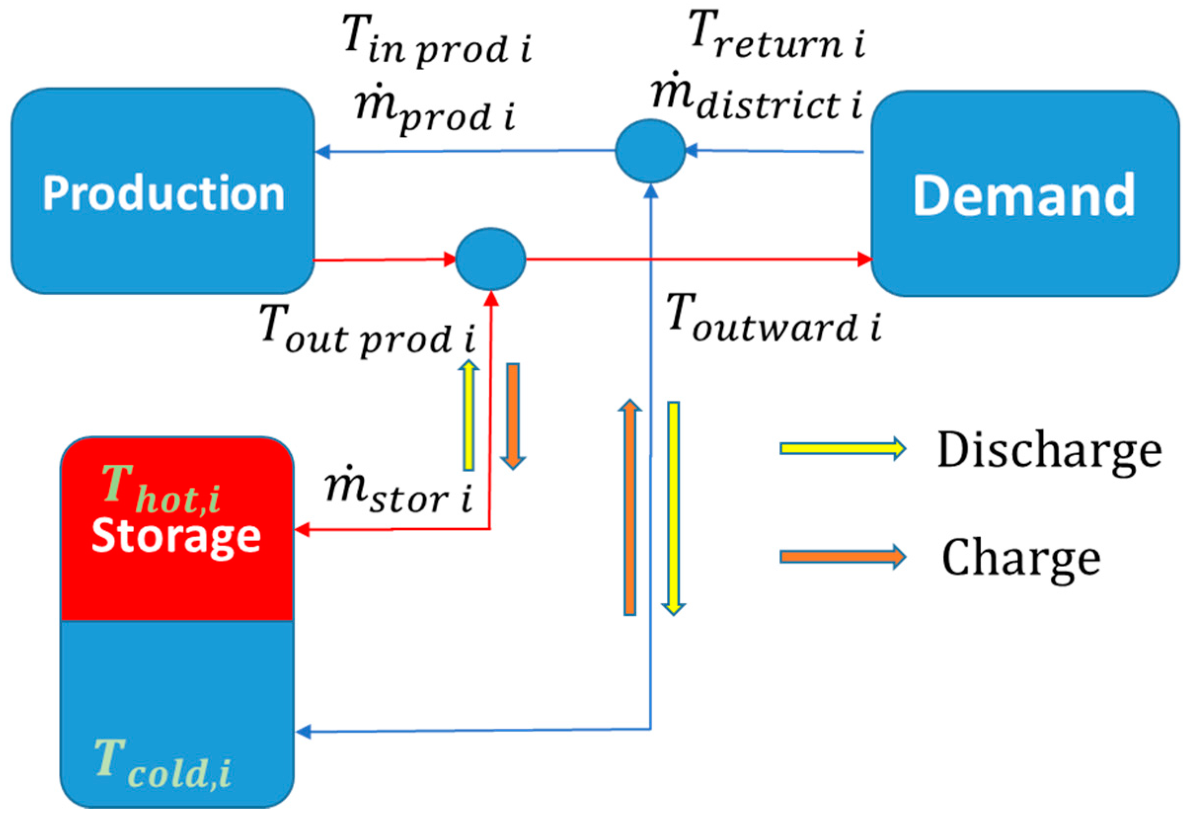
2.2. Model of the DHN
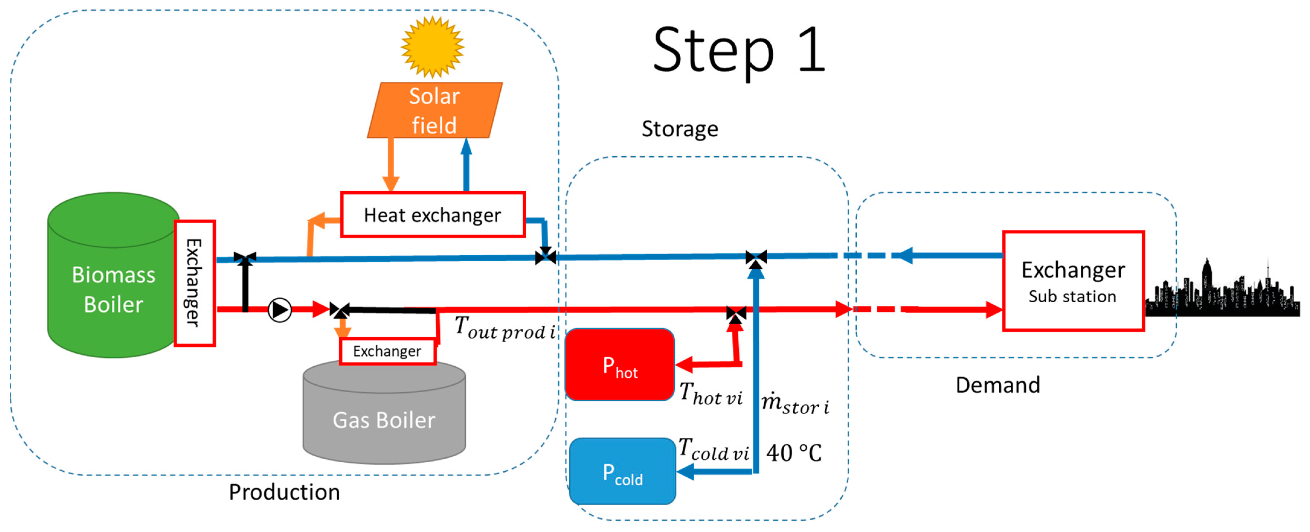
2.3. Model of the Heat Production Systems
2.3.1. Solar Field
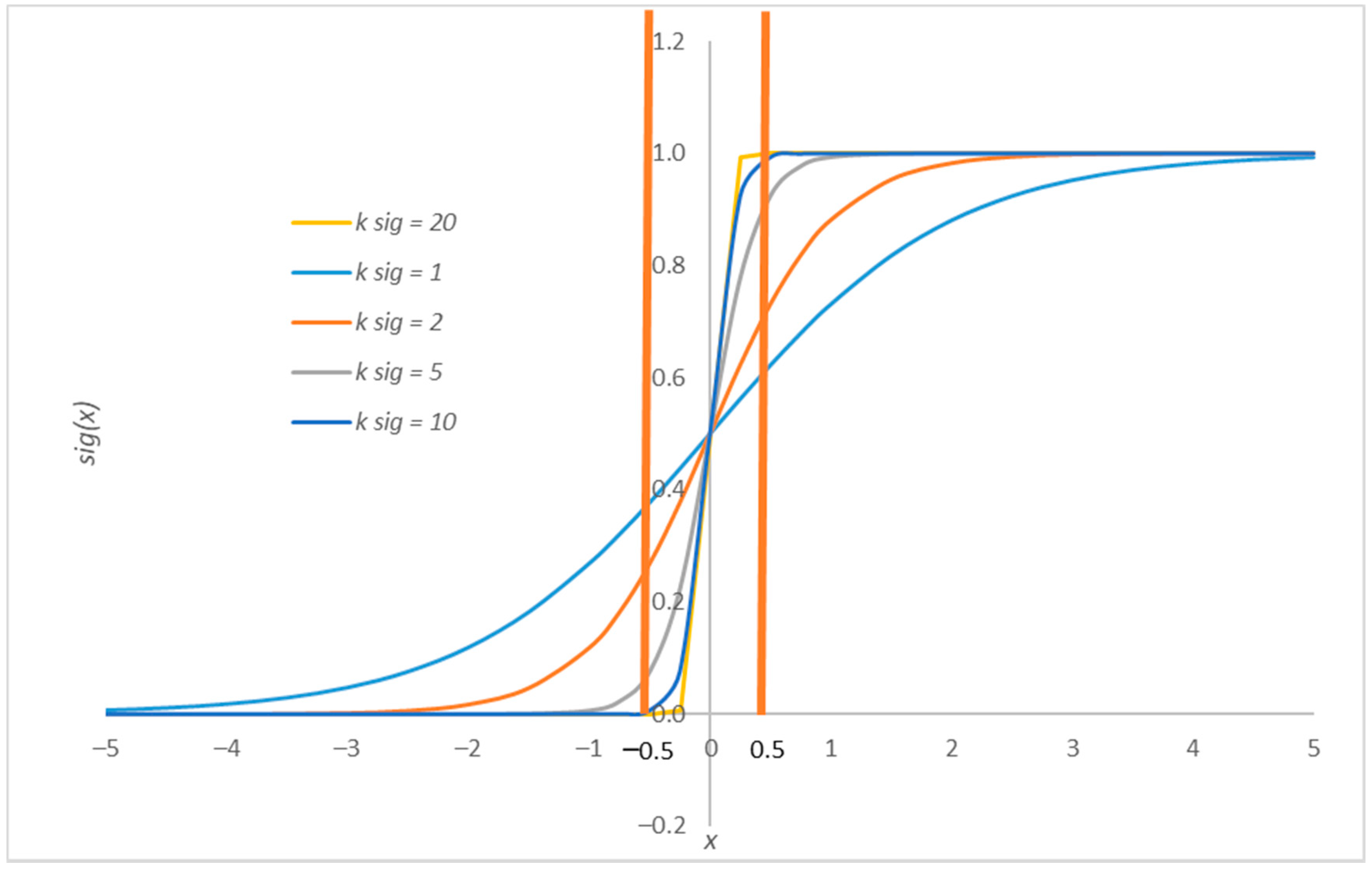
- If the output temperature of the solar field is too low to be able to exchange with the network while respecting the pinch, becomes zero so that Equations (8) and (9) remain verified. In reality, during these periods the output temperature of the solar field can gradually increase. Our model is quasistatic; thus, our modeling leads to , and the solution of Equation (6) leads to an average equilibrium temperature of the field for the considered period.
- If the temperature is high enough, , and are calculated using Equations (6) and (7) and are able to deliver heat to the network provided that the fixed pinch is respected. In this study, the pinch value is set at .
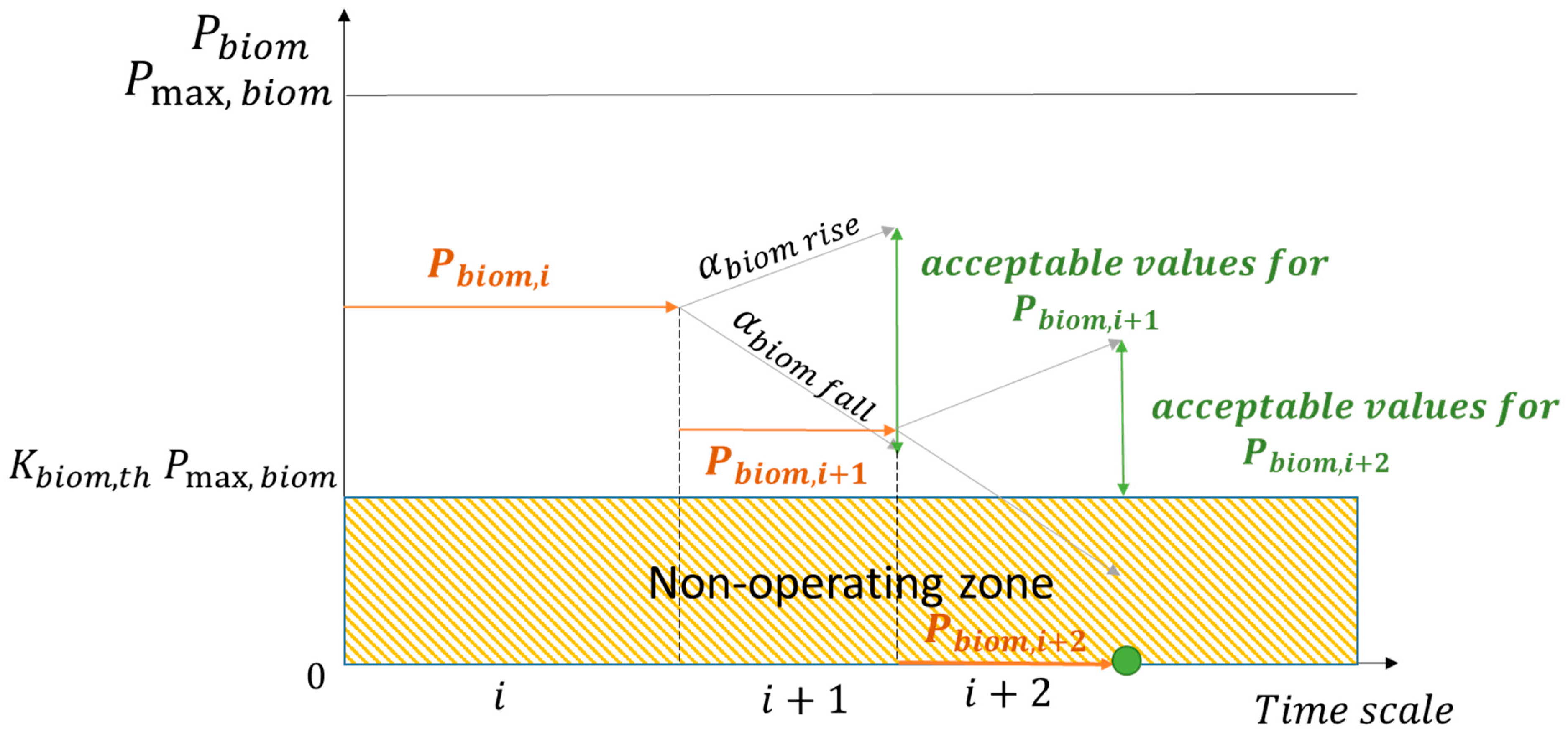
2.3.2. Boilers
- 3
- Two kinds of boiler are modeled: a wood-fueled boiler (called biomass boiler) and a gas boiler. They are modeled by Equations (10)–(12).
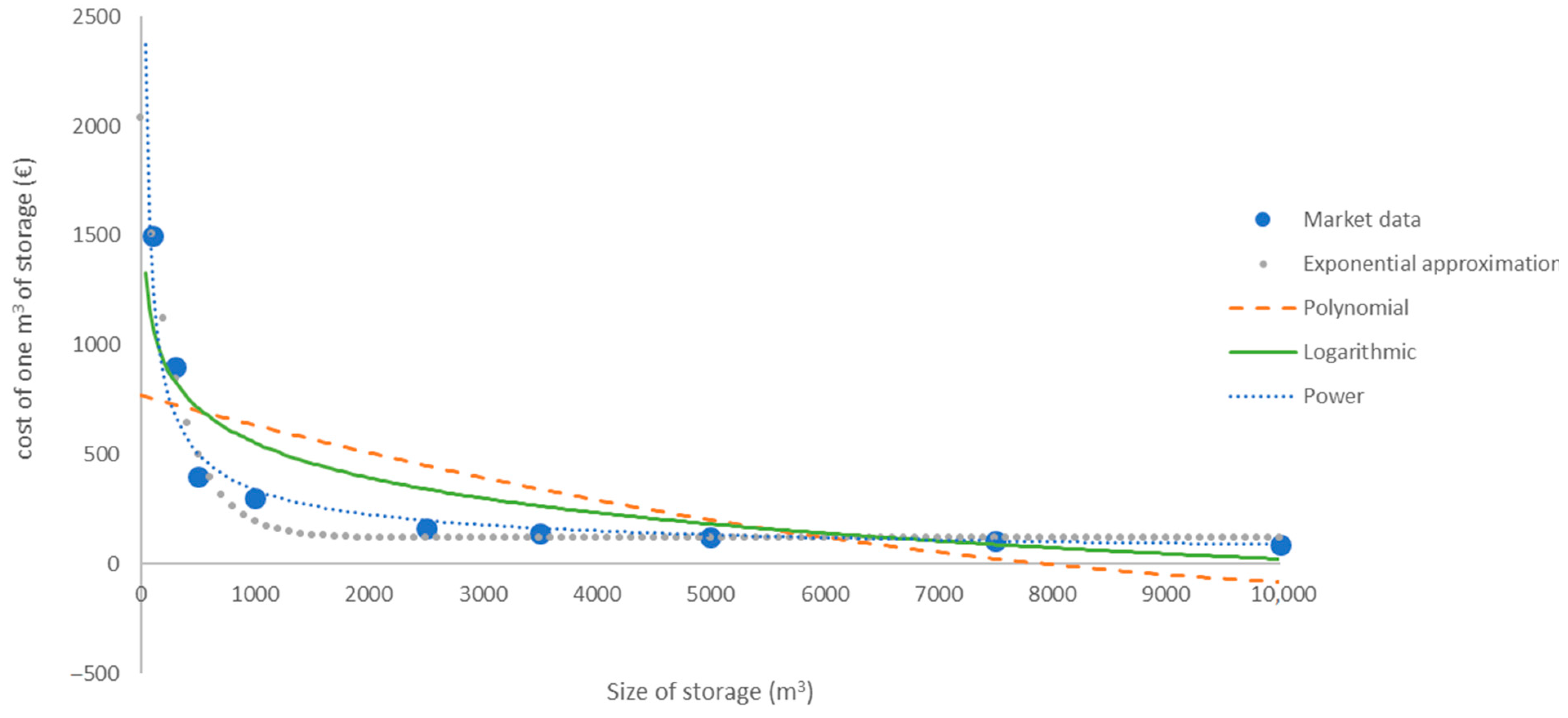
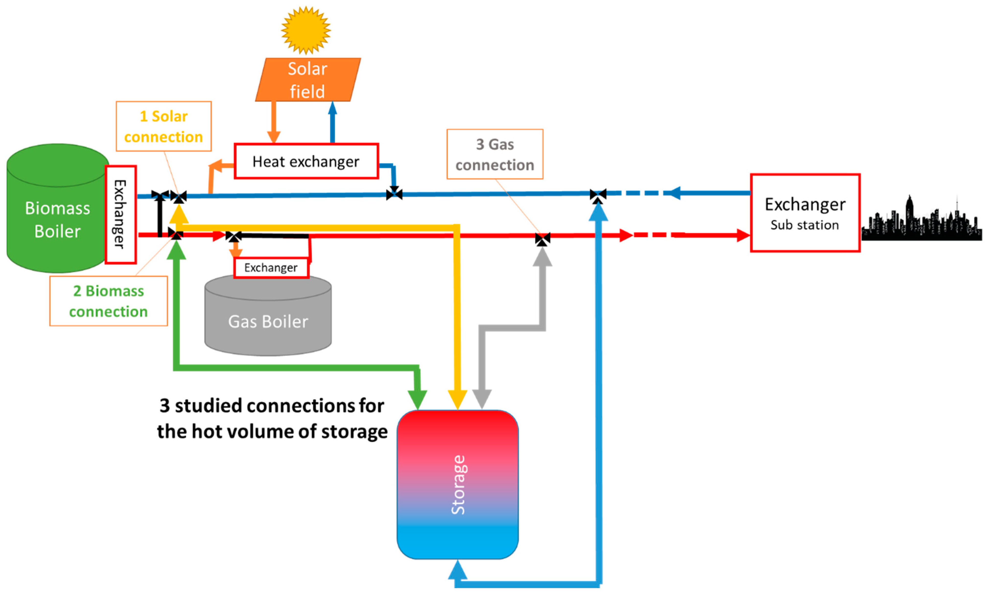
2.4. Storage Model
2.5. Economical Model
- -
- The first part (Equation (34)) covers the use of fuels across all time periods. The cost per unit can vary every year depending on scenarios (here they are constant:, ); nby is the lifespan of the installation. This cost is zero in the case of solar:
- -
- The second part of the operating costs covers light maintenance. This is expressed by Equations (35)–(37) with , , , and :
- -
- The last part of the operating costs covers heavy maintenance, which depends on the size of the installation, represented here by CapEx (, and ):
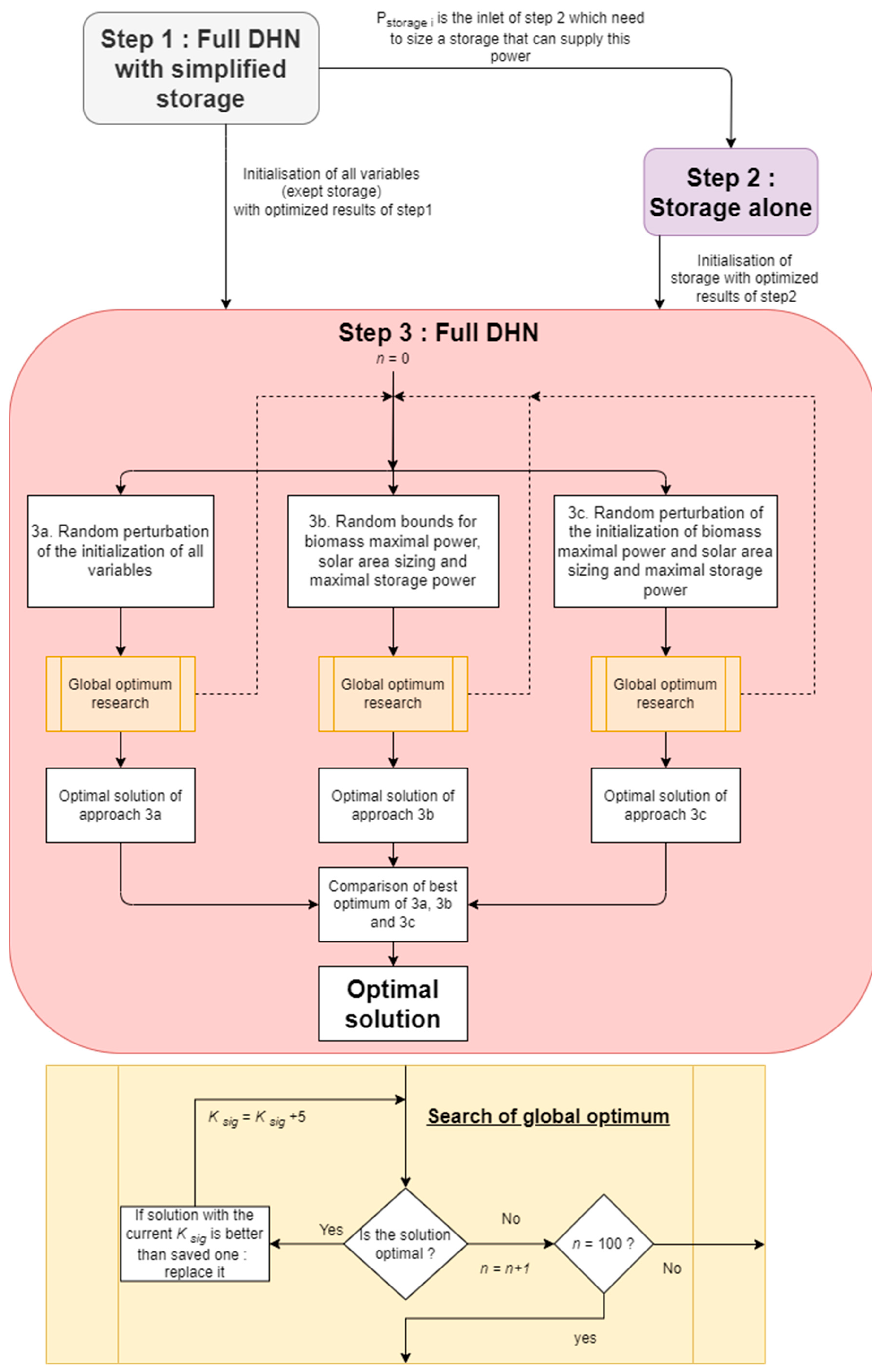
2.6. Resolution Strategy
- Random perturbation to the initialization of all the variables.
- Random perturbation to the bounds of the 3 most sensitive variables:
- Lower bound of the maximum power of the biomass boiler.
- Lower bound of the surface area of the solar field.
- Lower bound of the power that the storage can supply.
- Random perturbation to the initialization of these same 3 sensitive variables.
2.7. Julia (JuMP)
3. Case Study
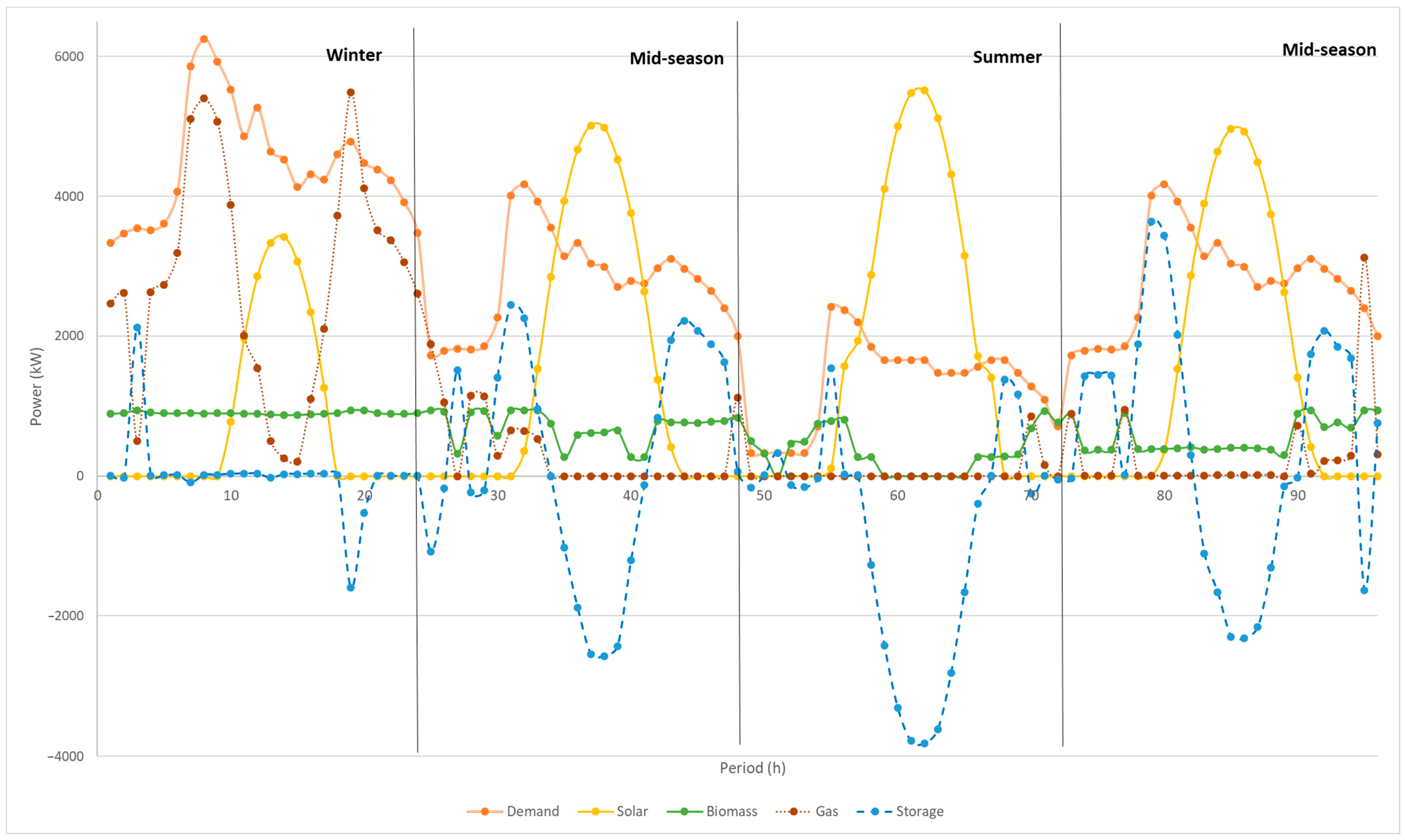
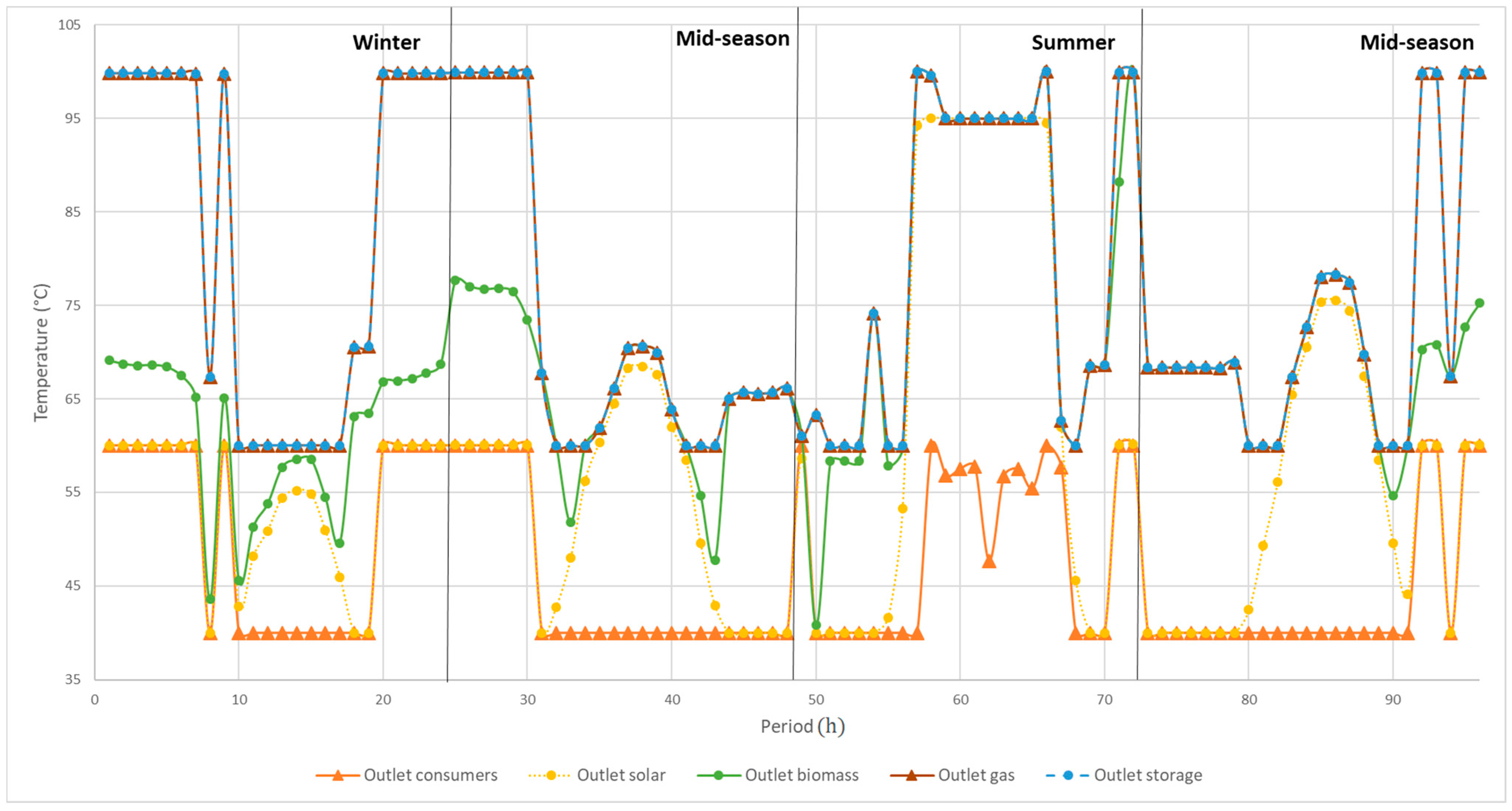
4. Results and Discussion
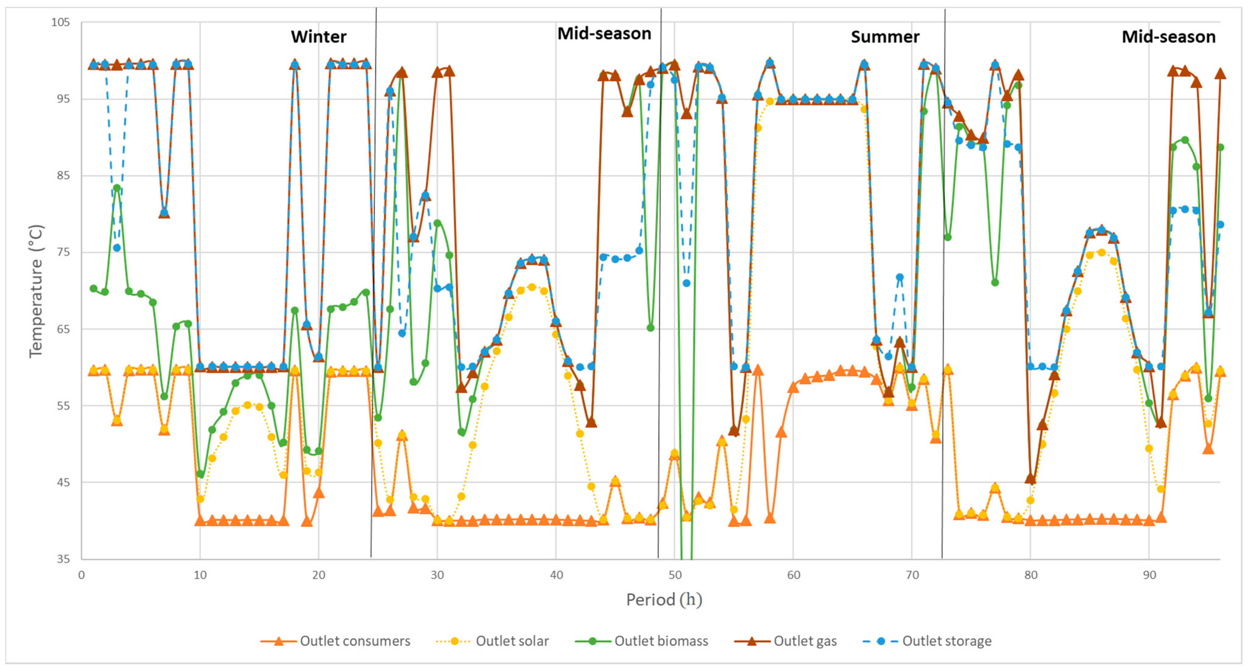
4.1. Results of the Resolution Strategy
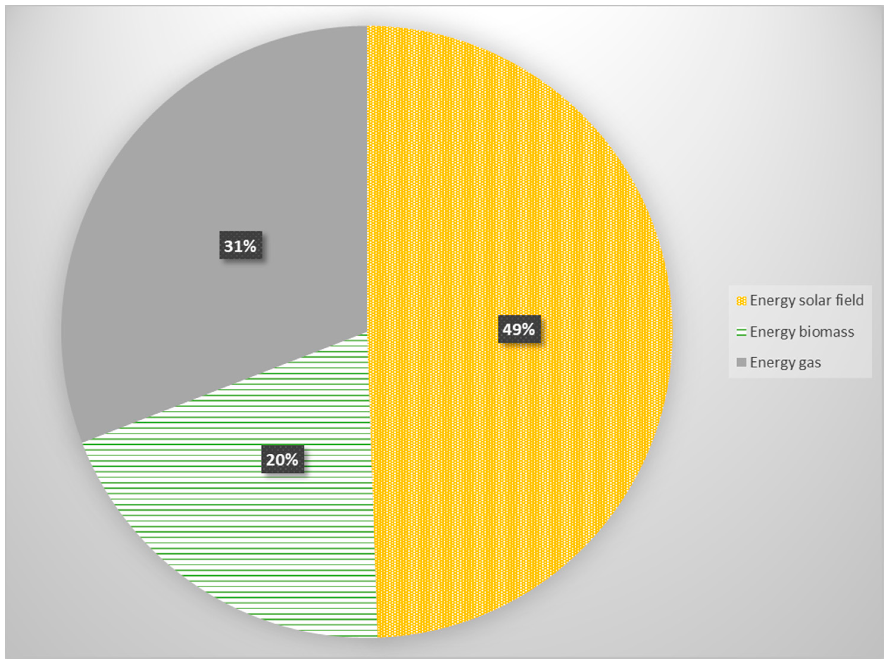
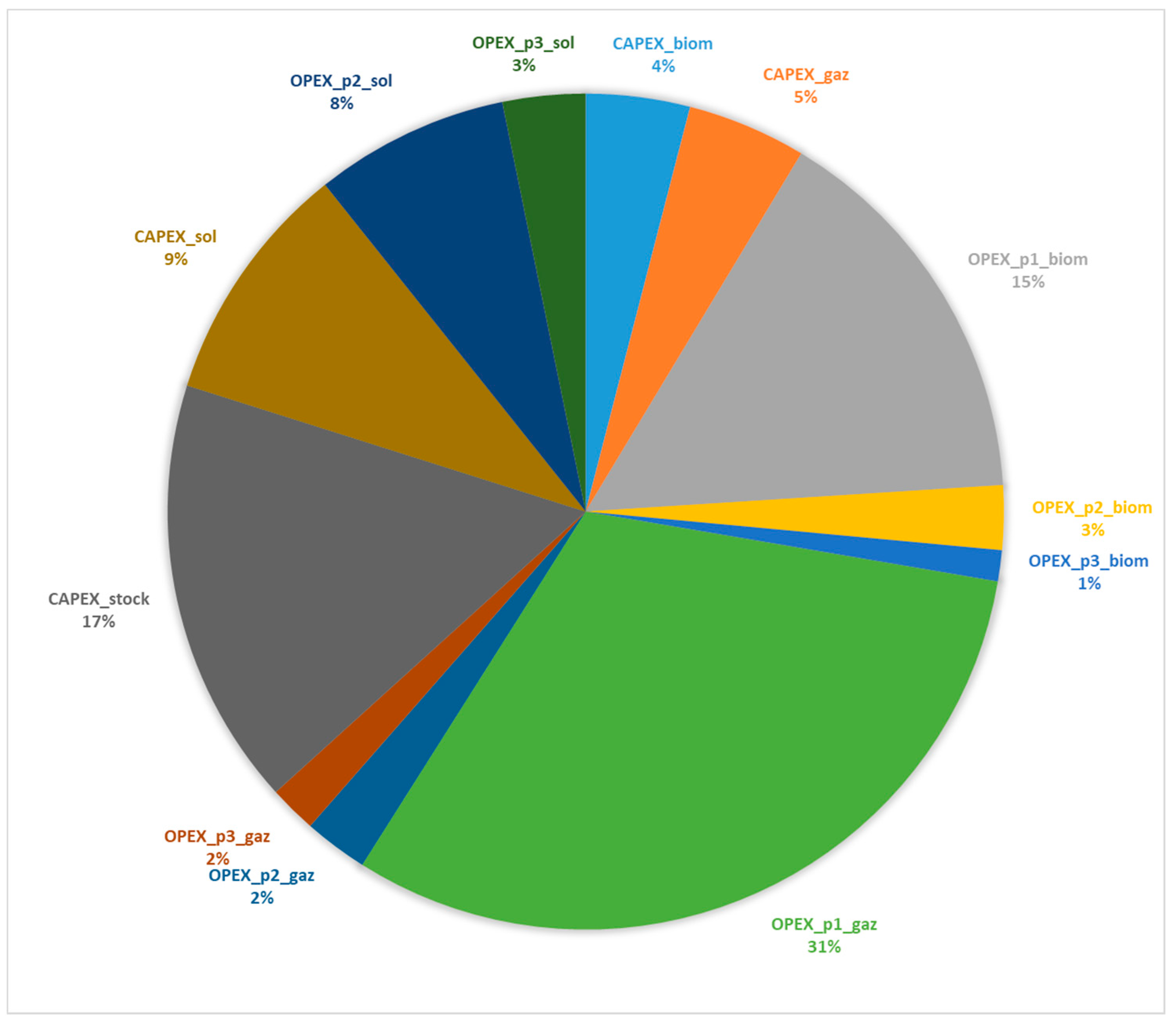
4.2. Study of Different Storage Connections
5. Conclusions
Author Contributions
Funding
Acknowledgments
Conflicts of Interest
Nomenclature
| A | area, m2 |
| a, b, c | coefficients for functions |
| C | product of and , W K−1 |
| specific heat, J kg−1 K−1 | |
| total costs, EUR | |
| E | efficiency |
| global Irradiance, W m−2 | |
| K | using rate of boiler |
| loss factor of storage, s−1 | |
| k | sigmoid coefficient, specific to use |
| mass flow rate, kg s−1 | |
| nby | lifespan, years |
| P | power, W |
| heat transfer, W | |
| T | temperature, °C |
| U | overall heat transfer coefficient, W m−2 K−1 |
| V | volume, m3 |
| y | year |
| Greek symbols | |
| biomass inertia coefficient, W s−2 | |
| first panel coefficient, W m−2 K−1 | |
| second panel coefficient, Wm−2 K−2 | |
| time step between two periods, s | |
| optical yield | |
| efficiency | |
| density, kg m−3 | |
| Subscripts and superscripts | |
| av | average |
| biom | biomass boiler |
| boil | boiler |
| car | characteristic |
| ex | exchanger |
| ext | external |
| i | time step |
| in/out | inlet/outlet |
| min/max | minimum/maximum |
| np | number of periods |
| pan | panel |
| prod | production |
| p1 | operational cost of fuel |
| p2 | operational costs of low maintenance |
| p3 | operational costs of major maintenance |
| sol | solar |
| stor | storage |
| Abbreviations | |
| CapEx | capital expenditure |
| DHN | district heating network |
| HEX | heat exchanger |
| HHV | higher heating value |
| NLP | nonlinear programming |
| NTU | number of transferred units |
| LHV | low heating value |
| OpEx | operational expenditure |
| SDHN | solar district heating network |
| Seas | season |
| Sig | sigmoid function |
References
- Dussud, F.-X.; Guggemos, F.; Riedinger, N. “Chiffres clés de L’énergie Edition 2018.” Service de la Donnée et des études Statistiques (SDES). 2018. Available online: http://reseaux-chaleur.cerema.fr/les-chiffres-cles-de-lenergie-edition-2018 (accessed on 20 October 2021).
- ADEME (Agence de la Transition écologique). Se Chauffer Mieux Et Moins Cher; ADEME: Paris, France, 2014; p. 19. [Google Scholar]
- Lund, H.; Werner, S.; Wiltshire, R.; Svendsen, S.; Thorsen, J.E.; Hvelplund, F.; Mathiesen, B.V. 4th Generation District Heating (4GDH): Integrating smart thermal grids into future sustainable energy systems. Energy 2014, 68, 1–11. [Google Scholar] [CrossRef]
- Mazhar, A.R.; Liu, S.; Shukla, A. A state of art review on the district heating systems. Renew. Sustain. Energy Rev. 2018, 96, 420–439. [Google Scholar] [CrossRef]
- Lake, A.; Rezaie, B.; Beyerlein, S. Review of district heating and cooling systems for a sustainable future. Renew. Sustain. Energy Rev. 2017, 67, 417–425. [Google Scholar] [CrossRef]
- Sameti, M.; Haghighat, F. Optimization approaches in district heating and cooling thermal network. Energy Build. 2017, 140, 121–130. [Google Scholar] [CrossRef]
- Werner, S. International review of district heating and cooling. Energy 2017, 137, 617–631. [Google Scholar] [CrossRef]
- Wiltshire, R. Advanced District Heating and Cooling (DHC) Systems; Woodhead Publishing: London, UK, 2015. [Google Scholar]
- Faninger, G. Combined solar–biomass district heating in Austria. Sol. Energy 2000, 69, 425–435. [Google Scholar] [CrossRef]
- IEA TASK 55. Available online: https://task55.iea-shc.org/about (accessed on 25 October 2021).
- Gao, L.; Hwang, Y.; Cao, T. An overview of optimization technologies applied in combined cooling, heating and power systems. Renew. Sustain. Energy Rev. 2019, 114, 109344. [Google Scholar] [CrossRef]
- Wang, Y.; Zhang, S.; Chow, D.; Kuckelkorn, J.M. Evaluation and optimization of district energy network performance: Present and future. Renew. Sustain. Energy Rev. 2021, 139, 110577. [Google Scholar] [CrossRef]
- Mertz, T.; Serra, S.; Henon, A.; Reneaume, J.-M. A MINLP optimization of the configuration and the design of a district heating network: Academic study cases. Energy 2016, 117, 450–464. [Google Scholar] [CrossRef]
- Marty, F.; Serra, S.; Sochard, S.; Reneaume, J.-M. Economic optimization of a combined heat and power plant: Heat vs electricity. Energy Procedia 2017, 116, 138–151. [Google Scholar] [CrossRef]
- Marty, F.; Serra, S.; Sochard, S.; Reneaume, J.-M. Exergy Analysis and Optimization of a Combined Heat and Power Geothermal Plant. Energies 2019, 12, 1175. [Google Scholar] [CrossRef] [Green Version]
- Marty, F.; Sochard, S.; Serra, S.; Reneaume, J.-M. Multi-objective approach for a combined heat and power geothermal plant optimization. Chem. Prod. Process Model. 2020, 16, 20200008. [Google Scholar] [CrossRef]
- Powell, K.M.; Edgar, T.F. Modeling and control of a solar thermal power plant with thermal energy storage. Chem. Eng. Sci. 2012, 71, 138–145. [Google Scholar] [CrossRef]
- Powell, K.M.; Cole, W.J.; Ekarika, U.F.; Edgar, T.F. Dynamic optimization of a campus cooling system with thermal storage. In Proceedings of the 2013 European Control Conference (ECC), Zurich, The Netherlands, 17–19 July 2013; pp. 4077–4082. [Google Scholar]
- Powell, K.M.; Hedengren, J.D.; Edgar, T.F. Dynamic optimization of a hybrid solar thermal and fossil fuel system. Sol. Energy 2014, 108, 210–218. [Google Scholar] [CrossRef]
- Scolan, S. Dynamic optimization of the operation of a solar thermal plant. Sol. Energy 2020, 198, 643–657. [Google Scholar] [CrossRef]
- Nova-Rincon, A.; Sochard, S.; Serra, S.; Reneaume, J.-M. Dynamic simulation and optimal operation of district cooling networks via 2D orthogonal collocation. Energy Convers. Manag. 2020, 207, 112505. [Google Scholar] [CrossRef]
- Suciu, R.; Kantor, I.; Bütün, H.; Maréchal, F. Geographically Parameterized Residential Sector Energy and Service Profile. Front. Energy Res. 2019, 7, 69. [Google Scholar] [CrossRef] [Green Version]
- Casisi, M.; Pinamonti, P.; Reini, M. Optimal lay-out and operation of combined heat & power (CHP) distributed generation systems. Energy 2009, 34, 2175–2183. [Google Scholar] [CrossRef]
- Elsido, C.; Martelli, E.; Grossmann, I.E. Multiperiod optimization of heat exchanger networks with integrated thermodynamic cycles and thermal storages. Comput. Chem. Eng. 2021, 149, 107293. [Google Scholar] [CrossRef]
- Kim, J.H.; Han, C. Short-Term Multiperiod Optimal Planning of Utility Systems Using Heuristics and Dynamic Programming. Ind. Eng. Chem. Res. 2001, 40, 1928–1938. [Google Scholar] [CrossRef]
- Morvaj, B.; Evins, R.; Carmeliet, J. Optimising urban energy systems: Simultaneous system sizing, operation and district heating network layout. Energy 2016, 116, 619–636. [Google Scholar] [CrossRef]
- Carpaneto, E.; Lazzeroni, P.; Repetto, M. Optimal integration of solar energy in a district heating network. Renew. Energy 2015, 75, 714–721. [Google Scholar] [CrossRef]
- Buoro, D.; Pinamonti, P.; Reini, M. Optimization of a Distributed Cogeneration System with solar district heating. Appl. Energy 2014, 124, 298–308. [Google Scholar] [CrossRef]
- Casisi, M.; Buoro, D.; Pinamonti, P.; Reini, M. A Comparison of Different District Integration for a Distributed Generation System for Heating and Cooling in an Urban Area. Appl. Sci. 2019, 9, 3521. [Google Scholar] [CrossRef] [Green Version]
- Grossmann, I.E. Mixed-Integer Optimization Techniques for Algorithmic Process Synthesis. In Advances in Chemical Engineering; Elsevier: Amsterdam, The Netherlands, 1996; Volume 23, pp. 171–246. ISBN 978-0-12-008523-1. [Google Scholar]
- Biegler, L.T.; Grossmann, I.E. Retrospective on optimization. Comput. Chem. Eng. 2004, 28, 1169–1192. [Google Scholar] [CrossRef]
- Connolly, D.; Lund, H.; Mathiesen, B.V.; Leahy, M. A review of computer tools for analysing the integration of renewable energy into various energy systems. Appl. Energy 2010, 87, 1059–1082. [Google Scholar] [CrossRef]
- Limpens, G.; Moret, S.; Jeanmart, H.; Maréchal, F. EnergyScope TD: A novel open-source model for regional energy systems. Appl. Energy 2019, 255, 113729. [Google Scholar] [CrossRef]
- Limpens, G.; Jeanmart, H.; Maréchal, F. Belgian Energy Transition: What Are the Options? Energies 2020, 13, 261. [Google Scholar] [CrossRef] [Green Version]
- Welcome|TRNSYS: Transient System Simulation Tool. Available online: http://www.trnsys.com/index.html (accessed on 4 December 2019).
- Østergaard, P.A. Reviewing EnergyPLAN simulations and performance indicator applications in EnergyPLAN simulations. Appl. Energy 2015, 154, 921–933. [Google Scholar] [CrossRef]
- Openmod—Open Energy Modelling Initiative. Available online: https://www.openmod-initiative.org/ (accessed on 4 December 2019).
- Bezanson, J.; Karpinski, S.; Shah, V.; Edelman, A. The Julia Language. Available online: https://julialang.org/ (accessed on 12 December 2019).
- Dunning, I.; Huchette, J.; Lubin, M. JuMP: A Modeling Language for Mathematical Optimization. SIAM Rev. 2017, 59, 295–320. [Google Scholar] [CrossRef]
- Åberg, M.; Widén, J. Development, validation and application of a fixed district heating model structure that requires small amounts of input data. Energy Convers. Manag. 2013, 75, 74–85. [Google Scholar] [CrossRef]
- Vesterlund, M.; Dahl, J. A method for the simulation and optimization of district heating systems with meshed networks. Energy Convers. Manag. 2015, 89, 555–567. [Google Scholar] [CrossRef]
- Pfenninger, S. Dealing with multiple decades of hourly wind and PV time series in energy models: A comparison of methods to reduce time resolution and the planning implications of inter-annual variability. Appl. Energy 2017, 197, 1–13. [Google Scholar] [CrossRef]
- Kotzur, L. Time series aggregation for energy system design_ Modeling seasonal storage. Appl. Energy 2018, 213, 123–135. [Google Scholar] [CrossRef] [Green Version]
- Domínguez-Muñoz, F.; Cejudo-López, J.M.; Carrillo-Andrés, A.; Gallardo-Salazar, M. Selection of typical demand days for CHP optimization. Energy Build. 2011, 43, 3036–3043. [Google Scholar] [CrossRef]
- Lozano, M.A.; Anastasia, A.; Serra, L.M.; Verda, V. Thermoeconomic Cost Analysis of Central Solar Heating Plants Combined With Seasonal Storage. In Proceedings of the ASME 2010 International Mechanical Engineering Congress and Exposition, Vancouver, BC, Canada, 12–18 November 2010; pp. 643–653. [Google Scholar]
- Sartor, K.; Quoilin, S.; Dewallef, P. Simulation and optimization of a CHP biomass plant and district heating network. Appl. Energy 2014, 130, 474–483. [Google Scholar] [CrossRef] [Green Version]
- Loo, S.; van Koppejan, J. The Handbook of Biomass Combustion and Co-Firing; Earthscan: London, UK, 2008. [Google Scholar]
- Roos, P.; Haselbacher, A. Thermocline control through multi-tank thermal-energy storage systems. Appl. Energy 2021, 281, 115971. [Google Scholar] [CrossRef]
- van der Heijde, B.; Vandermeulen, A.; Salenbien, R.; Helsen, L. Representative days selection for district energy system optimisation: A solar district heating system with seasonal storage. Appl. Energy 2019, 248, 79–94. [Google Scholar] [CrossRef]
- Solar District Heating. Available online: https://www.solar-district-heating.eu/en/plant-database/ (accessed on 20 October 2021).


| Approach | Solar Area (m2) | Storage Size (m3) | Total Costs (Million EUR) | |
|---|---|---|---|---|
| a | 5707 | 20,068 | 2265 | 24.931 |
| b | 7749 | 35,006 | 1137 | 24.811 |
| c | 4500 | 12,159 | 2221 | 25.333 |
| Approach | Convergence (%) | Average Total Costs (Million EUR) | Standard Deviation | Calculation Time |
|---|---|---|---|---|
| a | 3 | 25.040 | 0.0770 | 3 h 43 min |
| b | 20 | 25.759 | 0.5611 | 3 h 49 min |
| c | 5 | 25.420 | 0.0627 | 3 h 48 min |
| Connection | Total Costs (Million EUR) | ||||
|---|---|---|---|---|---|
| 1—Solar | b. 10 | 24.348 | 7812 | 916.3 | 35,209 |
| 2—Biomass | a. 10 | 24.975 | 6576 | 983.7 | 26,516 |
| 3—Gas | b. 10 | 24.811 | 7749 | 1137 | 35,006 |
Publisher’s Note: MDPI stays neutral with regard to jurisdictional claims in published maps and institutional affiliations. |
© 2021 by the authors. Licensee MDPI, Basel, Switzerland. This article is an open access article distributed under the terms and conditions of the Creative Commons Attribution (CC BY) license (https://creativecommons.org/licenses/by/4.0/).
Share and Cite
Delubac, R.; Serra, S.; Sochard, S.; Reneaume, J.-M. A Dynamic Optimization Tool to Size and Operate Solar Thermal District Heating Networks Production Plants. Energies 2021, 14, 8003. https://doi.org/10.3390/en14238003
Delubac R, Serra S, Sochard S, Reneaume J-M. A Dynamic Optimization Tool to Size and Operate Solar Thermal District Heating Networks Production Plants. Energies. 2021; 14(23):8003. https://doi.org/10.3390/en14238003
Chicago/Turabian StyleDelubac, Régis, Sylvain Serra, Sabine Sochard, and Jean-Michel Reneaume. 2021. "A Dynamic Optimization Tool to Size and Operate Solar Thermal District Heating Networks Production Plants" Energies 14, no. 23: 8003. https://doi.org/10.3390/en14238003
APA StyleDelubac, R., Serra, S., Sochard, S., & Reneaume, J.-M. (2021). A Dynamic Optimization Tool to Size and Operate Solar Thermal District Heating Networks Production Plants. Energies, 14(23), 8003. https://doi.org/10.3390/en14238003