Article

Short-Term Forecasting of Wind Energy: A Comparison of Deep Learning Frameworks

1
Department of Statistics, Universidad Carlos III de Madrid, 28903 Getafe, Spain
2
ICADE, Department of Quantitative Methods, Faculty of Economics and Business Administration, Universidad Pontificia Comillas, 28015 Madrid, Spain
3
Institute for Research in Technology (IIT), ICAI School of Engineering, Universidad Pontificia Comillas, 28015 Madrid, Spain
*
Author to whom correspondence should be addressed.
Energies 2021, 14(23), 7943; https://doi.org/10.3390/en14237943
Submission received: 30 September 2021 / Revised: 4 November 2021 / Accepted: 22 November 2021 / Published: 26 November 2021

Abstract

:
Wind energy has been recognized as the most promising and economical renewable energy source, attracting increasing attention in recent years. However, considering the variability and uncertainty of wind energy, accurate forecasting is crucial to propel high levels of wind energy penetration within electricity markets. In this paper, a comparative framework is proposed where a suite of long short-term memory (LSTM) recurrent neural networks (RNN) models, inclusive of standard, bidirectional, stacked, convolutional, and autoencoder architectures, are implemented to address the existing gaps and limitations of reported wind power forecasting methodologies. These integrated networks are implemented through an iterative process of varying hyperparameters to better assess their effect, and the overall performance of each architecture, when tackling one-hour to three-hours ahead wind power forecasting. The corresponding validation is carried out through hourly wind power data from the Spanish electricity market, collected between 2014 and 2020. The proposed comparative error analysis shows that, overall, the models tend to showcase low error variability and better performance when the networks are able to learn in weekly sequences. The model with the best performance in forecasting one-hour ahead wind power is the stacked LSTM, implemented with weekly learning input sequences, with an average MAPE improvement of roughly 6, 7, and 49%, when compared to standard, bidirectional, and convolutional LSTM models, respectively. In the case of two to three-hours ahead forecasting, the model with the best overall performance is the bidirectional LSTM implemented with weekly learning input sequences, showcasing an average improved MAPE performance from 2 to 23% when compared to the other LSTM architectures implemented.

1. Introduction

The rising concerns over global warming, energy security, and the impact of Greenhouse gas (GHG) emissions on the global economy have increased interest in developing efficient renewable energy sources for the rapid replacement of fossil fuels [1]. Governments around the world have stepped up their climate ambitions. By the end of 2020, 28 countries had issued “climate emergency” declarations, many of which were accompanied by plans and targets to transition to more renewable-based energy systems [2]. Wind power has emerged as the most promising and economical renewable energy source. The global wind power market expanded 19% in 2019 to 60 GW, for a total global capacity of 650 GW (621 GW onshore and the rest offshore) [2]. While economic factors are the driving force for the steady growth of wind power, the variability and uncertainty of wind energy pose challenges in the operation, scheduling, and planning of power systems, which ultimately increase generation costs [3]. Therefore, accurate forecasting is crucial for wind power generation systems and to propel high levels of wind energy penetration.
According to schedulers, dispatchers, and energy planners, among the most important was the need for a day-ahead wind power forecast for energy trading and the unit commitment schedule, followed by hourly forecasts (expressed in megawatts) inclusive of error bars and uncertainty intervals, and forecasts several days ahead for maintenance planning [4]. In order to meet these demands, numerous forecasting studies have been carried out focusing on wind speed and power forecasting, uncertainty forecasting, and ramp events forecasting in different time horizons [5,6]. Throughout the years, wind energy forecasting has been tackled through different approaches such as physical or numerical weather prediction (NWP) models, statistical and probabilistic methods, intelligent forecasting models, and hybrid or ensemble methods. These models are mainly carried through four forecasting time horizons: very-short term (<30 min), short term (0.5–6 h), medium term (6–24 h), and long term (1–7 days) [7].
The physical method uses physical and weather information, such as wind direction, roughness, obstruction, pressure, and temperature, to model wind power. Due to its high dependence on numerical weather forecast data, accuracy is greatly affected by the precision of numerical weather predictions [8]. On the other hand, statistical methods are mainly based on historical data, focusing on the time-varying relationships of given time sequences, often requiring high model orders to describe the linear relationship of wind series. Some traditional statistical models are the Kalman filter (KF) and the autoregressive integrated moving average model (ARIMA) [9]. However, in recent literature, research has moved towards the implementation of machine learning (ML) methods, mainly due to the performance of such models in extracting robust features, which have reported huge success in a wide range of applications [10,11]. ML models, such as artificial neural networks (ANN) [12] and support vector machines (SVM) [13], can establish a nonlinear mapping to accurately describe wind randomness. In this line of thought, in [14], wind speed and wind power output are predicted in the short term by means of a group method of data handling (GMDH)-neural network approach. Although this approach has presented interesting results, some drawbacks have been reported. Specifically, the model tends to produce an exceedingly complex network when it comes to highly nonlinear systems due to its limited generic structure (quadratic two-variable polynomial) [15]. In order to obtain higher accuracy values, SVM-based models have been proposed. For instance, in [16], a hybrid model (LSSVM–GSA) based on the least squares support vector machine (LSSVM) and gravitational search algorithm (GSA) has been proposed to forecast the short-term wind power. For these kinds of approaches, it has been reported that they usually involve a very complex optimization process [17].
While ML and hybrid models may better capture the nonlinear dynamics of renewable energy generation processes, most models are non-trivial to tune and use in practice. They depend on careful selection of input features and pre-treatment strategies and have difficulties dealing with vanishing or exploding gradients [18]. Due to the limitations and poor adaptability of traditional ML models, deep learning (DL) methods have been applied to wind power forecasting. Recurrent neural networks (RNN) have been especially highlighted to model the relationships among samples of time sequences. In this way, the use of gates in recurrent units (long short-term memory (LSTM), gated recurrent units (GRUs), among others) has successfully increased the accuracy of results in forecasting tasks. GRU and LSTM both use different ways of gating information to prevent vanishing gradient problems. In the first case, the GRU has two gates to model time dependencies that are reset and update gates, while LSTM has three gates that are input, output, and forget. In this way, the GRU controls the flow of information like the LSTM unit, but without having to use a memory unit. As advantages, the GRU uses less training parameters and, therefore, uses less memory, executes faster, and trains faster than LSTM, whereas LSTM is more accurate on a dataset using longer sequences. In short, it has been proved in different applications that if sequences are large or accuracy is very critical, LSTM performance is preferred, whereas GRU is selected in some classification tasks where less memory consumption and faster operation is required [19,20,21]. For this reason, as will be seen, most of the state-of-the-art research in wind power forecasting, using deep learning, involves the LSTM approach.
In the literature, different wind power forecasting strategies have been developed by implementing diverse LSTM models. In [22], medium-term wind power forecasting was performed using LSTM networks on historical wind power data and NWP data. In this case, the latter data type was first analyzed by principal component analysis (PCA) to narrow down the meteorological inputs. The study produced similar results for both LSTM and PCA-LSTM results; however, the latter hybrid model slightly outperformed the LSTM, yet both proved to be superior when compared to SVM models and backpropagation (BP) neural networks performance metrics. In [23], short-term wind power forecasting was developed, for one to five steps ahead, based on discrete wavelet transform (DWT) and LSTM networks. DWT decomposed original wind power data from three different wind farms into low-frequency and high-frequency sub-signals, such that independent LSTMs approximate the temporal dynamic behaviors of the sub-signals, respectively. The proposed DWT LSTM model proved to perform better when compared to RNN and BP methods alone; however, when steps ahead increased, the performance metrics deteriorated. In [24], a combined model consisting of the variational mode decomposition (VMD), convolutional LSTM network (ConvLSTM), and error analysis was conducted for short-term wind power forecasting. The proposed VMD-ConvLSTM-LSTM model was implemented on historical output data series from two wind turbines and two wind farms. The proposed model proved to outperform traditional forecasting algorithms; however, model parameters were selected by expertise given the large computational cost associated with the estimation of optimal parameters.
Additional strategies have been implemented in related research areas, such as the wind speed forecasting field. In [25], a model combining ARIMA and dynamic evolving neural-fuzzy inference system (DENFIS) for wind speed forecasting has been proposed, reporting RMSE values of 0.07 and 0.13 for 2 and 6 hour ahead forecasting, respectively. As a reported drawback, DENFIS needs prior assumptions about data and requires domain knowledge to define the associated parameters [26]. Other ML-based models have been proposed to improve the forecasting accuracy. Specifically, in [27], a hybrid approach based on the CRO (coral reefs optimization) algorithm and the extreme learning machine (ELM) is presented. The CRO was implemented to reduce the number of variables and the ELM was used to provide the wind speed prediction. The main limitation of this approach is that the performance is very unstable. It is very difficult to find the best parameters such that the training and testing accuracy is maximum for a given problem [28]. In order to improve the error/accuracy metrics, DL-based models have been proposed.
In particular, in [29], a multivariate stacked LSTM model is proposed. Historical wind speed, wind direction, temperature, humidity, pressure, dew point, and solar radiation are used to predict future short-term wind speed. The study proposes a model with two LSTM layers stacked after the input layer, with 64 neurons each. The results proved to outperform multiple competing statistical methods, including multiple linear regression, LASSO, and ridge-based strategies. In the same line, in [30], a hybrid particle swarm optimization–ant lion optimizer (hPSO–ALO) was used for training the weight values of LSTM network. However, limitations associated to ALO-based algorithms are related to the long run time due to the random ant walking model and the associated exploration process, which usually is not to the extent of obtaining optimal solutions [31]. In [32], a novel deep learning model is proposed to forecast regional short-term wind speed. The study proposes a CNN-LSTM model, where the CNN acts as encoder and decoder, while the LSTM acts as the temporal predictor to forecast the previously extracted and translated deep features. The proposed CNN-LSTM model showed that the prediction errors decreased as the models gradually became more sophisticated, outperforming the persistence model, ANN, and LSTM with a 32, 27, and 18% RMSE decrease, respectively. In [33], a hybrid VMD-DE-ESN model is proposed incorporating variational mode decomposition (VMD) as the decomposition module, differential evolution (DE) as the optimization module, and echo state network (ESN) as forecasting module of decomposed subseries of wind speed. Wind speed data collected in March, June, September, and December (2018) from the Sotavento wind farm in Galicia, Spain, are applied in the study. Results are compared, in terms of RMSE and MAPE, to six forecasting models. The reported MAPE values for the persistence model (16.5179%), BPNN (16.4407%), ESN (16.1745%), GA-ESN (16.0560%), DE-ESN (15.6445%), VMD-ESN (2.1703%), and VMD-DE-ESN (2.0161%) show that the proposed ensemble model is far superior, improving performance by 7–87.7% in MAPE values.
In [34], a novel genetic algorithm (GA) coupled with LSTM model is proposed for one-hour ahead wind power forecasting for seven wind farms in Europe. The proposed model governs the optimization of input learning sequence size and number of neurons of LSTM layers by exploiting the strength of the bio-inspired framework of genetic algorithm. When compared against support vector regressor (SVR) and LSTM models, the GLSTM, on average, improves wind power predictions by 12–30% in RMSE values. In [35], a deep sequence-to-sequence long short-term memory regression (STSR-LSTM) is proposed for wind power forecasting at three different timescales (week-ahead, day-ahead, 15 min-ahead) for three distinct wind farms. The data applied in this study were collected from three sites in Belgium, two of which are offshore wind farms (sites 1 and 3). Results are compared to Levenberg—Marquardt backpropagation neural network (LMBNN) and BRNN, where the best MAPE value of 1.897% was achieved for site 3 in the week-ahead forecast timescale; however, the proposed STSR-LSTM model consistently proved to be superior across all timescales and sites when compared to LMBNN and BRNN.
Although the verified performance of LSTM and hybrid LSTM models surpass statistical and ML methods, the above literature review highlights both the advancements and existing gaps in wind power forecasting. Most studies have focused on wind speed forecasting, rather than wind power, and few studies have focused on comparing and evaluating different DL models (LSTM, bidirectional-LSTM, convolutional-LSTM, stacked-LSTM, autoencoder-LSTM). To the best of our knowledge, a comparative analysis of short-term prediction results, given the estimation of optimum hyperparameters for each LSTM model, has not been applied to wind power forecasting. In addition, although bidirectional, convolutional-LSTM, and autoencoder-LSTM have been widely used to forecast meteorological time series, they have not been deeply analyzed in the case of wind power forecasting for single and multiple steps ahead. We aim to fill these research gaps by the evaluation of a set of competitive LSTM-based models, applied in the field of wind power forecasting (vanilla LSTM, stacked, and bidirectional), as a baseline to compare the results. The evaluation of the models has been carried out considering statistical error measures reported in the field (MAPE, RMSE). In addition, it is important to highlight that, unlike most of the papers available in the literature, which deal with the prediction in a turbine or a group of turbines, in this study, the wind power forecasting is carried out for the whole system. In this way, the historical data in this study case not only depend on wind resource availability in all the farms in the power system but also the balance between offer and supply in the electricity market. To the best of our knowledge, the models analyzed in this work have not been evaluated before tackling this problem.
In summary, in this paper, hourly wind power data is processed through a suite of LSTM RNN-based models for single and multiple steps ahead (up to three) forecasting. Moreover, these models are evaluated and compared through real data from the Spanish electricity market. A descriptive analysis of the time series data is presented, and a comparative error analysis is produced given the diverse modeling strategies employed, where significant hyperparameters, such as the number of iterations, memory units, batch size, and size of the input learning sequence, were implemented through an iterative process aiming to estimate the model with the best predictive capabilities. The structure of this work is as follows. Section 2.1 describes the dataset analyzed and the implementation methodology used in this work. Section 2.2 focuses on detailed descriptions of the DL techniques and the definition of the evaluation metrics. Section 3 compares the results and metrics, and finally, in Section 4, conclusions are drawn and future work is discussed.

2. Data, Models, and Methodology

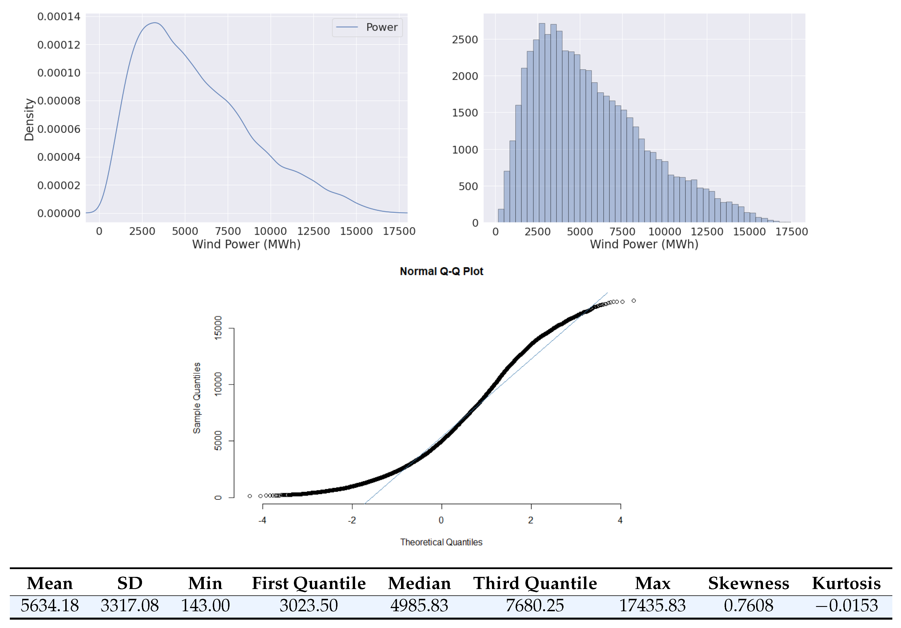
2.1. Dataset Description

Unlike most of the papers available in the literature that deal with the prediction in a turbine or a group of turbines, in this paper, the performance of a suite of LSTM RNN-based models is evaluated on a whole system wind power forecasting. In other words, the historical data in our study case not only depend on wind resource availability in all power system farms but also the balance between offer and supply in the particular electricity market. In this way, remarkable particularities make the Spanish study case attractive to evaluate the performance of forecasting techniques. First, Spain is the fifth country in the world in terms of installed wind power, after China, the US, Germany, and India. There are currently 1265 wind farms installed in 16 out of the 17 states (autonomous communities), covering 21.9% of the energy consumed in the country, making the participation of wind power in the Spanish electricity market substantial [36]. Second, the time series of Spain exhibits a high level of seasonality and trend because of the intrinsic nature of wind resources in the region. Finally, because of the interconnections with Portugal and France, the dataset reflects the behavior of other markets with different energy mixes and the state of the cross-border interconnections. These characteristics make this a challenging study case to evaluate the suitability of the LSTM RNN-based models in forecasting.
In this context, the original dataset for this study covers approximately six and a half years of hourly wind power observations in Spain, collected from the Spanish Electric Network [37]. Specifically, the wind power time series was recorded from 1 January 2014 to 30 May 2020 and reported in megawatts-hour (MWh) for a total of 56,231 observations. Figure 1 represents the wind power data processed and analyzed in this work. Firstly, in order to remove innovational outliers, additive outliers, or level shifts, the approach described in [38] was used for the automatic detection and removal of outliers in the time series. This strategy uses spatial outlier detection by implementing the variogram method, where outliers are considered those that considerably deviate from the majority of the data. This methodology assumes that the outliers are not correlated in time and space, and can be modeled using an α -stable distribution. The selection of this approach was based on its extensive use in the time series preprocessing [39]. Taking this approach into account, no outlier was found in the analysis of the whole time series. Initial observations on the data suggest that there are no changes in trend over the years. In addition, there are relevant peaks at the beginning of each year, marking the annual seasonality of the wind power time series. These ideas are explored in more detail below.
In order to describe the wind power time series analyzed in this work, in Figure 2, the sample descriptive statistics, its corresponding histogram distribution, and the Quantile–Quantile (QQ) plot are summarized. Based on the reported results, it can be seen that the skewness value describes a non-normal wind power time series with a right-skewed distribution. Moreover, the calculated Kurtosis value, being less than three, indicates the data are light-tailed and flatter than a normal distribution (platykurtic).

2.2. Deep Learning Strategies for Time Series Forecasting Using LSTM

Deep learning (DL) is a subset of machine learning (ML) that uses restructured multi-layered ANNs to deliver improved accuracy in diverse tasks, such as object detection, speech recognition, language translation, among many other applications. Given the success of DL models in tackling classification and regression problems, research continues to move towards implementing diverse DL model architectures for a plethora of applications. A particular DL model architecture has gained popularity over the years given its success in handling long and short-term time dependencies and its ability to work with raw time series data without extensive feature engineering or data preprocessing. This DL model is known as RNNs.

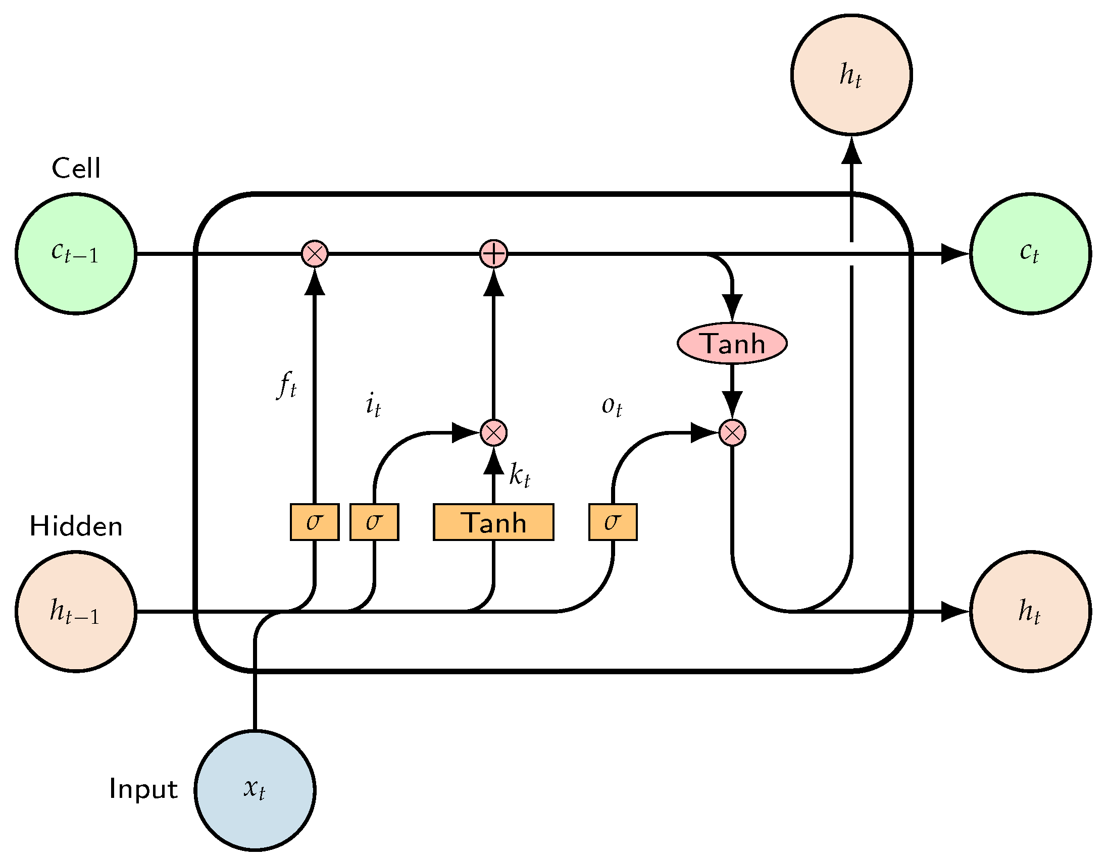
2.2.1. LSTM RNNs Based Models Description

RNNs are dynamic systems that efficiently use the temporal information of a model’s input sequences. For this reason, they are a widely used tool for time series forecasting. RNNs are derived from feed-forward neural networks (FFNN), where the network is forward propagated according to the number of time steps per sample. RNNs are composed by a memory gate that allows the network to process sequential data, maintaining previous inputs to predict the outputs. The RNN model updates its memory, also known as its recurrent hidden state h t , as follows:
h t = σ W x x t + W h h t 1 + b t
where x = ( x 1 , x 2 , , x t ) is a sequence of length t, σ is a nonlinear function such as sigmoid or rectified linear unit (ReLu), W x and W h are weight matrices, and b t is a constant bias value [40]. Standard RNNs suffer from short-term memory and are limited to look back in time, such that the larger the size of the input learning sequence, the less it learns. Moreover, RNNs struggle with long sequential data, leading to exploding and vanishing gradients, where the former refers to the assignment of high importance to the weight matrices without any reason and the latter refers to significantly small gradient values that prevent the RNN model from learning further [40].
LSTM networks address the short-term memory problem of RNNs that leads to vanishing and exploding backpropagation error signals that either grow or shrink with every time step in RNNs. In order to overcome this problem, gated units to control the information flow have been proposed. Specifically, LSTM units have reported successful results in different fields to forecast time series [8,11]. LSTM networks are capable of modeling long-term dependencies in time series, learning more than 1000-time steps, whereas RNNs are limited to 10 steps [41]. Given the competency of LSTM networks in handling long and short-term time dependencies, the study developed in this work utilizes a suite of LSTM-based models to better capture the real-time dynamics of wind energy.

2.2.2. Vanilla LSTM

The traditional LSTM network structure is composed of three gates: the forget gate, the input gate, and the output gate. The forget gate determines which information is valuable enough to be maintained within the network, assigning a value between 0 and 1. Values close to 0 are discarded, while values close to 1 are kept. The input gate decides what information is allowed to flow into the memory cell and be stored there.
Equations (3) and (4) below represent this decision, where k t produces a vector of new values to be added to the memory cell based on the update signal given by i t . The network is then updated as defined in Equation (5), where c t (long-term state) considers whether to keep or forget the previous values and add new values. Lastly, the output of h t (short-term state) is also composed by two layers. Here, o t is the output value given by the σ activation, which determines what values from the memory cell are to be considered as output, followed by a tanh layer with an output range [−1, 1] [42]. Equations (2)–(7) show how the network is updated, which was also illustrated in Figure 3.
f t = σ W f . [ h t 1 , x t ] + b f
i t = σ W i . [ h t 1 , x t ] + b i
k t = tanh W k . [ h t 1 , x t ] + b k
c t = f t × c t 1 + i t × k t
o t = σ W o . [ h t 1 , x t ] + b o
h t = o t × tanh ( c t )
where f t , i t , k t , o t are the output values of the forget gate, input gate, update signal, and output gate, respectively, and their input values are x t at the current time t and the output value h t 1 at time t 1 . W f , i , k , o are weight matrices and b f , i , k , o are bias vectors corresponding to the respective gates. σ is a nonlinear activation function and c t is the memory unit.

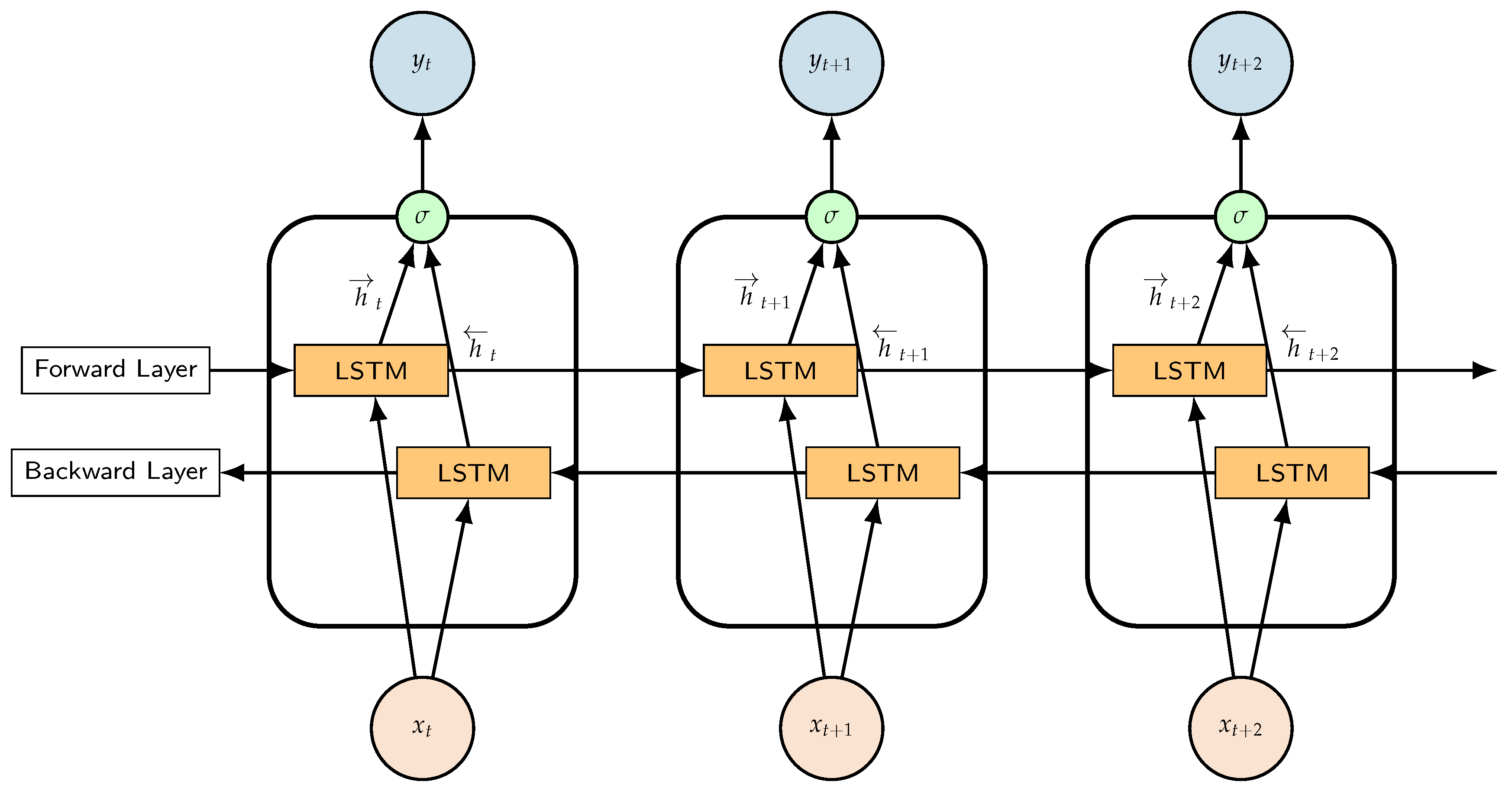
2.2.3. Bidirectional LSTM
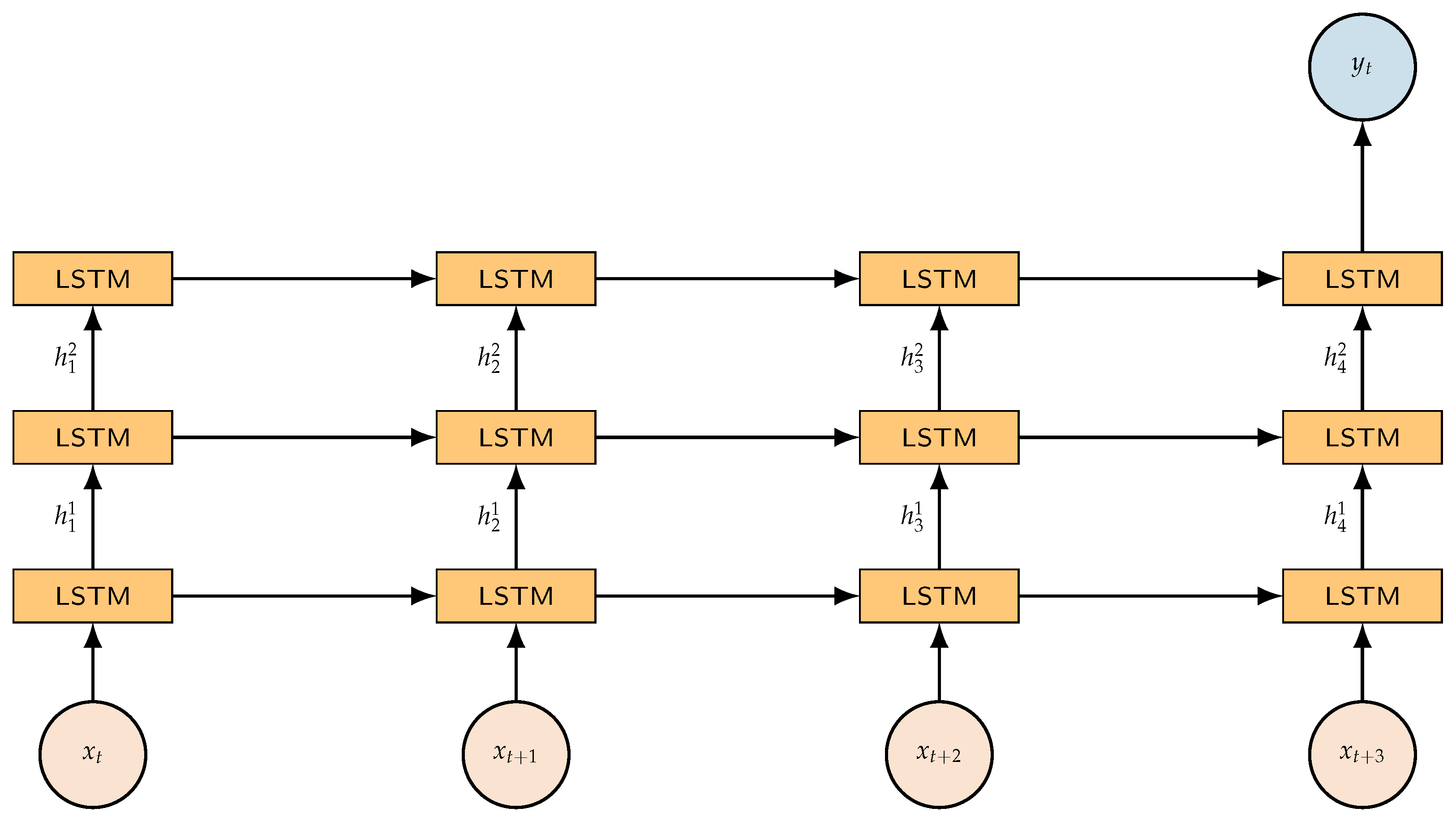
While the vanilla LSTM takes unidirectional processing of the information from left to right, the bidirectional model learns the input time series sequences both forward and backward, ultimately combining both interpretations. The data are processed through independent networks, where one network will process the time series data from left to right, while the other network will process the data from right to left. In this way, each network holds information at time t, while also holding information from either the past or the future. In this case, the hidden state equation is redefined to incorporate the forward layers, backward layers, and combined output. The forward layer’s output sequence h is computed by going through the input sequence from left to right ( t 1 to t n ). In contrast, the backward layer’s output is computed from right to left using the reverse inputs. Ultimately, both outputs are computed as previously defined in Equations (2)–(7).
Figure 4 exemplifies the incorporation of the direction for the forward and backward layers. The concatenated output is defined in Equation (8), where W h y and W h y are the weights of the forward and backward networks, respectively, and b y is the bias of the output layer. Equation (8) can be generalized for multi-step forecasting problems such that y t would be otherwise computed given by y t + 1 , y t + 2 , and so on.
y t = W h y h t + W h y h t + b y

2.2.4. Stacked LSTM

A stacked LSTM refers to a model architecture composed of multiple LSTM layers, making the model deeper. Under a standard LSTM model, the layer would receive an input sequence and output a value or a specified number of values to be predicted. However, under a stacked model, as it is shown in Figure 5, the output of a hidden LSTM layer is not only propagated forward through time but also used as one of the inputs for the next LSTM hidden layer. In this way, the hidden states are a function of all previous hidden states. Consequently, the l-th layer can be updated by the Equations (9)–(14).
f t l = σ W f l . [ h t 1 l , h t l 1 ] + b f l
i t l = σ W i l . [ h t 1 l , h t l 1 ] + b i l
k t l = tanh W k l . [ h t 1 l , h t l 1 ] + b k l
c t l = f t l × c t 1 l + i t l × k t l
o t l = σ W o l . [ h t 1 l , h t l 1 ] + b o l
h t l = o t l × tanh ( c t l )
Based on this configuration, the input associated to the first layer is the raw time series:
h t 0 = x t ,
while its respective output is an input abstraction, which is then fed as a hierarchical feature to the next LSTM layer. The final layer is composed by the number of neurons corresponding to the number of time steps predicted through the model. Different advantages reported for this methodology include that a stacked configuration allows the neural network to learn features from the raw time series in different components at each time step [43]. The parameters associated with the neural network are spread across the whole model’s space, which accelerates the algorithm’s convergence and fine-tunes the nonlinear operations applied to the time series.

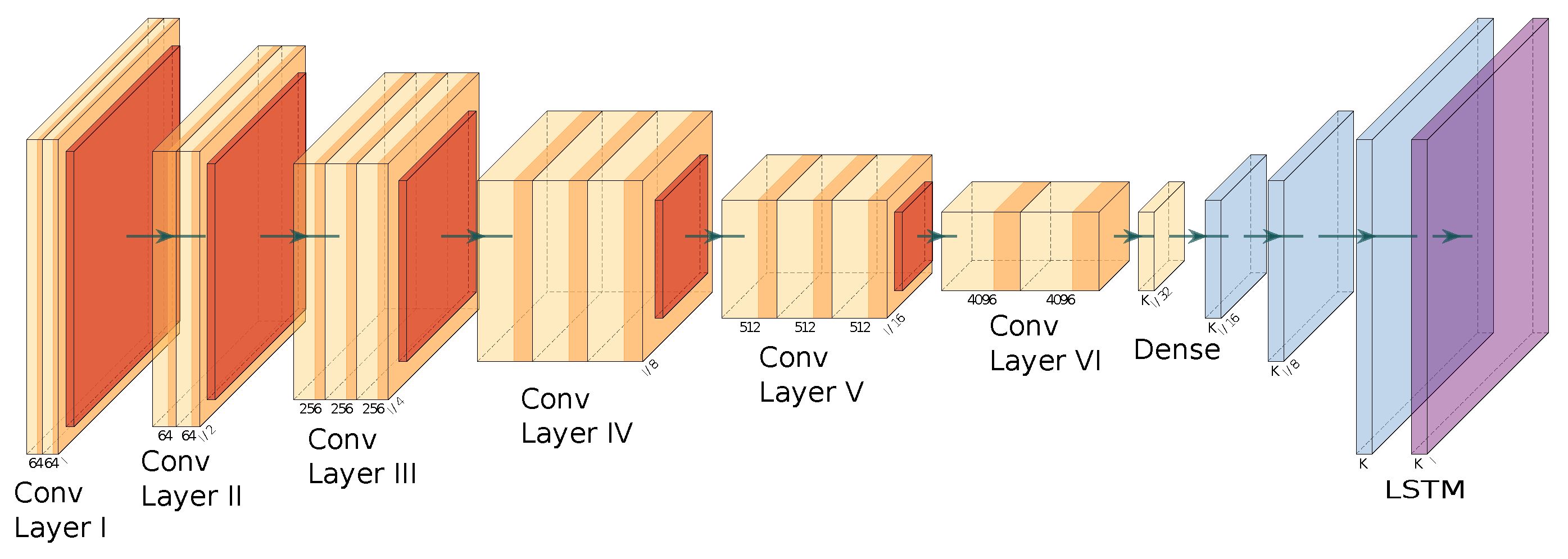
2.2.5. Convolutional LSTM

Convolutional neural networks (CNNs) have been widely used for data feature extraction with grid-like configurations, such as images. The CNN architecture was initially developed for two-dimensional data, allowing the model to learn patterns hierarchically such that the patterns learned will be recognized throughout the network. Presently, one-dimensional CNNs have become more popular given their application to sequence data, such as text and time series. However, their performance is suboptimal when compared to other models, such as LSTMs [44]. CNNs are usually composed by three stacked layers: convolutional layer, pooling layer, and fully connected layer. First, the input layer holds the input vector of values, followed by the convolutional layer where features are extracted through a filter or kernel, to be output into a fully connected layer [45]. The basic structure of CNNs is portrayed in Figure 6. A LSTM network can be connected to the dense or fully connected layer of the CNN configuration as portrayed, such that the convolutional LSTM network would be updated in a similar way as in the vanilla LSTM, replacing the matrix addition and dot product operators by convolutional operators.
A convolutional LSTM RNN (ConvLSTM) incorporates the convolutional structures of the CNN in both the input-to-state and state-to-state transitions. The network is redefined such that the operators previously defined in (2)–(7) are replaced by the convolution operator (∗) and the Hadamard product ( ) as exemplified in Equations (16)–(20), where the latter operator keeps the constant bias property of the cells. As it can be noted, these equations differ from the standard LSTM network in that, in order to extend the LSTM network’s capability to remember or forget information throughout the convolutional LSTM configuration, the information from the cell state is included in all output computations for each gate to take into account the analogous transitions between the states. Moreover, the weight matrices of the respective gates now include a convolution operator in order to incorporate the function of the filter. The network is updated as follows:
i t = σ ( W x i x t + W h i h t 1 + W c i c t 1 + b i )
f t = σ ( W x f x t + W h f h t 1 + W c f c t 1 + b f )
c t = f t c t 1 + i t tanh ( W x c x t + W h c h t 1 + b c )
o t = σ ( W x o x t + W h o h t 1 + W c o c t + b o )
h t = o t tanh ( c t )

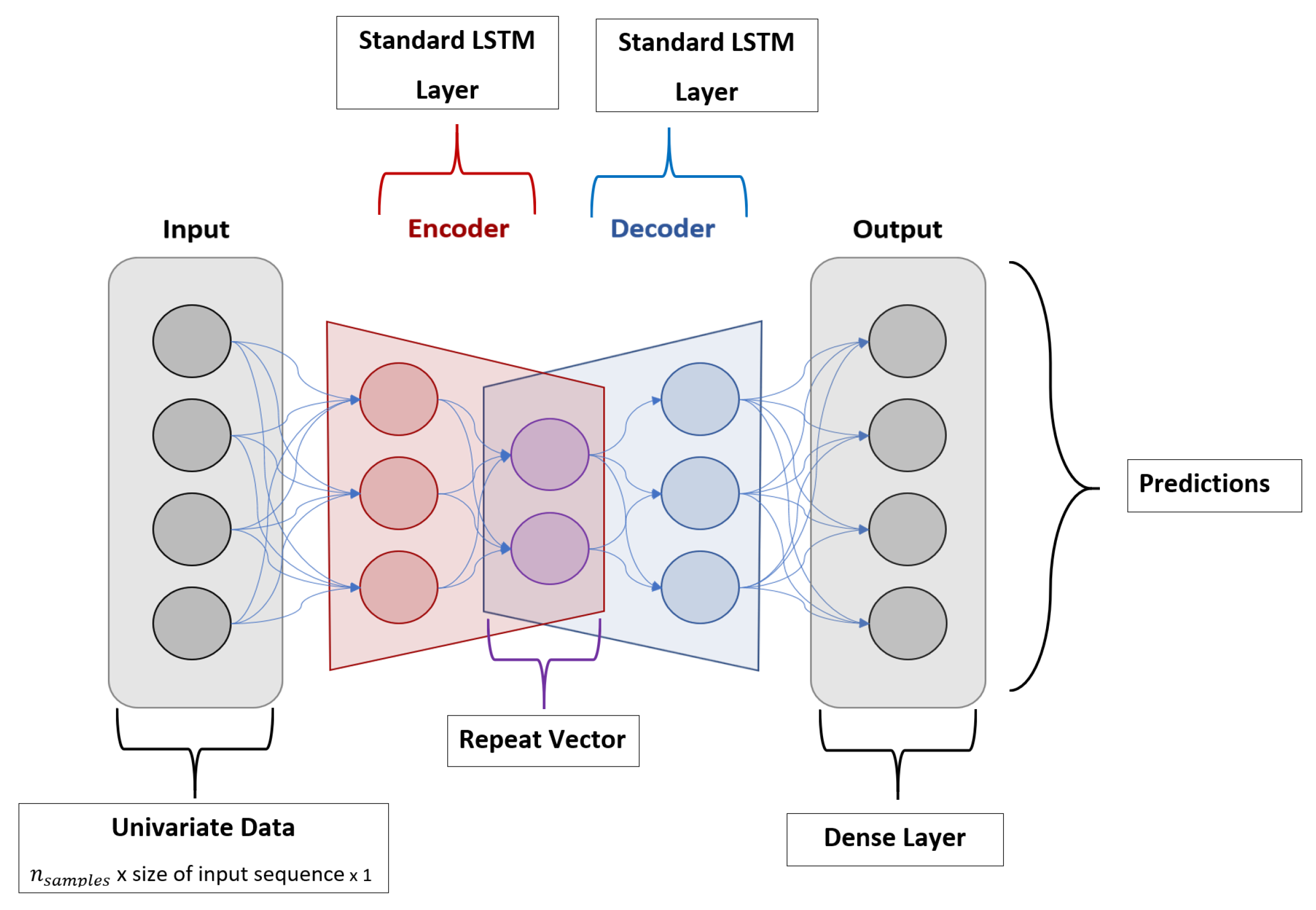
2.2.6. Autoencoder LSTM

The autoencoder (AE) architecture consists of three sequentially connected layers defined as the encoder, the code, and the decoder. AEs extract features from input data in an unsupervised manner and are often used as generative models [44]. The AE architecture is illustrated in Figure 7.
The encoder maps high-dimensional input data into a low-dimensional representation, where the decoder is then responsible for reconstructing the data. This architecture allows the decoder weights to be tuned first, although both the encoder and decoder are trained simultaneously where, ultimately, the model minimizes the difference between the reconstructed output and the original input data. The encoded features e t are given by:
e i = σ ( W e x t + b e )
The decoded values given by the original input data x are given by:
x i ^ = σ ( W d x t + b d )
where σ is the selected activation function, W e is the encoder weight matrix, b e is the encoder bias vector, W d is the decoder weight matrix, and b d is the decoder bias [46]. According to the architecture of AE models, LSTM units can be included in order to process time series, where multiple sequences are taken as input and later as output. This model presents special characteristics to deal with multi-step ahead forecasting, where the output predictions mapped represent several hours to be forecasted at a time.

2.3. Implementation Methodology

Upon completion of the exploratory data analysis, all observations were scaled [0 to 1] for the sake of the networks’ speed, learning rate, and convergence. A data split of 70:30 for training and testing sets is implemented, such that we are able to evaluate the models’ predictive performance for up to two years (at least two periods of annual seasonality). Each model was implemented considering the mathematical background explained in Section 2.2, following the pseudocode presented in Algorithms 1–5. For the LSTM models to learn the mapping function of our historical wind power observations sequence, the original sequence must be transformed into multiple time-series samples from which the LSTM learns. The network maps these sequences as input to an output observation (one-step ahead) or to multiple output observations (multi-steps ahead). Input learning sequence size is based on the weekly seasonal behavior of wind power time series [47]. Considering these characteristics, weekly, monthly, and quarterly time scales have been considered in the preparation of the input data. First, we consider a transformation where 168-time steps are used as input, such that the network learns by week. Then, 720-time steps are proposed, such that the model’s input sequence is equivalent to roughly a month worth of observations. Lastly, we consider a quarterly transformation with 2160-time steps used as input. It must be noted that a larger input sequence size of 8760 steps (annual steps) is not considered due to implications that the size of the time window has on the availability of data for the validation of the models, as we would only have very limited observations as part of the testing dataset. Moreover, the annual input sequence would also require an increasing number of neurons in the hidden layers, which would positively affect the computational times of the networks, which makes the implementation in a timely manner unfeasible.
Algorithm 1 Vanilla LSTM
1:
x RESHAPE(x, shape(168, 720, 2160))
2:
y RESHAPE(y, shape(168, 720, 2160), (1,2,3))
3:
Neurons ← (32,64,128)
4:
Batch Size ← (12, 24, 46, 48)
5:
Epochs ← (100, 200, 300)
6:
Input Learning Sequence ← (168, 720, 2160)
7:
lstm (x, y, Neurons, Batch Size, Epochs, optimizer, loss)
8:
for e ← Input Learning Sequence do
9:
   TRAIN_DATA, VALID_DATA ← TEST_TRAIN_SPLIT(e,0.7)
10:
   for i, j, k ← EPOCHS, Batch Size, Neurons do
11:
     for data ← TRAIN_DATA do
12:
         X data[0], Y data[1]
13:
        prediction_results ← lstm(x,y, i,j,k)
14:
        cost← CALCULATE_COST(prediction_results, y)
15:
        optimizer← ADAM_OPTIMIZER(learning_rate = 0.001).MIN(MSE)
16:
     end for
17:
   end for
18:
end for
Algorithm 2 Stacked LSTM
1:
x RESHAPE(x, shape(168, 720, 2160))
2:
y RESHAPE(y, shape(168, 720, 2160), (1,2,3))
3:
Neurons Layer 1 ← (32,64,128)
4:
Neurons Layer 2 ← (32,64,128)
5:
Batch Size ← (12, 24, 46, 48)
6:
Epochs ← (100, 200, 300)
7:
Input Learning Sequence ← (168, 720, 2160)
8:
lstm (x, y, Neurons Layer 1, Batch Size, Epochs, optimizer, loss)
9:
ADD(lstm, Neurons Layer 2)
10:
Epochs ← (100, 200, 300)
11:
for e ← Input Learning Sequence do
12:
   TRAIN_DATA, VALID_DATA ← TEST_TRAIN_SPLIT(e,0.7)
13:
   for i, j, k, h ← EPOCHS, Batch Size, Neurons Layer 1, Neurons Layer 2 do
14:
     for data ← TRAIN_DATA do
15:
         X data[0], Y data[1]
16:
        prediction_results ← lstm(x, y, i, j, k, h)
17:
        cost← CALCULATE_COST(prediction_results, y)
18:
        optimizer← ADAM_OPTIMIZER(learning_rate = 0.001).MIN(MSE)
19:
     end for
20:
   end for
21:
end for
Algorithm 3 Bidirectional LSTM
1:
x RESHAPE(x, shape(168, 720, 2160))
2:
y RESHAPE(y, shape(168, 720, 2160), (1,2,3))
3:
Neurons ← (32,64,128)
4:
Batch Size ← (12, 24, 46, 48)
5:
Epochs ← (100, 200, 300)
6:
Input Learning Sequence ← (168, 720, 2160)
7:
bilstm (x, y, Neurons, Batch Size, Epochs, optimizer, loss)
8:
for e ← Input Learning Sequence do
9:
   TRAIN_DATA, VALID_DATA ← TEST_TRAIN_SPLIT(e,0.7)
10:
   for i, j, k ← EPOCHS, Batch Size, Neurons do
11:
     for data ← TRAIN_DATA do
12:
         X data[0], Y data[1]
13:
        prediction_results ← bilstm(x, y, i, j, k)
14:
        cost← CALCULATE_COST(prediction_results, y)
15:
        optimizer← ADAM_OPTIMIZER(learning_rate = 0.001).MIN(MSE)
16:
     end for
17:
   end for
18:
end for
Algorithm 4 CNN LSTM
1:
x RESHAPE(x, shape(168, 720, 2160)
2:
y RESHAPE(x, shape(168, 720, 2160), (1,2,3))
3:
Neurons ← (32,64,128)
4:
Batch Size ← (12, 24, 46, 48)
5:
Epochs ← (100, 200, 300)
6:
Input Learning Sequence ← (168, 720, 2160)
7:
Filter ← 24
8:
Kernel Size ← 1
9:
Pool Size ← 2
10:
conv ←RELU_ACTIVATION_FUNC(CONV1D(x, y, Filters, Kernel Size ))
11:
conv ← ADD(conv,MAX_POOL1D(conv, Pool Size)
12:
conv.lstm ← ADD(conv, lstm)
13:
conv.lstm← RESHAPE(conv.lstm)
14:
for e ← Input Learning Sequence do
15:
   TRAIN_DATA, VALID_DATA ← TEST_TRAIN_SPLIT(e,0.7)
16:
   for i, j, k ← EPOCHS, Batch Size, Neurons do
17:
     for data ← TRAIN_DATA do
18:
         X data[0], Y data[1]
19:
        prediction_results ← conv.lstm(x, y, i, j, k)
20:
        cost← CALCULATE_COST(prediction_results, y)
21:
        optimizer← ADAM_OPTIMIZER(learning_rate =0.001 ).MIN(cost)
22:
     end for
23:
   end for
24:
end for
Algorithm 5 Autoencoder LSTM
1:
x RESHAPE(x, shape(168, 720, 2160)
2:
y RESHAPE(x, shape(168, 720, 2160), (3))
3:
Neurons ← (32,64,128)
4:
Batch Size ← (12, 24, 46, 48)
5:
Epochs ← (100, 200, 300)
6:
Input Learning Sequence ← (168, 720, 2160)
7:
aulstm(x, y, Neurons, Batch Size, Epochs, Optimizer, Loss)
8:
aulstm← ADD(aulstm, RepeatVector(3))
9:
aulstm← ADD(aulstm, Neurons)
10:
for e ← Input Learning Sequence do
11:
   TRAIN_DATA, VALID_DATA ← TEST_TRAIN_SPLIT(e,0.7)
12:
   for i, j, k ← EPOCHS, Batch Size, Neurons do
13:
     for data ← TRAIN_DATA do
14:
         X data[0], Y data[1]
15:
        prediction_results ← aulstm(x, y, i, j, k)
16:
        cost← CALCULATE_COST(prediction_results, y)
17:
        optimizer← ADAM_OPTIMIZER(learning_rate =0.001 ).MIN(cost)
18:
     end for
19:
   end for
20:
end for
The models are first evaluated, given the different input learning sequences for one-step ahead forecasting. An iterative training process is first implemented to find the DL-based model and configuration with the best performance. Then, the models and their respective configurations, yielding the lowest possible error rate, are selected to evaluate their performance when facing three-steps ahead forecasting. The iterative process is only completed for one-step ahead forecasting due to the exhaustive computational load that the forecasting of three steps entails, considering the different DL architectures. Lastly, we are able to conduct a comparative analysis to evaluate the performance of the three-steps ahead forecasting models against an AE-LSTM model, which is commonly used to tackle multi-step forecasts rather than one step. The general implementation process is shown in Figure 8.
Since batch size relates to the number of training samples to be considered at a time for updating the network, batch size may affect the network speed, learning rate, and convergence. Therefore, different batch sizes are considered according to the number of samples obtained through the selected time windows, such that the samples are divisible by the proposed batch sizes. As such, models set up according to weekly and monthly learning sequences are implemented with batch sizes 12, 24, and 46. In contrast, models set up through a quarterly learning sequence are implemented with batch sizes 12, 24, and 48. Likewise, we select a different number of memory units for the LSTM layers. Since the initial model configurations are based on increasing learning sequence sizes, an increasing number of units is proposed to understand whether more complex models are able to better solve the problem at hand. The number of neurons in each hidden layer play a key role in the neural network training and impact the prediction accuracy [23]. The more the number of neurons in each layer, the more complex the model. Lastly, a varying number of training cycles is proposed (100–300 epochs). In this way, the iterative process will be performed such that the models’ training cycles and batch sizes vary, so the networks are trained with different patterns. Given all the possible hyperparameter configurations portrayed in Table 1, and according to the number of steps in the input sequence, there are 27 possible combinations for each, at minimum, given the number of epochs, size of the batches, and the number of neurons.
The activation function employed is ReLu, as its gradient does not tend to suffer from gradient vanishing or diffusion [46]. In addition, models are trained using the Adam optimization algorithm [48], where the default recommended parameters are used (learning rate = 0.001, β 1 = 0.9, β 2 = 0.999, ϵ = 1 × 10 8 ), unless otherwise stated and required by the model. The Adam optimizer is useful in handling sparse and noisy problems as it combines the properties of AdaGrad and RMSProp optimizers, and is applicable to LSTM time series forecasting as it does not require a stationary objective [48,49]. Additionally, the selection of this model is based on the reported advantages of its implementation to support DL-based models: straightforward implementation without the need of extensive data preprocessing and decomposition methods, small memory requirement, invariance to the diagonal re-scalation of gradients, suitability for models that involve large datasets, and/or large number of parameters [48,49]. Finally, the mean square error (MSE) is the selected loss function to be minimized, based on the successful results reported of this loss function in conjunction with the Adam optimizer [49,50,51].

2.4. Evaluation Metrics

The performance evaluation of the different LSTM models is performed by comparing the root mean square error (RMSE), the mean absolute percentage error (MAPE), the mean absolute error (MAE), and the coefficient of determination (R), defined as:
R M S E = 1 N i = 1 N ( x i x i ^ ) 2
M A P E = 1 N i = 1 N x i x i ^ x i × 100 %
M A E = 1 N i = 1 N | x i x i ^ |
R 2 = 1 i = 1 N ( x i x i ^ ) 2 i = 1 N ( x i x i ¯ ) 2
where N is the number of predicted samples, x i and x i ^ are the real and predicted values, respectively, and x i ¯ is the real values’ mean. RMSE provides the overall agreement between estimated and original data, avoiding error compensation, while the performance in actual units is achieved through root implementation [34]. RMSE has been considered one of the most commonly used indicators for power forecasting in renewable energy stations because it can be used effectively with the satisfaction of objectivity and symmetry criterion. In addition, it can be used uniformly for different measurement durations [52]. In contrast to RMSE, the MAE metric weights all values equally, and thus does not add additional weight to extreme forecasting events. This metric has been widely used in the renewable energy industry to assess the effectiveness of the forecast [53]. MAPE, on the other hand, represents the quantum of error relative to the actual data expressed as percentage, thereby directly indicating the accuracy of the model [54]. This metric has been proposed as the most widely used unit-free accuracy measure for forecasting tasks and it has been recommended by many textbooks, M-competition, and the previous literature [55,56]. Finally, the accuracy is measured using the coefficient of determination R 2 . This metric compares the sum of the square of the residuals with the total sum of squares, which is proportional to the variance of the data. These evaluation metrics have been selected because they are the most used performance measures in the field of short-term wind power forecasting using deep learning techniques [4,5,8,23].

3. Wind Power Forecasting—Experimental Results

Based on the methodology described in the previous section, the experiments for each model were carried out. It is important to note that every model was compiled in Python 3.8 with Tensor Flow 2.4.0 backend and Intel(R) Core(TM) i7-8565U.

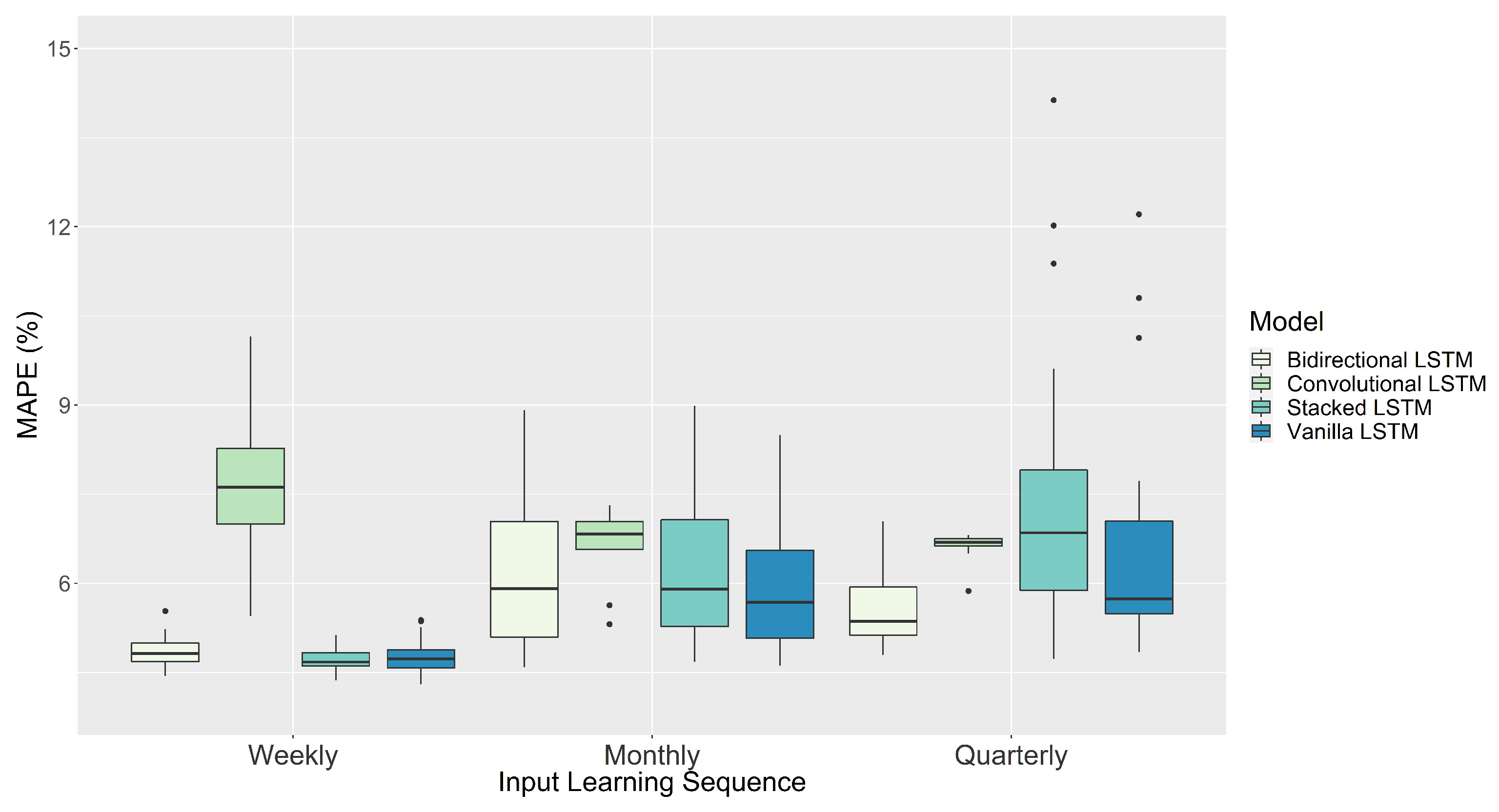
3.1. One-Step Forecasting

First, single-step ahead forecasting strategies were assessed. Single, bi-directional, stacked, and convolutional LSTM RNNs were implemented according to the previously defined implementation process, varying the number of input neurons with only one output defined by the value to be predicted.
Given the hyperparameter configurations portrayed in Table 1, and according to the number of steps in the input sequence, there are 27 possible combinations for each given the number of epochs, size of the batches, and the number of neurons in the hidden layer. The first technique implemented was the vanilla LSTM. The performance of each model is illustrated in Figures S1–S3 of the Supplementary Material. For this approach, the smallest MAPE error of 4.30% was recorded under a configuration of 168-time steps corresponding to a weekly input learning, 200 iterations, batch size of 46, and 32 neurons in the hidden layer. The models implemented using monthly input sequences produced errors between 4.61 and 8.49%, while the quarterly input sequence models reported errors between 4.84 and 12.21%. It is possible to see that, as the size of the input learning sequences increase, so do their corresponding error metrics.
The bidirectional LSTM models were implemented using all possible configuration parameters referenced in Table 1. Once again, as it can be seen in Figures S4–S6 of the Supplementary Material, the best performing model configuration, with a reported MAPE of 4.44%, is given by the model that learned by weekly time steps (168 steps) implemented with 200 epochs, batch size of 46, and 32 neurons. However, the highest reported error rates were found within the implementation with monthly time steps (720 steps), where the errors ranged between 4.60 and 8.91%. In comparison, the models implemented with quarterly time steps (2160 steps) produced a 4.79–7.04% range. Overall, the models initiated with weekly time steps maintained values between 4.44 and 5.53%, resulting in lower variability among the reported metrics. This architecture maintained similar metrics for the weekly and monthly input sequence implementations, and it improved the resulting error range under the quarterly input steps. In contrast, the range for the vanilla for the quarterly input sequence (2160 steps) was 4.84–12.21%, the bidirectional reported a range of 4.79–7.04%, resulting in lower variability.
In addition, a stacking architecture with two LSTM layers is implemented, where each layer is independent, and the number of neurons in each layer may vary between 32 or 64 neurons, being these two values the most commonly employed under stacked architectures [57,58]. Under this configuration, we exclude the implementation of 128 neurons for the sake of implementation times as a higher number of neurons may prevent the models from finding a solution within a suitable time frame. A dense layer then connects the layers with one neuron for a single time step output. Given all the possible parameter configurations portrayed in Table 2, there are a total of 108 possible combinations given the size of the input sequence, iterations, size of the batches, and the number of neurons in the first and second layers.
Figures S7–S9 of the Supplementary Material show the MAPE reported for stacked LSTM models with 32 neurons on the first layer and a varying number of neurons on the second layer. The lowest recorded error of 4.37% was produced by the model implemented with 32 memory units in the first and second layers, 300 epochs, a batch size of 12, and a weekly input sequence (168 steps). The models implemented under the monthly input sequence yielded errors ranging from 4.68 to 8.82%, while the quarterly sequence approach produced errors ranging between 4.75 and 9.37%. The results for the stacked model with 64 neurons on the first layer are portrayed below in Figures S10–S12 of the Supplementary Material. Once again, the lowest recorded MAPE of 4.50% was produced by the model configured with an input sequence of size 168, 32 neurons in the second layer, 300 epochs, and batch size of 12. The models implemented under the monthly input sequence yielded MAPE errors ranging from 4.70 to 8.99%, while the quarterly sequence approach yielded errors ranging between 4.73 and 14.13%. Overall, the models implemented with a weekly input sequence (168 steps) produced the lowest MAPEs ranging between 4.37 and 5.13%. The lowest reported error (4.37%) was produced by the model configured with 32 neurons on the first and second layers, 300 epochs, and a batch size of 12. This architecture achieves a slightly lower variability in relation to weekly input sequence (168 steps) implementations when compared to the vanilla (4.30–5.38%) and bidirectional (4.44–5.53%) models.
The Conv-LSTM implementation, on the other hand, considers some fixed parameters based on the results reported previously in the literature. As such, for these experiments, 64 filters were used in the convolutional layer and a max-pooling kernel size of 2. This parameter configuration has been previously employed in studies of short-term wind power forecasting [42]. This model required a further split of the input sequences into subsequences to take advantage of the feature extraction capability. Given the already established data splits (168, 720, 2160 input sequence), each sample is split into smaller samples. Our selection splits every sample by 24 h for the model to read subsequences equivalent to daily data. In this way, the number of subsequences per sample, according to input sequences of sizes 168 (weekly), 720 (monthly), and 2160 (quarterly), is 7, 30, and 90, respectively. Given the additional subsequences, only the models initialized with weekly input time steps (168 steps) were processed considering all the other possible configurations of the hyperparameters referenced in Table 1. This was due to the significant increase in computational times of this architecture that made their implementation infeasible. The results, using the full suite of possible configurations given a weekly input learning sequence (168 steps), were produced in roughly 22 h (Figure S13 of the Supplementary Material). However, the results given monthly and quarterly input time steps, implemented with 100 epochs only, took 27 and 57 h, respectively (Figures S14 and S15 of the Supplementary Material). Under these Conv-LSTM configurations, the MAPE results range from 5.45 to 10.15, 5.31 to 7.31, and 5.87 to 6.81%, given weekly (168 steps), monthly (720 steps), and quarterly (2160 steps) input learning sequences, respectively. While the previously analyzed architectures produced the lowest error variability under weekly input sequences, the Conv-LSTM produced the lowest error variability according to the quarterly input sequence implementations (5.87–6.81%). The lowest reported MAPE of 5.31% was found under monthly input time steps (720 steps), 100 epochs, batch size of size 12, and 128 neurons.
For one-step ahead wind power forecasting, according to the overall performance results recorded in Table 3 and portrayed in Figure 9, it can be observed that the majority of the architectures produce better results when implemented with an input learning sequence of 168 steps (weekly time steps). Further, it is possible to observe that the trade-off between the error metric results and implementation times is not valuable enough to choose a more complex nor deeper model (stacked-LSTM or Conv-LSTM). While the standard and bidirectional models yielded MAPEs between 4.30–12.21 and 4.44–8.91%, the stacked and convolutional architectures produced errors between 4.37–14.13 and 5.45–10.15%, respectively. Additionally, standard and bidirectional models were able to implement all proposed hyperparameter configurations, referenced in Table 1, in approximately 23 and 40 h, respectively. In contrast, the stacked and convolutional models involved implementations between 32 and 106 h, respectively. As the size of the input time steps increased, so did the associated error variability and the implementation times. However, the increase in execution times is also positively related to the number of neurons and the complexity of the models.

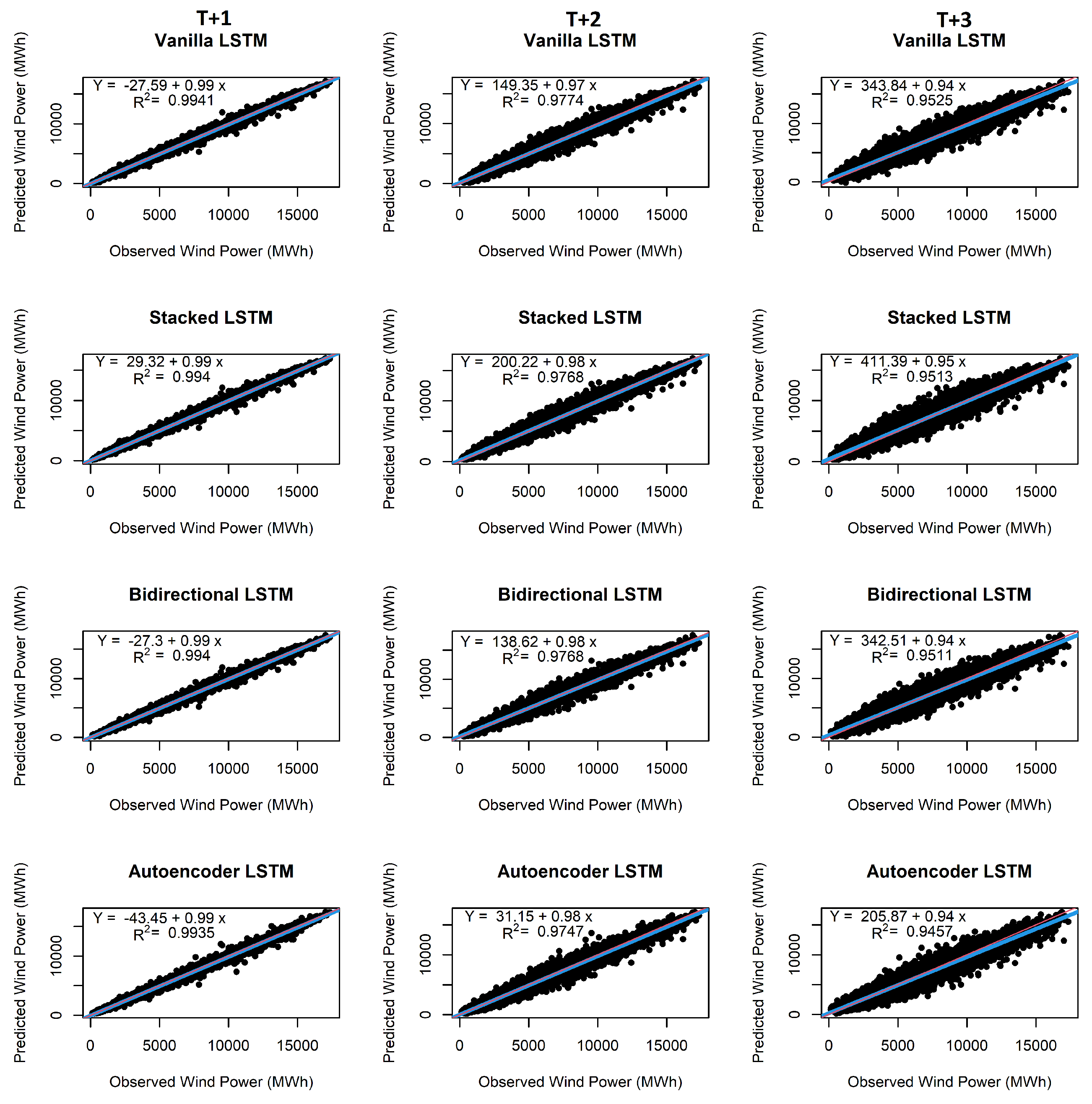
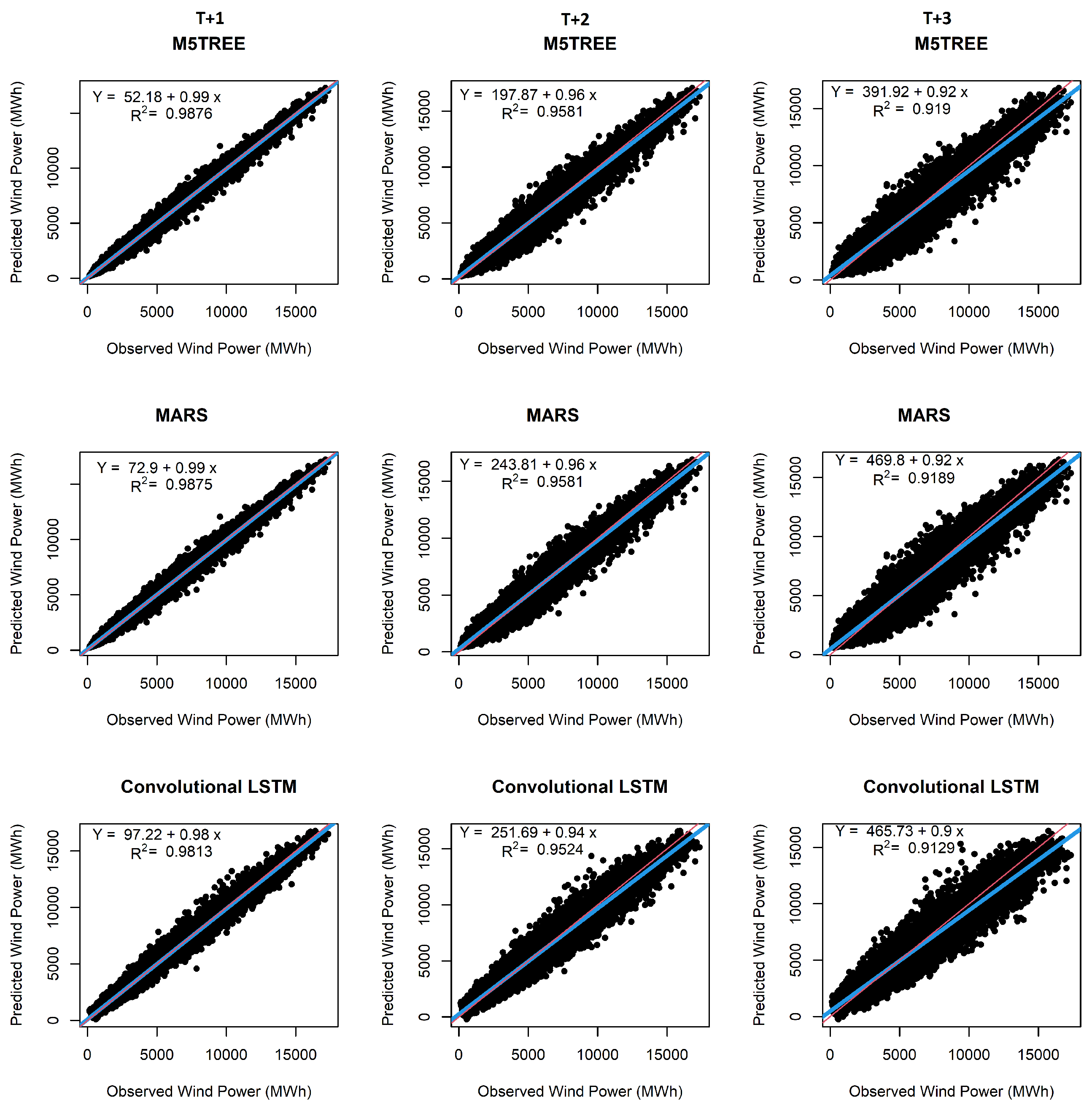
3.2. One-to-Three-Steps Forecasting

Given the results of the one-step forecasting models implemented in the previous section, now, the model configurations that produced the lowest errors are selected to carry out a forecasting three steps ahead. Lastly, an autoencoder LSTM architecture is introduced for this task to compare its performance against the previously studied models. This DL architecture is only presented for the three-steps ahead forecasting task due to its inner configurations, where multiple neurons are found at the input and output layers.
The one-step LSTM model that yielded the best predictive performance had a configuration of weekly input time steps (168 steps), 200 iterations, batch size of 46, and 32 neurons in the hidden layer, with an error rate of 4.30%. Based on this configuration, the model was updated such that there are three neurons in the output layer, instead of 1, to produce the three-steps ahead predictions. The reported MAPE and RMSE increased with each further time step predicted, as has been reported in the literature, ranging from 4.47 to 13.61% and from 269.64 to 745.22 MW, respectively (Figure S16 of the Supplementary Material).
In the same way, the best performing one-step BiLSTM model configuration, with a reported MAPE of 4.44%, was given by a configuration of 168 input time steps implemented with 200 epochs, batch size of 46, and 32 neurons. Based on this configuration, the model was updated such that there are three neurons in the output layer, instead of 1, to produce the three-steps ahead predictions. The three-steps ahead forecast we implemented with this configuration produced almost identical results for the first hour predicted, yet it also proved that the MAPE errors increase with each additional hour forecasted, ranging from 4.50 to 13.27%, which translates into 267.95–741.82 MWh.
Under the lowest error yielding configuration for the stacked LSTM referenced in Table 3, the model was updated such that there are three neurons in the output layer, instead of 1, to produce the three-steps ahead predictions. The stacked architecture has produced a lower MAPE, MAE, and RMSE for the first step predicted in comparison to the vanilla and bidirectional three-steps ahead models; however, these previous implementations showcase a better performance for the second and third hours predicted.
According to the Conv-LSTM results presented in Table 3, the model was updated such that there are three neurons in the output layer, instead of 1, to produce the three-steps ahead predictions. The model’s performance for this task proves to be the highest error-yielding network compared to the previous architectures, as all error metrics for each step have virtually doubled under this configuration, with a MAPE between 8.24 and 17.21% and a RMSE between 463.22 and 962.18 MWh.
Finally, the AE-LSTM networks are introduced given their encoder and decoder architecture, which is especially helpful in multi-step forecasting given their generative capabilities. The recorded metrics for this first implementation show that there is little variation among the models implemented with a different number of neurons in the hidden layer. Overall, the hyperparameter configuration yields the lowest MAPE by the implementations set up with a batch of size 46 and 32 neurons, ranging between 4.24 and 13.03%. At the same time, the reported RMSE for this model produced negligible differences in terms of MWh. For executing the models according to a monthly input sequence (720 steps), 32 and 64 neurons were considered during the parameters tuning process. Lastly, the models with quarterly-sized input sequences (2160 steps) had to be trimmed down due to the extreme computation time that made the implementation unfeasible using more than 32 neurons in the hidden LSTM layer. Results are portrayed in Figure S22 of the Supplementary Material. The lowest reported MAPE ranges between 4.19 and 12.60% and is related to the model with 32 neurons and a batch size of 12.
As a performance summary, the three-steps ahead forecasting executions suffered from high implementation times and computational load, and the overall observed metrics variations did not justify the selection of deeper nor more complex models. Table S1 in the Supplementary Material shows the overall performance of the AE-LSTM model implemented with varying hyperparameters. The implementation times under the AE-LSTM model architecture are extremely high; however, the vast majority of the recorded metrics produced similar results regardless of the input learning sequence size and suffered less variations among the metrics when compared to the reported performance of the other models. Table 4 shows the overall performance of the vanilla, stacked, bidirectional, autoencoder, and convolutional models implemented given the configurations that yielded the lowest error, also including reported metrics for MARS and M5Tree models, as statistical baseline models. In summary, it can be observed in those results that for multi-steps ahead (2–3) the bidirectional LSTM shows the best performance, providing the best trade-off between computation time and lowest recorded MAE, MAPE, and RMSE for the different number of steps ahead considered in this study. These results can be explained considering that bidirectional LSTM-based models can exploit the temporal correlations in the time series data in both forward and backward directions. In addition, taking into account the presented study case, where the time series have a characteristic seasonality, the bidirectional approach provides better feature representation as compared to vanilla and stacked LSTM structures. Regarding to the R 2 results, the vanilla, stacked, bidirectional, and autoencoder LSTM models have similar values, with slightly better performance for the vanilla LSTM.
Figure 10 shows the scatter diagrams of the obtained results for 1-step, 2-steps, and 3-steps ahead predictions. According to the results, it can be seen that the vanilla, stacked, bidirectional, and autoencoder LSTM models present the best performance, while the convolutional LSTM has comparable results to MARS and M5Tree. As expected, the best results were obtained in T + 1 prediction, while T + 2 and T + 3 predictions followed the T + 1, respectively. In general, the results do not reveal significant differences between autoencoders, bidirectional, and LSTM models, according to the determination coefficient. The scatter plots clearly revealed that these last models’ outputs are more aligned to the 1:1 perfect line for T + 1 prediction, while for T + 2 and T + 3, the determination coefficient is smaller.

4. Conclusions

The suite of LSTM RNN-based models presented in this study, along with the diverse patterns in which each architecture was implemented, allowed for a vast comparative analysis for one-step to three-steps ahead wind power forecasting. LSTM models configured in standard, bidirectional, stacked, encoder/decoder, and also coupled with a CNN model, were executed with varying input learning sequences defined as weekly (168 time steps), monthly (720 time steps), and quarterly (2160 time steps). In addition, the diverse model architectures were implemented through an iterative process, where different hyperparameters were varied, such that the models learned in different patterns. This implementation process was executed in order to tackle one-step and three-steps ahead wind power predictions.
For one-step ahead wind power forecasting, the results showed that the majority of the architectures produced better results when implemented with an input learning sequence of 168 steps (weekly time steps). In particular, while the standard and bidirectional models yielded MAPEs between 4.30–12.21 and 4.44–8.91%, the stacked and convolutional architectures produced errors between 4.37–14.13 and 5.45–10.15%, respectively. The three-steps ahead forecasting executions suffered from high implementation times and computational load, and the overall observed metrics variations did not justify the selection of deeper nor more complex models.
The model with the best performance in forecasting one-hour ahead wind power is the stacked LSTM, implemented with weekly learning input sequences, with an average MAPE improvement of roughly 6, 7, and 49%, when compared to standard, bidirectional, and convolutional LSTM models, respectively. In the case of two- or three-hours ahead forecasting, the model with the best overall performance is the bidirectional LSTM implemented with weekly learning input sequences, showcasing improved performance from 2 to 23% when compared to the other LSTM architectures implemented.
While the study completed within this work fills in some of the research gaps concerning DL comparative analysis and hyperparameter optimization, we have laid the blueprint for future research focused on LSTM-RNN architectures for short-term forecasting in the field of wind energy applications. In order to complement the presented comparative analysis, other study cases could be analyzed to determine the performance of these techniques under different wind power and electricity market dynamics, as well as different weight of the wind resources in the energy mix in a power system. Given the increasing implementation times and computational load of the more complex models, future works may consider the incorporation of parallel or high performance computing (HPC) in order to efficiently solve the forecasting tasks at hand, consider more hyperparameters to be included in the iterative process, and assess even deeper models.
As a final conclusion, it is well known that the high variability of wind power makes it difficult to predict their energy output. In fact, the unpredictability of the wind energy could reduce system reliability and increase power curtailments in power systems. Consequently, additional support mechanisms and policies are needed to deal with wind power uncertainty. In this way, accurate wind power forecasting based on DL strategies could boost the security of electricity supply and help guide the policies and decision making in power systems. Precise forecasting helps to design policies estimating suitable reinforcements and reserves needed in the power system according to the wind energy shortages. Furthermore, it could help build realistic scenarios to develop support mechanisms to reduce the firms’ risk exposure in the short-term electricity markets.

Supplementary Materials

Author Contributions

Conceptualization, E.M., G.M. and J.C.; methodology, E.M., G.M. and J.C.; formal analysis, E.M.; investigation, J.C. and G.M.; resources, E.M., J.C. and G.M.; data curation, E.M. and G.M.; writing—original draft preparation, E.M., G.M. and J.C.; writing—review and editing, E.M., G.M. and J.C.; visualization, E.M.; supervision, J.C. and G.M. All authors have read and agreed to the published version of the manuscript.

Funding

This research received no external funding.

Institutional Review Board Statement

Not applicable.

Informed Consent Statement

Not applicable.

Conflicts of Interest

The authors declare no conflict of interest.

Abbreviations

The following abbreviations are used in this manuscript:
AEAutoencoder
ANNArtificial Neural Network
ARIMAAutoregressive Integrated Moving Average Model
BPNNBack Propagation Neural Networks
ConvLSTM    Convolutional LSTM
CNNConvolutional Neural Network
DEDifferential Evolution
DLDeep Learning
DWDiscrete Wavelet Transform
ESNEcho State Network
FFNNFeed-Forward Neural Networks
GAGenetic Algorithm
GHGGreenHouse Gas
GLSTMGenetic Long Short-Term Memory
KFKalman filter
LMBNNLevenberg–Marquardt Backpropagation Neural Network
LSTMLong Short-Term Memory
MAPEMean Absolute Percentage Error
MARSMultivariate Adaptive Regression Splines
MLMachine Learning
MSEMean Square Error
NWPNumerical Weather Prediction
PCAPrincipal Component Analysis
QQQuantile–Quantile
RMSERoot Mean Square Error
RNNRecurrent Neural Network
STSR-LSTMSequence-to-sequence Long Short-term Memory Regression
SVMSupport Vector Machine
VMDVariational Mode Decomposition

References

  1. Tong, W. Wind Power Generation and Wind Turbine Design, 1st ed.; WIT Press: Billerica, MA, USA, 2010. [Google Scholar]
  2. Renewables 2020 Global Status Report. 2020. Available online: https://ren21.net/gsr-2020/ (accessed on 1 August 2021).
  3. Li, L.; Lin, J.; Wu, N.; Xie, S.; Meng, C.; Zheng, Y.; Wang, X.; Zhao, Y. Review and outlook on the international renewable energy development. Energy Built Environ. 2020, in press. [Google Scholar] [CrossRef]
  4. Giebel, G.; Kariniotakis, G.; Brownsword, R. The state-of-the-art in short term prediction of wind power from a danish perspective. In Proceedings of the 4th International Workshop on Large Scale Integration of Wind Power and Transmission Networks for Offshore Wind Farms, Billund, Denmark, 20–21 October 2003. [Google Scholar]
  5. Du, P.; Wang, J.; Yang, W.; Niu, T. A novel hybrid model for short-term wind power forecasting. Appl. Soft Comput. 2019, 80, 93–106. [Google Scholar] [CrossRef]
  6. Marulanda, G.; Bello, A.; Cifuentes Quintero, J.; Reneses, J. Wind Power Long-Term Scenario Generation Considering Spatial-Temporal Dependencies in Coupled Electricity Markets. Energies 2020, 13, 3427. [Google Scholar] [CrossRef]
  7. Ren, Y.; Suganthan, P.; Srikanth, N. Ensemble methods for wind and solar power forecasting—A state-of-the-art review. Renew. Sustain. Energy Rev. 2015, 50, 82–91. [Google Scholar] [CrossRef]
  8. Cao, Y.; Gui, L. Multi-Step wind power forecasting model Using LSTM networks, Similar Time Series and LightGBM. In Proceedings of the 2018 5th International Conference on Systems and Informatics (ICSAI), Nanjing, China, 10–12 November 2018; pp. 192–197. [Google Scholar] [CrossRef]
  9. Abdelaziz, A.Y.; Rahman, M.A.; El-Khayat, M.; Hakim, M. Short term wind power forecasting using autoregressive integrated moving average modeling. In Proceedings of the 15th International Middle East Power Systems Conference, Alexandria, Egypt, 23–25 December 2012. [Google Scholar]
  10. Cifuentes, J.; Marulanda, G.; Bello, A.; Reneses, J. Air temperature forecasting using machine learning techniques: A review. Energies 2020, 13, 4215. [Google Scholar] [CrossRef]
  11. Rodriguez, M.A.; Sotomonte, J.F.; Cifuentes, J.; Bueno-López, M. A Classification Method for Power-Quality Disturbances Using Hilbert–Huang Transform and LSTM Recurrent Neural Networks. J. Electr. Eng. Technol. 2020, 16, 249–266. [Google Scholar] [CrossRef]
  12. Eseye, A.; Zhang, J.; Zheng, D.; Shiferaw, D. Short-Term Wind Power Forecasting Using Artificial Neural Networks for Resource Scheduling in Microgrids. Int. J. Sci. Eng. Appl. 2016, 5, 144–151. [Google Scholar] [CrossRef]
  13. Shi, J.; Liu, Y.; Yang, Y.; Lee, W. Short-term wind power prediction based on wavelet transform-support vector machine and statistic characteristics analysis. In Proceedings of the 2011 IEEE Industrial and Commercial Power Systems Technical Conference, Newport Beach, CA, USA, 1–5 May 2011; pp. 1–7. [Google Scholar] [CrossRef] [Green Version]
  14. Makhloufi, S.; Pillai, G.G. Wind speed and wind power forecasting using wavelet denoising-GMDH neural network. In Proceedings of the 2017 5th International Conference on Electrical Engineering-Boumerdes (ICEE-B), Boumerdes, Algeria, 29–31 October 2017; IEEE: Piscataway, NJ, USA, 2017; pp. 1–5. [Google Scholar]
  15. Elattar, E.E.; Goulermas, J.Y.; Wu, Q.H. Generalized locally weighted GMDH for short term load forecasting. IEEE Trans. Syst. Man Cybern. Part (Appl. Rev.) 2011, 42, 345–356. [Google Scholar] [CrossRef]
  16. Yuan, X.; Chen, C.; Yuan, Y.; Huang, Y.; Tan, Q. Short-term wind power prediction based on LSSVM–GSA model. Energy Convers. Manag. 2015, 101, 393–401. [Google Scholar] [CrossRef]
  17. Tascikaraoglu, A.; Uzunoglu, M. A review of combined approaches for prediction of short-term wind speed and power. Renew. Sustain. Energy Rev. 2014, 34, 243–254. [Google Scholar] [CrossRef]
  18. Yildiz, C.; Acikgoz, H.; Korkmaz, D.; Budak, U. An improved residual-based convolutional neural network for very short-term wind power forecasting. Energy Convers. Manag. 2021, 228, 113731. [Google Scholar] [CrossRef]
  19. Shewalkar, A.; Nyavanandi, D.; Ludwig, S.A. Performance evaluation of deep neural networks applied to speech recognition: RNN, LSTM and GRU. J. Artif. Intell. Soft Comput. Res. 2019, 9, 235–245. [Google Scholar] [CrossRef] [Green Version]
  20. Li, P.; Zhou, K.; Lu, X.; Yang, S. A hybrid deep learning model for short-term PV power forecasting. Appl. Energy 2020, 259, 114216. [Google Scholar] [CrossRef]
  21. Althelaya, K.A.; El-Alfy, E.S.M.; Mohammed, S. Stock market forecast using multivariate analysis with bidirectional and stacked (LSTM, GRU). In Proceedings of the 2018 21st Saudi Computer Society National Computer Conference (NCC), Riyadh, Saudi Arabia, 25–26 April 2018; IEEE: Piscataway, NJ, USA, 2018; pp. 1–7. [Google Scholar]
  22. Qu, X.; Kang, X.; Zhang, C.; Jiang, S.; Ma, X. Short-term prediction of wind power based on deep Long Short-Term Memory. In Proceedings of the 2016 IEEE PES Asia-Pacific Power and Energy Engineering Conference (APPEEC), Xi’an, China, 25–28 October 2016; pp. 1148–1152. [Google Scholar] [CrossRef]
  23. Liu, Y.; Guan, L.; Hou, C.; Han, H.; Liu, Z.; Sun, Y.; Zheng, M. Wind Power Short-Term Prediction Based on LSTM and Discrete Wavelet Transform. Appl. Sci. 2019, 9, 1108. [Google Scholar] [CrossRef] [Green Version]
  24. Sun, Z.; Zhao, M. Short-Term Wind Power Forecasting Based on VMD Decomposition, ConvLSTM Networks and Error Analysis. IEEE Access 2020, 8, 134422–134434. [Google Scholar] [CrossRef]
  25. Ye, R.; Suganthan, P.N.; Srikanth, N.; Sarkar, S. A hybrid ARIMA-DENFIS method for wind speed forecasting. In Proceedings of the 2013 IEEE International Conference on Fuzzy Systems (FUZZ-IEEE), New Orleans, LA, USA, 23–26 June 2019; IEEE: Piscataway, NJ, USA, 2013; pp. 1–6. [Google Scholar]
  26. Lee, S.; Kim, J. Predicting Inflow Rate of the Soyang River Dam Using Deep Learning Techniques. Water 2021, 13, 2447. [Google Scholar] [CrossRef]
  27. Salcedo-Sanz, S.; Pastor-Sánchez, A.; Prieto, L.; Blanco-Aguilera, A.; García-Herrera, R. Feature selection in wind speed prediction systems based on a hybrid coral reefs optimization–Extreme learning machine approach. Energy Convers. Manag. 2014, 87, 10–18. [Google Scholar] [CrossRef]
  28. Xu, X.; Zhang, X.; Lu, L.; Deng, W.; Zuo, K. Fast near-infrared palmprint recognition using nonnegative matrix factorization extreme learning machine. Opt. Appl. 2014, 44, 285–298. [Google Scholar]
  29. Liang, S.; Nguyen, L.; Jin, F. A Multi-variable Stacked Long-Short Term Memory Network for Wind Speed Forecasting. In Proceedings of the 2018 IEEE International Conference on Big Data (Big Data), Seattle, WA, USA, 10–13 December 2018; pp. 4561–4564. [Google Scholar] [CrossRef] [Green Version]
  30. Vinothkumar, T.; Deeba, K. Hybrid wind speed prediction model based on recurrent long short-term memory neural network and support vector machine models. Soft Comput. 2020, 24, 5345–5355. [Google Scholar] [CrossRef]
  31. Kilic, H.; Yuzgec, U.; Karakuzu, C. A novel improved antlion optimizer algorithm and its comparative performance. Neural Comput. Appl. 2020, 32, 3803–3824. [Google Scholar] [CrossRef]
  32. Chen, Y.; Wang, Y.; Dong, Z.; Su, J.; Han, Z.; Zhou, D.; Zhao, Y.; Bao, Y. 2-D regional short-term wind speed forecast based on CNN-LSTM deep learning model. Energy Convers. Manag. 2021, 244, 114451. [Google Scholar] [CrossRef]
  33. Hu, H.; Wang, L.; Tao, R. Wind speed forecasting based on variational mode decomposition and improved echo state network. Renew. Energy 2021, 164, 729–751. [Google Scholar] [CrossRef]
  34. Shahid, F.; Zameer, A.; Muneeb, M. A novel genetic LSTM model for wind power forecast. Energy 2021, 223, 1200692. [Google Scholar] [CrossRef]
  35. Ahmad, T.; Zhang, D. A data-driven deep sequence-to-sequence long-short memory method along with a gated recurrent neural network for wind power forecasting. Energy 2022, 239, 122109. [Google Scholar] [CrossRef]
  36. Spanish Wind Energy Association—Wind Energy in Spain. 2021. Available online: https://aeeolica.org/en/about-wind-energy/wind-energy-in-spain/ (accessed on 1 August 2021).
  37. Spanish Peninsula—Electricity Demand Tracking in Real Time. 2021. Available online: https://demanda.ree.es/visiona/peninsula/demanda/ (accessed on 1 August 2021).
  38. Chen, C.; Liu, L.M. Joint estimation of model parameters and outlier effects in time series. J. Am. Stat. Assoc. 1993, 88, 284–297. [Google Scholar]
  39. Gupta, M.; Gao, J.; Aggarwal, C.C.; Han, J. Outlier detection for temporal data: A survey. IEEE Trans. Knowl. Data Eng. 2013, 26, 2250–2267. [Google Scholar] [CrossRef]
  40. Tavakoli, N. Modeling Genome Data Using Bidirectional LSTM. In Proceedings of the 2019 IEEE 43rd Annual Computer Software and Applications Conference (COMPSAC), Milwaukee, WI, USA, 15–19 July 2019; Volume 2, pp. 183–188. [Google Scholar] [CrossRef]
  41. Staudemeyer, R.C.; Morris, E.R. Understanding LSTM—A tutorial into Long Short-Term Memory Recurrent Neural Networks. arXiv 2019, arXiv:1909.09586. [Google Scholar]
  42. Zhen, H.; Niu, D.; Yu, M.; Wang, K.; Liang, Y.; Xu, X. A Hybrid Deep Learning Model and Comparison for Wind Power Forecasting Considering Temporal-Spatial Feature Extraction. Sustainability 2020, 12, 9490. [Google Scholar] [CrossRef]
  43. Yu, L.; Qu, J.; Gao, F.; Tian, Y. A novel hierarchical algorithm for bearing fault diagnosis based on stacked LSTM. Shock Vib. 2019, 2019, 2756284. [Google Scholar] [CrossRef]
  44. Essein, A.; Giannetti, C. A Deep Learning Model for Smart Manufacturing Using Convolutional LSTM Neural Network Autoencoders. IEEE Trans. Ind. Inform. 2020, 16, 6069–6078. [Google Scholar] [CrossRef] [Green Version]
  45. O’Shea, K.; Nash, R. An Introduction to Convolutional Neural Networks. arXiv 2015, arXiv:1511.08458. [Google Scholar]
  46. Liu, G.; Bao, H.; Han, B. A Stacked Autoencoder-Based Deep Neural Network for Achieving Gearbox Fault Diagnosis. Math. Probl. Eng. 2018, 2018, 5105709. [Google Scholar] [CrossRef] [Green Version]
  47. Benhmad, F.; Percebois, J. Wind power feed-in impact on electricity prices in Germany 2009–2013. Eur. J. Comp. Econ. 2016, 13, 81. [Google Scholar]
  48. Kingma, D.P.; Ba, J. Adam: A method for stochastic optimization. In Proceedings of the 3rd International Conference for Learning Representations, San Diego, CA, USA, 7–9 May 2015. [Google Scholar]
  49. Chang, Z.; Zhang, Y.; Chen, W. Effective Adam-Optimized LSTM Neural Network for Electricity Price Forecasting. In Proceedings of the 2018 IEEE 9th International Conference on Software Engineering and Service Science (ICSESS), Beijing, China, 23–25 November 2018; pp. 245–248. [Google Scholar] [CrossRef]
  50. Kumar Dubey, A.; Kumar, A.; García-Díaz, V.; Kumar Sharma, A.; Kanhaiya, K. Study and analysis of SARIMA and LSTM in forecasting time series data. Sustain. Energy Technol. Assess. 2021, 47, 101474. [Google Scholar] [CrossRef]
  51. Nhu, V.H.; Hoang, N.D.; Nguyen, H.; Ngo, P.T.T.; Bui, T.T.; Hoa, P.V.; Samui, P.; Bui, D.T. Effectiveness assessment of Keras based deep learning with different robust optimization algorithms for shallow landslide susceptibility mapping at tropical area. Catena 2020, 188, 104458. [Google Scholar] [CrossRef]
  52. Chen, S.; Yang, J.; Liu, Y.; Tang, K.; Song, P. Evaluation and Improvement of Power Forecasting Indicators for Renewable Energy Stations. In Proceedings of the 2019 IEEE 3rd International Electrical and Energy Conference (CIEEC), Beijing, China, 7–9 September 2019; IEEE: Piscataway, NJ, USA, 2019; pp. 1164–1169. [Google Scholar]
  53. Elsaraiti, M.; Merabet, A.; Al-Durra, A. Time Series Analysis and Forecasting of Wind Speed Data. In Proceedings of the 2019 IEEE Industry Applications Society Annual Meeting, Baltimore, MD, USA, 29 September–3 October 2019; IEEE: Piscataway, NJ, USA, 2019; pp. 1–5. [Google Scholar]
  54. Prema, V.; Sarkar, S.; Rao, K.U.; Umesh, A. LSTM based Deep Learning model for accurate wind speed prediction. Data Sci. Mach. Learn. 2019, 1, 6–11. [Google Scholar]
  55. Chhay, L.; Reyad, M.A.H.; Suy, R.; Islam, M.R.; Mian, M.M. Municipal solid waste generation in China: Influencing factor analysis and multi-model forecasting. J. Mater. Cycles Waste Manag. 2018, 20, 1761–1770. [Google Scholar] [CrossRef]
  56. Jalali, M.F.M.; Heidari, H. Predicting changes in Bitcoin price using grey system theory. Financ. Innov. 2020, 6, 1–12. [Google Scholar]
  57. Rodriguez, M.A.; Sotomonte, J.F.; Cifuentes, J.; Bueno-López, M. Power Quality Disturbance Classification via Deep Convolutional Auto-Encoders and Stacked LSTM Recurrent Neural Networks. In Proceedings of the 2020 International Conference on Smart Energy Systems and Technologies (SEST), Virtual, 7–9 September 2020; IEEE: Piscataway, NJ, USA, 2020; pp. 1–6. [Google Scholar]
  58. Wang, P.; Rowe, J.P.; Min, W.; Mott, B.W.; Lester, J.C. Interactive Narrative Personalization with Deep Reinforcement Learning. In Proceedings of the International Joint Conference on Artificial Intelligence, IJCAI, Melbourne, Australia, 19–25 August 2017; pp. 3852–3858. [Google Scholar]
Figure 1. Real wind power time series data from January 2014 to May 2020.
Energies 14 07943 g001
Figure 2. Kernel density plot, histogram, QQ plot, and descriptive summary of time series data.
Energies 14 07943 g002
Figure 3. LSTM network representation.
Energies 14 07943 g003
Figure 4. Bidirectional LSTM network representation.
Energies 14 07943 g004
Figure 5. Stacked LSTM architecture.
Energies 14 07943 g005
Figure 6. Example of a CNN with six convolutional layers.
Energies 14 07943 g006
Figure 7. Autoencoder LSTM architecture.
Energies 14 07943 g007
Figure 8. Implementation process of the different DL models, for one-step and three-steps ahead forecasting.
Energies 14 07943 g008
Figure 9. Boxplot of recorded MAPE (%) by model and input learning sequence, implemented through different hyperparameter configurations.
Energies 14 07943 g009
Figure 10. Scatter plots of the final LSTM models, MARS, and M5Tree for one-three steps ahead forecasting; the red line represents the 1:1 perfect line and blue line represents the regression line.Three-step comparisons.
Energies 14 07943 g010aEnergies 14 07943 g010b
Table 1. Possible parameter configurations for iterative training of vanilla LSTM model.
Input Sequence SizeEpochsBatch SizeNeurons
Weekly (168 steps)1001232
Monthly (720 steps)2002464
Quarterly (2160 steps)30046, 48128
Table 2. Possible parameter configurations for iterative training of stacked LSTM model.
Input Sequence SizeEpochsBatch SizeNeurons
(Layer 1)
Neurons
(Layer 2)
Weekly (168 steps)100123232
Monthly (720 steps)200246464
Quarterly (2160 steps)30046, 48
Table 3. Performance summary for all models executed according to time steps.
ModelInput Time StepsMin MAPE
(%)
Max MAPE
(%)
Mean MAPE
(%)
Implementation Time
hh:mm:ss
Optimum Configuration
by Lowest MAPE (%)
Vanilla
LSTM
Weekly (168)4.305.384.7505:50:03Time steps: 168
Monthly (720)4.618.495.9306:43:03Neurons: 32
Quarterly (2160)4.8412.216.5611:09:53Epochs: 200
Batch Size: 46
Bidirectional
LSTM
Weekly (168)4.445.534.8508:04:21Time steps: 168
Monthly (720)4.598.916.1913:18:53Neurons: 32
Quarterly (2160)4.797.045.6218:50:08Epochs: 200
Batch Size: 46
Stacked
LSTM
Weekly (168)4.375.134.7106:25:27Time steps: 168
Monthly (720)4.688.996.1809:07:01Neurons per layer: 32, 32
Quarterly (2160)4.7314.137.2216:23:17Epochs: 300
Batch Size: 12
Convolutional
LSTM
Weekly (168)5.4510.157.4921:47:49Time steps: 720
Monthly (720)5.317.316.6027:19:05Neurons: 128
Quarterly (2160)5.876.816.6057:39:11Epochs: 100
Batch Size: 12
Table 4. Performance summary of V-LSTM, BI-LSTM, LSTM-LSTM, CONV-LSTM, and MARS models executed for three-steps ahead forecasting.
ModelForecasted
Steps
MAPE
(%)
RMSE
(MWh)
MAE
(MWh)
R 2
(%)
Implementation Time
hh:mm:ss
Model
Configuration
Vanilla LSTM14.47269.64200.4999.4102:42:46Time steps: 168
29.04512.83375.8997.74Neurons: 32
313.61745.22551.6795.25Epochs: 200, Batch Size: 46
Stacked LSTM14.17259.76188.0199.4019:24:30Time steps: 168
28.98514.61382.7997.68Neurons—Layer 1 and 2: 32, 32
313.86749.57566.2995.13Epochs: 300, Batch Size: 12
Bidirectional LSTM14.50267.95197.2699.4003:44:40Time steps: 168
28.76510.28378.8397.68Neurons: 32
313.27741.82558.8295.11Epochs: 200, Batch Size: 46
Autoencoder LSTM14.52289.27211.4199.3541:54:38Time steps: 2160
28.91554.97412.5897.47Neurons: 32
313.46807.43605.9494.57Epochs: 100, Batch Size: 12
Convolutional LSTM18.24463.22342.9998.1303:53:02Time steps: 720
212.72718.48555.2795.24Neurons: 128
317.21962.18757.9091.29Epochs: 100, Batch Size: 12
MARS16.77373.64284.2998.7500:00:10
212.98685.52526.9495.81
318.82953.36737.9191.89
M5TREE16.71373.94284.0498.7600:00:07
212.66686.66526.0995.81
318.04956.06736.2891.89
Publisher’s Note: MDPI stays neutral with regard to jurisdictional claims in published maps and institutional affiliations.

