Design and Implementation of an Electric Skibus Line in North Italy

Abstract

To enhance the current Public Transport (PT) service in the northern Italian region of Lombardy, this work tries to plan fully a new electric Skibus line connecting the cities of Santa Caterina and Livigno. As a first try outside the city environment, the electrification study is set on a limited mountain zone hence featured by steep grades and cold temperatures. In the first part of the paper, the energy consumed by an electric bus working in such a context is assessed, and from the learned outcomes, proper charging infrastructure is proposed. From the found results, the introduction of a new electric bus line in the chosen region seems feasible. Finally, in the last part of the work the performances of an electric bus fleet are compared with that of a diesel one, in terms of fuel costs and Well-to-Wheel (WTW) emissions. The results prove that an electric fleet would be more convenient for both the economic and the environmental aspects.

1. Introduction

The mobility of people and goods is the result of a complex phenomenon of economic and social interaction between the system of residential, economic, and productive activities, distributed on the territory. In this context, the transport system, seen as a set of infrastructures, vehicles, and organization of circulation, is the assumption, and at the same time, the consequence of the economic development of a community. If traditionally the satisfaction of the need for mobility has always presupposed a significant impact in economic, social, and environmental terms, the challenge of sustainable mobility is precisely that of proposing a mobility model that allows movement with minimal environmental and territorial impact, combining the perspective of the general interest with that of the particular interest of companies and individuals.

To protect the environment and improve the quality of the air we breathe, it is essential to revolutionize mobility, starting with cities, which today occupy 2% of the earth’s surface but produce 70% of carbon dioxide emissions [1], a quarter of which is due to road transport [2]. Given that by 2050 two-thirds of the world’s population will live in urbanized areas [3], we need to act as soon as possible. Electrifying buses is an important decision. Not only does it reduce CO₂ emissions, but it also allows administrations and transport companies to reduce their operating and maintenance costs [4]. Decarbonization and the transformation of a city into a smart city—that is, a city that can be more efficient thanks to technology applied to public services—are two related goals [5]. Many aspects of the electrifying process in the public transport have been covered in the literature. For instance, in [6] authors used a simulation model to determine the route-specific energy consumption and calculate the required battery size and charging infrastructure. Instead in [7] a more holistic design approach to verify the feasibility of the electrification based on the Total Cost of Ownership (TCO) is carried out. The energy consumption in critical temperature condition is assessed both in [8,9]. Both the studies agree that the operation of the HVAC (heating, ventilating, air conditioning) system is the most critical factor in the consumption of an electric vehicle in general; and it can lead to an increase in the energy consumed by up to 70%. More examples of the battery and charging infrastructure size design can be found in [10,11]. Also, many works on the economic assessments of the electrification of a public bus line can be found in the literature. In [12], authors prove that the electrification of a bus Line in the U.S will become cost-competitive before 2030 considering the existing fuel prices. In the same way, the study in [13] concludes that investments in battery-electric bus fleet and associated charging systems can be cost-effective in many cases and an average fleet can achieve an NPV of $785,000 and discounted payback of 3.6 years on such an investment.

Urban transportation plays a key role in achieving the goals of sustainable growth, social cohesion, and economic competitiveness. Local decision-makers must implement sustainable and integrated transportation policies that optimize the use of all means of transportation for passengers and freight. The challenge is to meet citizens’ needs for accessible, reliable, efficient, and safe transportation [14].

The answer to these needs requires a synergy between technological innovation, optimization of the use of vehicles and infrastructure through the adoption of Intelligent Transportation Systems (ITSs) and organizational procedures, incorporating measures to respond to social challenges and environmental constraints, in a perspective of sharing economy and smart city. In this context hinges, the mitigation of environmental impact that can be translated into the use of alternative fuels as substitutes for fossil fuels and that can contribute to decarbonization, the increase in the use of modes of collective transport, cycling, as well as systems that contemplate the sharing of vehicles (carpooling, car-sharing). It is clear that the success of any political input in this area is also strongly conditioned by the consolidation of a collective awareness of the progressive deterioration of the environment. Therefore, it is necessary to accompany the political action with dynamics that guide and support styles, daily habits, and ways of perceiving the city and the environment by all citizens [15].

Electric mobility is one of the potential ways because, in the short and medium timescales, people will continue to use motorized road vehicles, and therefore developing new, cleaner technologies such as electric vehicles is strongly necessary [8,9]. Other key factors in increasing the sustainability of transport will include further development of renewable biofuels, a shift towards non-motorized, and the use of public transport. EVs could significantly reduce air pollution caused by transport, especially if the electricity to supply them is produced from Renewable Energy Sources (RESs).

To make public transport a more attractive option, in the planning phase special attention should be paid to the integration in the line design of other facilities such as bike lanes and parks, car parks. Indeed, these Park and Ride (P&R) systems allow drivers to leave the vehicle in the park and continue their journey to reach their destination by public transport [16]. A lot of research has been conducted on various aspects topic. For instance, in [17] the authors analyze the features associated with P&R systems in use in Cracow (Poland). In [18], instead, a mathematical programming formulation for settling P&R facility locations is proposed. Finally, in [19] the factors which mainly influence the location of this type of facility have been analyzed.

The goal of this work is to bring electric public transport beyond the urban confines by trying to implement a Full-Electric bus line across the Alps. The environment is totally different from the city and will bring new problems and aspects to be analyzed, for example, an electric transportation service operating in this ecosystem would have to deal with extremely low temperatures, elevated slopes, tight curves, and hairpin bends. For this reason, the line will be carefully analyzed in all its features, and the performance of the bus on the route will be evaluated along with its technological constraints. The simulation has been conducted in MATLAB environment. The line will be fully designed: from the route to the schedules. The results of the energy consumption analysis will be exploited to propose a possible design of the charging system. Finally, a comparison between electric buses and diesel buses is proposed to highlight the benefits of electric public transport.

This paper is organized as follows. Section 2 presents the characteristics of the environment analyzed in this work; in Section 3, the most suitable electric bus is chosen. In Section 4, the methodology applied to compute the energy consumption is presented. In Section 5, possible solutions for the timetables of the line are proposed. In Section 6, the necessary charging infrastructure to assure the correct operation of the service is sized. Section 7 contains a comparison between the electric bus and diesel bus operation and finally, Section 8 summarizes the conclusions.

2. Line Identification

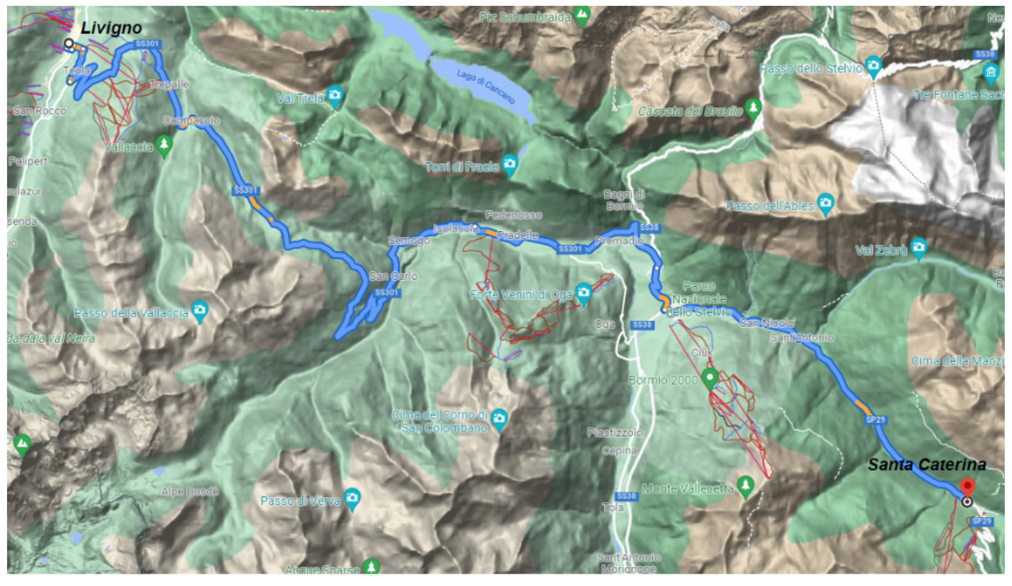
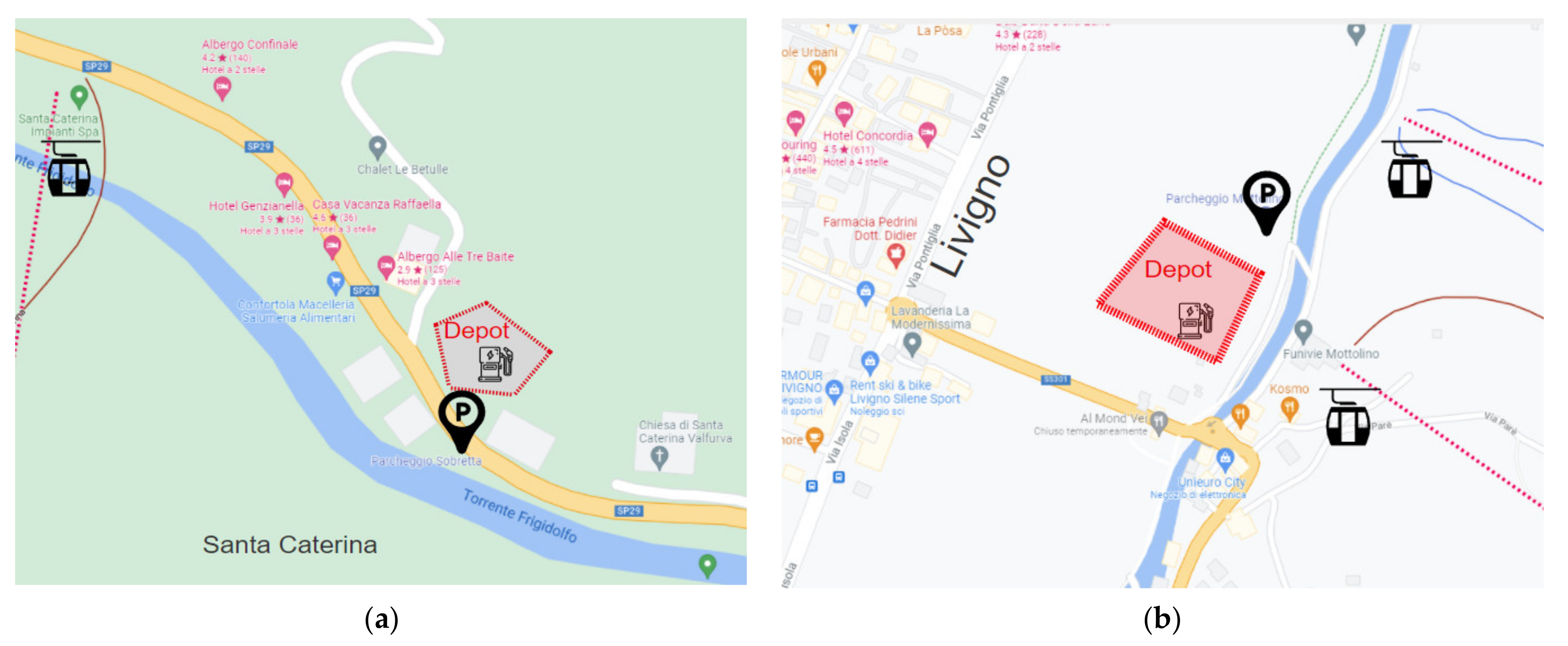
Figure 1 depicts the route that will be analyzed in the paper. The study area is limited to a valley and in particular to Valtellina present in the North Italy—Lombardy region, on the border with Switzerland. It is known for its ski centers, hot spring spas, foods, and wines.

A bus service already existing connects the main spots of interest, it is thus valuable focus on the existing roads and rails sections available for the mobility of public transportation. To assess the energy consumption and hence the motion of the vehicle in the considered sections, we need the geographical and geological attributes of the territory. The elevation profile and all the other data have been remotely acquired with Google Earth and all its features.

2.1. Path Analysis

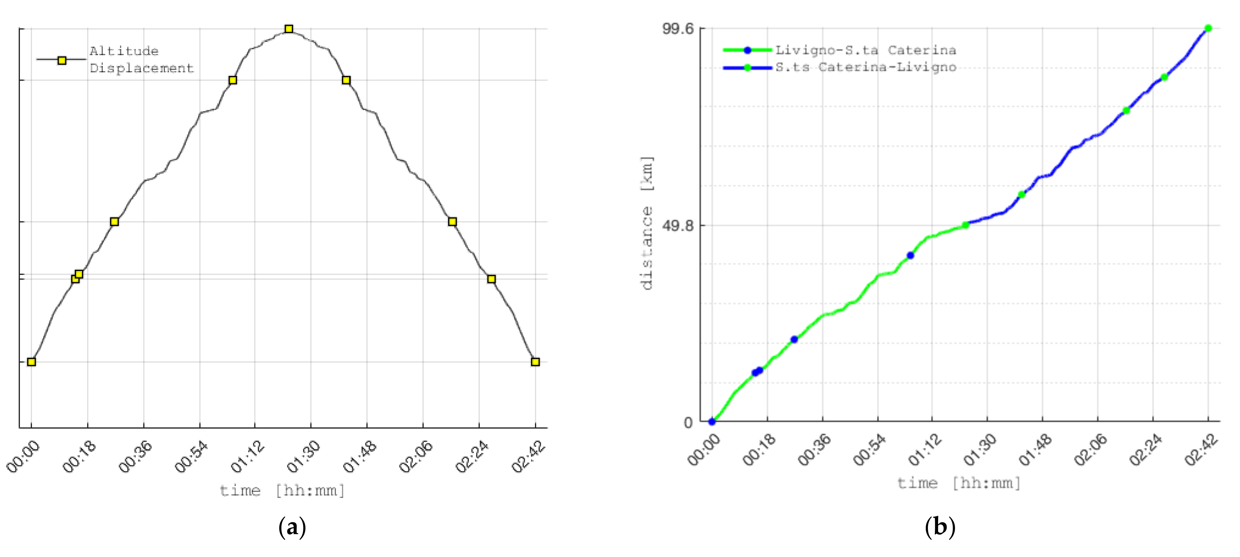
The chosen route is 49.79 km long and a primary segmentation concerns the stops planned, starting from Santa Caterina: Bormio, Isolaccia, Trepalle, Livigno. Here a stop has been included in Bormio where the bus will have to stop is will only be present on the outward journey and will not be present on the return journey. The overall duration of one direction trip is around 1 h and 10 min according to google maps estimation and hence the theoretical average running speed of the bus should be about 43 km/h. A detailed description of the path is reported in

Table 1. Route characteristics.

Santa Caterina—Livigno Altitude
Tract [km]	Average Gradient UPHILL	Average Gradient DOWNHILL	Starting Elevation	Arrival Elevation	UPHILL km	DOWNHILL km
0–5	1.2%	−6.5%	1748	1459	1	4
5–10	1.8%	−4.4%	1459	1286	0.5	4.5
10–15	5.1%	−4.1%	1286	1295	2	3
15–20	3.5%	−2.6%	1295	1382	4.7	0.3
20–25	7.6%	−2.4%	1382	1720	4.8	0.2
25–30	7.3%	−1.8%	1720	2005	4.8	0.2
30–35	7.0%	−3.9%	2005	2276	4.3	0.7
35–40	6.0%	−7.0%	2276	2104	1.3	3.7
40–45	7.0%	−6.5%	2104	1979	1.5	3.5
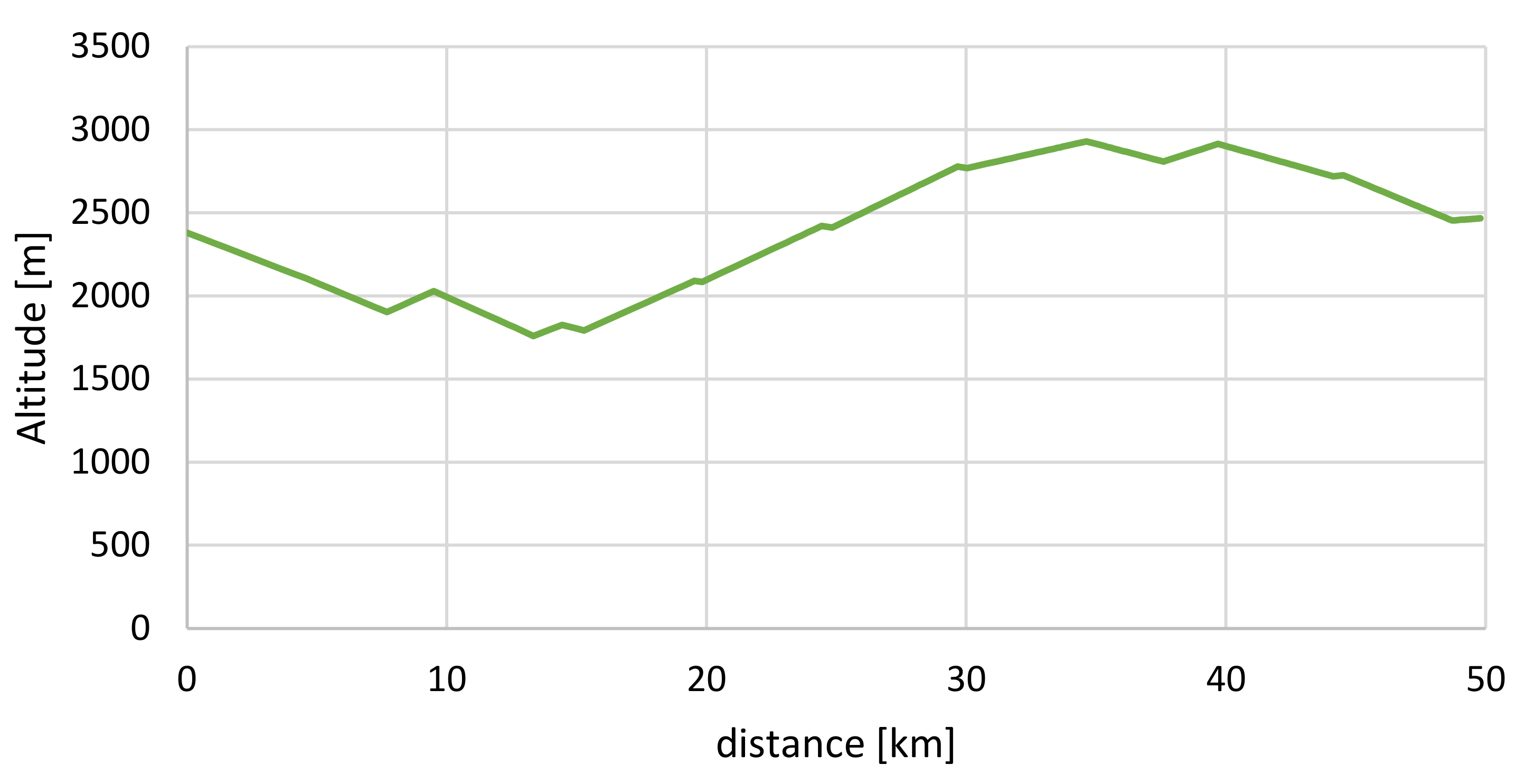
45–50	0.2%	−6.0%	1979	1819	0	5

. The whole path is partitioned on sections of 5 km each where the gradient is computed assuming a succession of climbs followed by descents.

The profile represented in Figure 2 is typical of a mountain environment with an average gradient of 5.8% and a maximum slope of 19%. This is a critical value thus we will have to verify that the chosen bus can overcome it fully loaded. By inverting the direction of travel and then reading the graph backward it is possible to reconstruct the return trip. The drop between the two terminals of more than 600 m reveals the way back is overall mostly downhill. We thus expect the travel time to be slightly less in the inverse direction for an overall duration of a round trip of more or less 2 h.

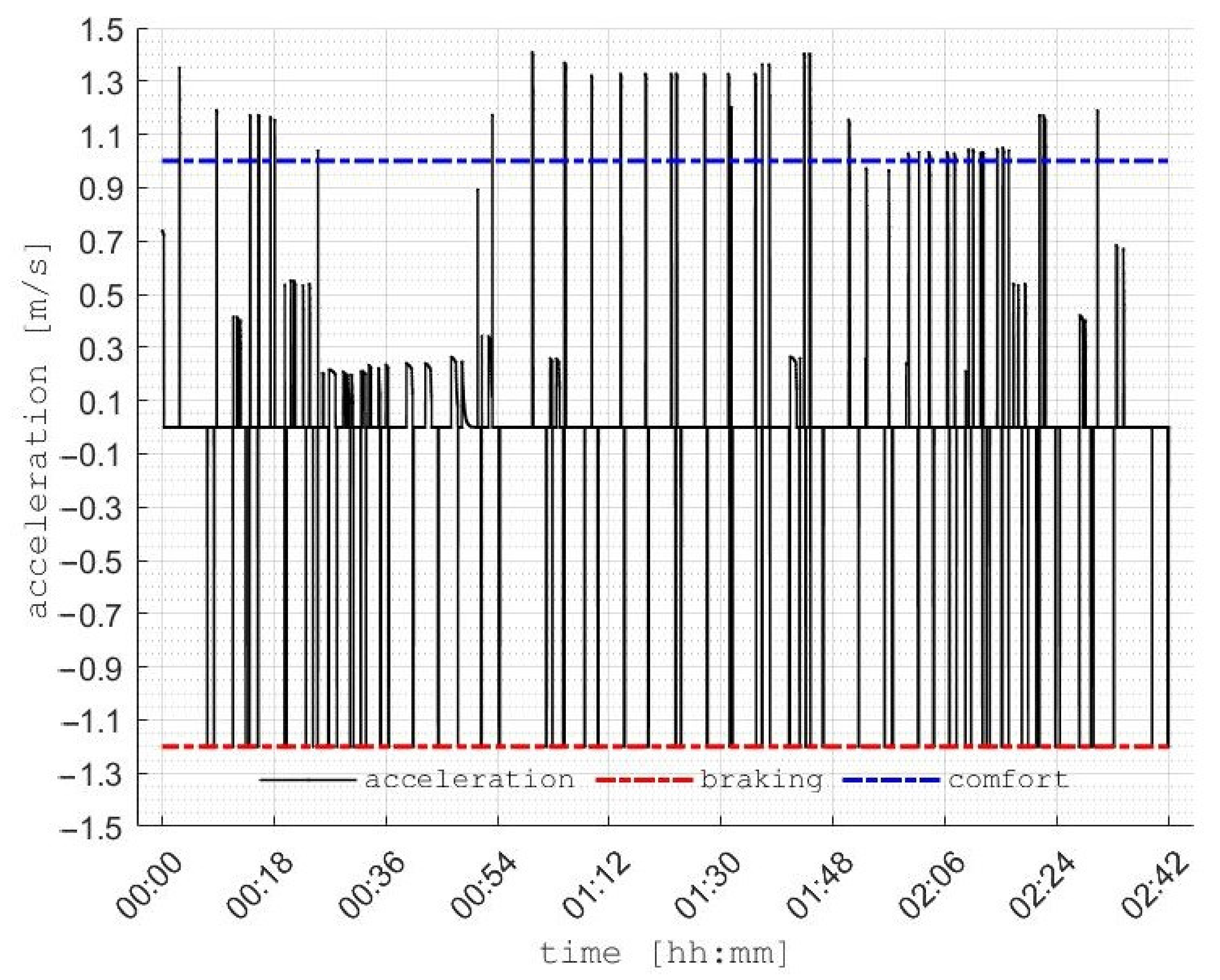
We have created in this primary stage inputs for the future modeling hence the path is divided into linear zones which differ on main physical features. Sharp curves, hairpins, tunnels, and particularly steep sections would determine the different speeds the bus can keep respecting safety and comfort requirements. Practically the zoning clustering is performed according to reference values we manually set. With a qualitative evaluation we sum up in these limit values all the constraints in acceleration the bus will meet along the street:

• Maximum lateral displacement- curving behavior
• Adhesion conditions (avoid slippage)
• Traffic Code limits
• Congestion level

Some assumptions are embedded here for the simulation without introducing more detailed considerations.

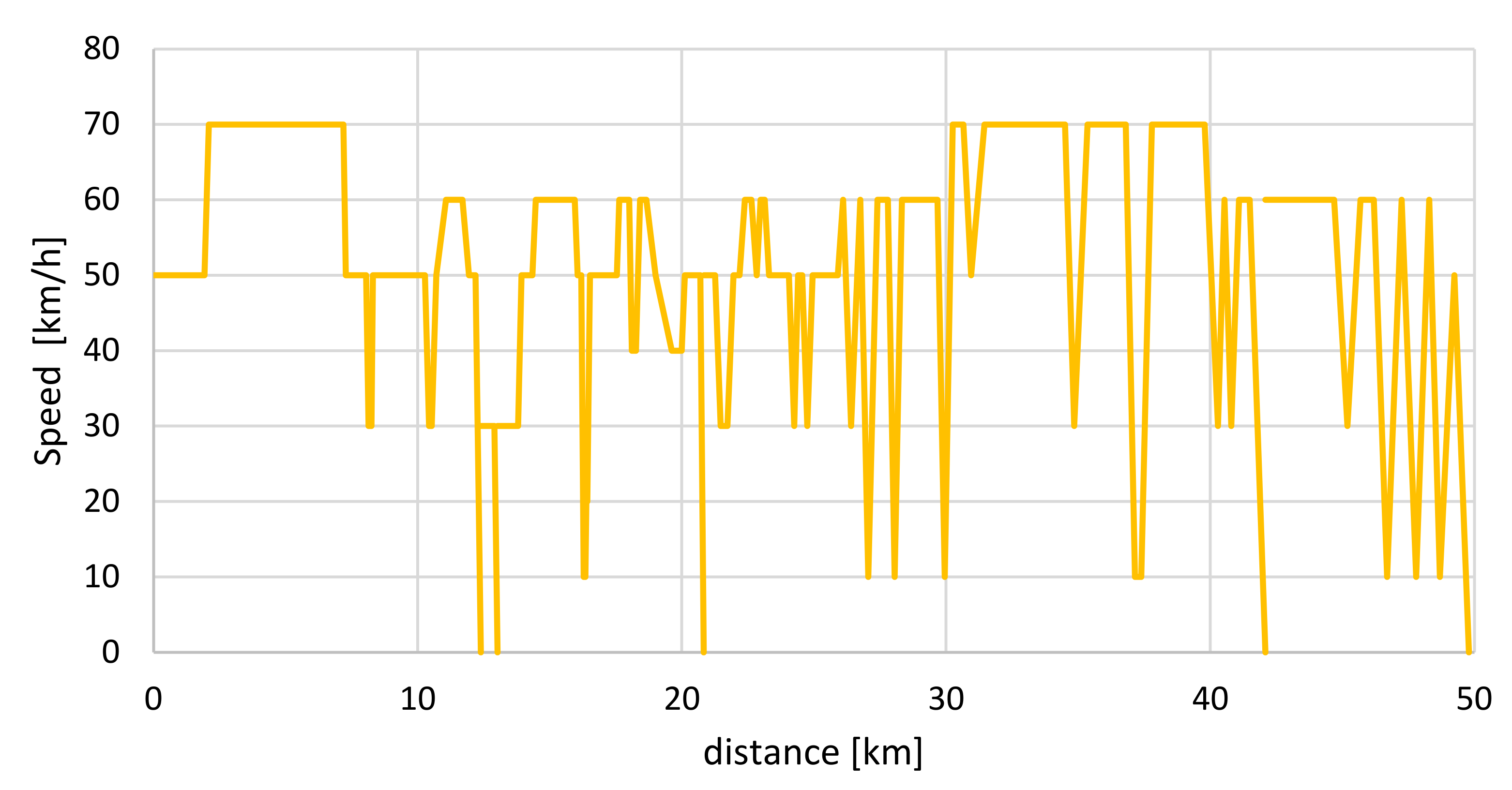
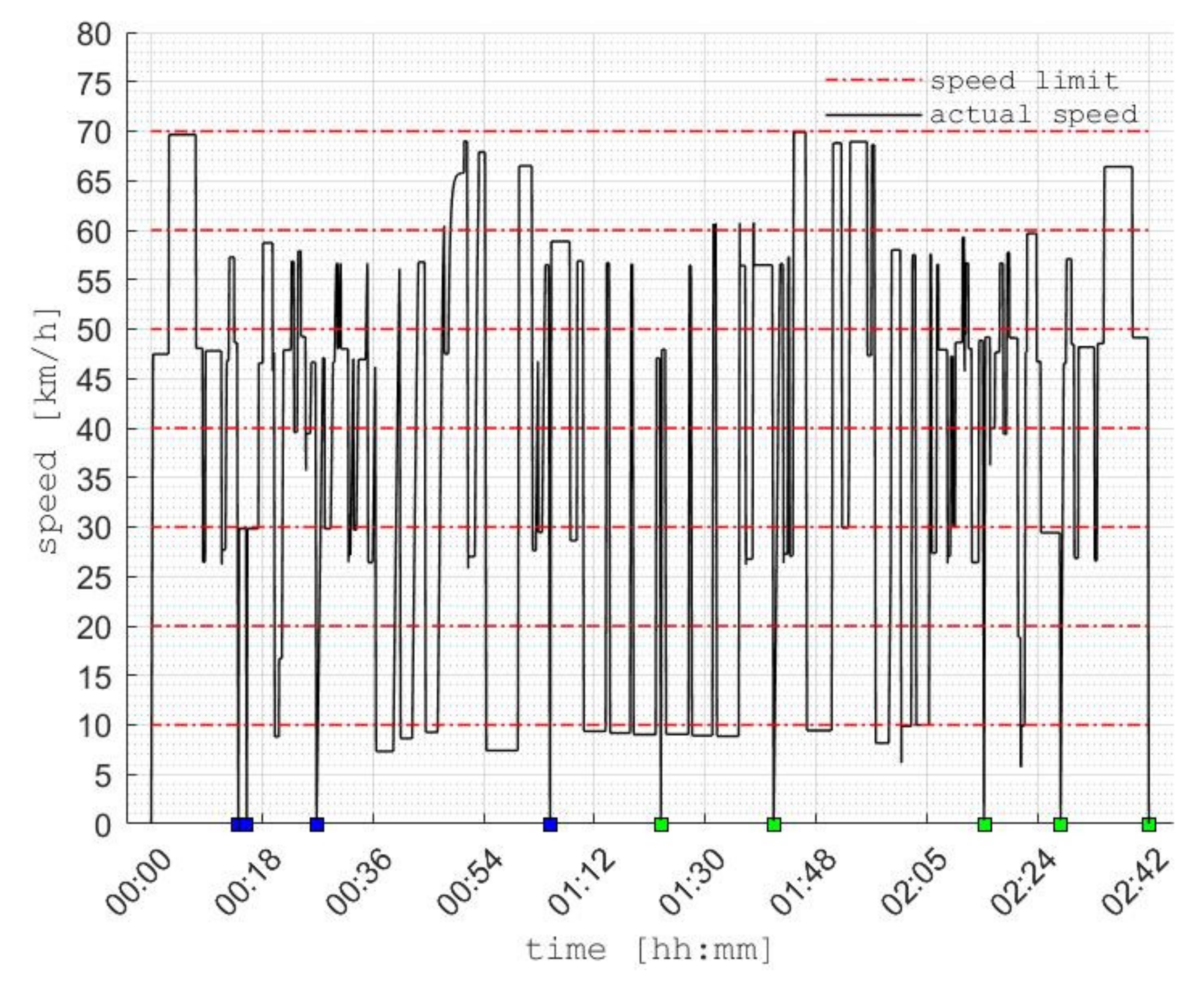
The reference speed profile, depicted in Figure 3, is characterized by assumed instantaneous changes cross successive zones while zero speed is found when the bus is forced to arrest its run.

In the reference speed profile, 7 types of different sections (limits from 10 km/h to 70 km/h) are recognized for the succession of 67 zones. Thereafter all the values are adjusted for the opposite direction. The total travel time at maximum speed comes to be 72 min, the performance is similar to the one revealed at the beginning referring to the online navigator (69 min) we thus conclude the assumptions are realistic ones and can turns, in further chapters into reliable performance estimations.

2.2. Main Issues of the External Environment

To build a reliable electric bus line different factors which influence the operation of such vehicles must be considered. In this specific case, the main difficulties the electric vehicles must face come from the fact that the operation is located in a mountainous and cold environment.

Livigno is located at 1830 m above sea level with an average annual temperature of 3 °C. In the hottest month, 11.4 °C can be reached while in January temperatures around −4.8 °C are reached [10]. Such low temperatures have an impact on the battery; indeed, they can lead to a reduction in autonomy of 20% for diesel buses and about 40% for electric vehicles. This must be considered in the planning phase to properly size the line operation. However, it is crucial not to oversize the line to balance the higher consumption in winter that will reveal an exceeded range availability not necessary during spring or summer.

Another aspect in which there is a strong influence of critical low temperatures regards the behavior of the battery [8,20] and hence of the charging system [9]. Cold weather reduces the chemical and physical reactions happening inside the Li-ion battery, specifically conductivity and diffusivity, leading in this way to:

• Longer charging time (increased impedance)
• Temporary reduction in range (lower capacity)

To avoid this problem the new models of EVs have a thermal management system whose aim is to keep the battery in a safe temperature range to maintain the energy storage capacity, driving range, cell longevity, and system safety [21].

3. Results

3.1. Comparison among Electric Buses on the Market

The selection of the most suitable electric bus to be used in this service is based on the comparison of the electric buses currently on the market.

As introduced in the first chapter, the route under analysis requires some significant constraints within the bus identification. Particularly it is necessary to bear in mind that we need a bus with a certain prefixed minimum range, able to transit through mountain roads hence characterized by a significant degree of gradient and able to corner in sections with a very small curvature radius. Furthermore, since the vehicle must cover about 100 km for a round trip a model with a suitable installed battery capacity should be chosen. Thus, the analysis will be carried among the following four models:

• Mercedes—E Citaro [22]
• Solaris—Urbino 18
• Volvo—7900 Electric [23]
• Proterra Catalyst E2 max [24]

To find the model that best fit the requirements the minimum practicable radius of curvature, and then the cost and the autonomy of each model were analyzed. The width imposed by Italian laws is about 2.6 m and the average height around 3.3 m, while instead, the length can more freely vary. Maximizing passenger capacity of about 120 passengers the Solaris Urbino 18 certainly stands out from the others. However, its huge weight and restricted turning capabilities forced us to remove it from the list and thus figure out a bus with a length of 12 m so that it could still guarantee a capacity of at least 40 people. At this point, the bus with the highest autonomy was carried out. This would allow buying as few buses as possible in the fleet and at the same time save a lot on the infrastructure used for recharging or storing vehicles. Proterra E2 max is the electric bus with the larger autonomy in the world, it can travel more than 400 km fully loaded. On its side Mercedes e-Citaro, despite the interior finishes and advanced charging systems, can travel a maximum of 170 km. Volvo 7900 is the quietest electric bus in the world which justifies a rise in prices in the unit combined to a still lower range of 200 km of autonomy. Thereby mainly in terms of economic convenience, Proterra E2 Max Catalyst has been selected.

3.2. Battery Analysis

Batteries play a fundamental role within electric vehicles. They mostly define the autonomy, charging speed, and lifetime of the vehicle. They also affect the price of the vehicle itself since they are the most expensive component inside an electric vehicle [25].

Lithium batteries can store huge amounts of energy, managing to reach one of the lightest weight-power ratios ever. Among the disadvantages, however, there is certainly the high reactivity of lithium (Li) [26]. Indeed, in the event of high temperatures or fires, they can be led to low-level safety for the vehicle. For this reason, in the design phase, it is preferred to develop an elementary cell system that monitors the battery when underuse. Another outbreak to the implementation on a large scale comes from the relatively high costs of the technology.

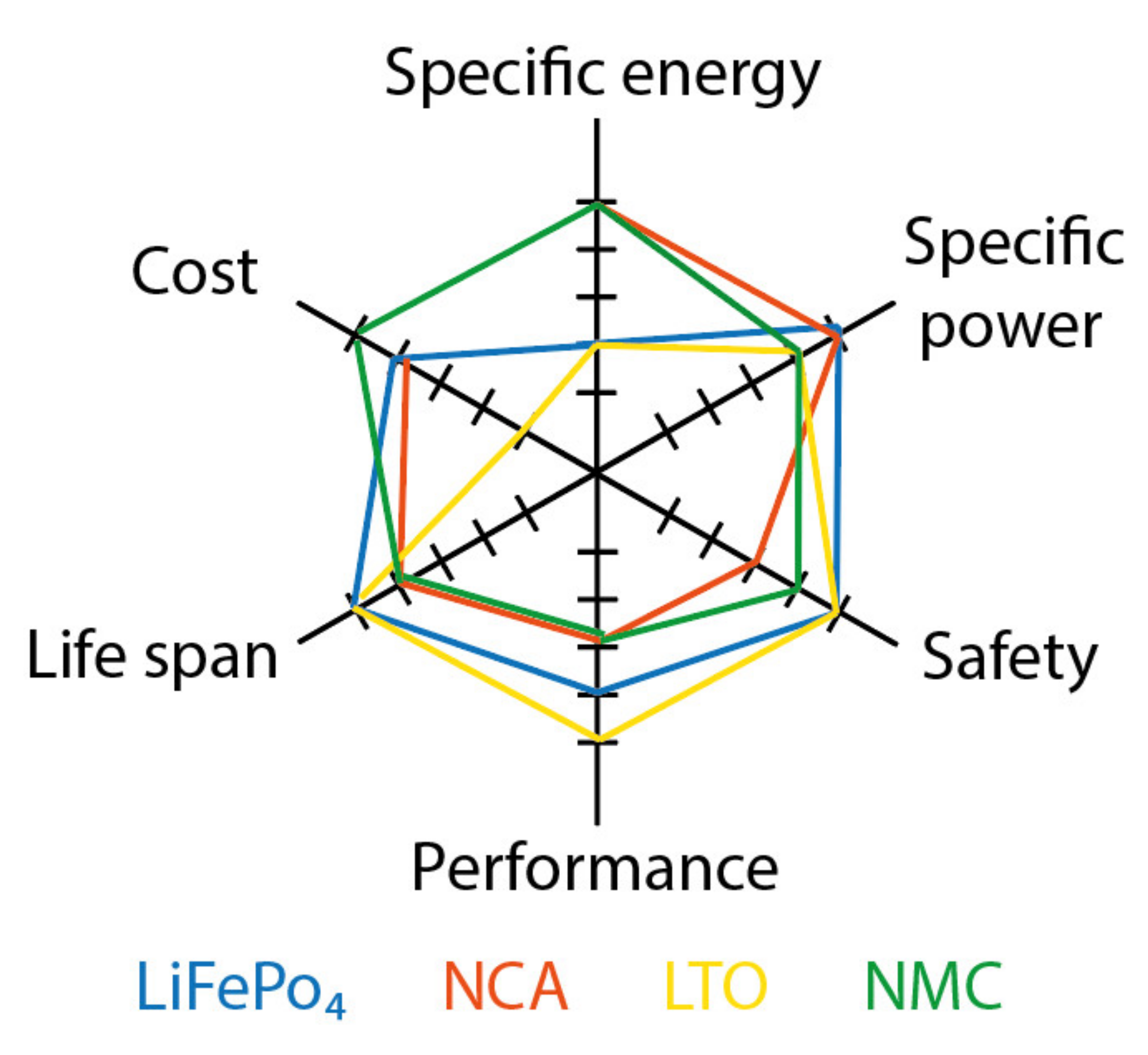
In this type of battery, the materials used for making the cathode, the anode, and the electrolyte can vary defining in this way different lithium-ion batteries technologies [27]. In the following we have analyzed the main candidates for EVs according to the most important parameters:

• Specific energy [Wh/kg]: energy per unit mass
• Cost [€]: investment and maintenance costs
• Lifespan: a measure of battery longevity
• Performance: charging and discharging rates
• Safety: the probability of damaging the surrounding environment
• Specific Power [kW/kg]: power per unit mass

Lithium Iron Phosphate (LiFePo₄): they are batteries with good electrochemical performances and low resistances. They have good thermal resistance and a higher level of safety. They have a high cyclic life (2000+ cycles) and well withstand full charges and discharges. They have a moderate specific energy (100–120 Wh/Kg). Compared to other Li-ion batteries, however, it suffers from a slightly higher self-discharge. Increasingly more lead acid batteries in EV are being replaced by this technology.

Lithium Nickel Cobalt Aluminum Oxide (LiNiCoAlO₂ or NCA): High energy, power density and good lifetime. High cost and marginal safety are negatives.

Lithium Titanate (Li4Ti5O12 or LTO): It is very safe and well resistant to high temperatures. It has a very high cyclical life (3000–7000 cycles) and a low cost. It has the disadvantages of having a low specific energy and power.

Lithium Nickel Manganese Cobalt Oxide (LiNiMnCoO2 o NMC): they consist of a very interesting combination of Ni Mn and Co, within the cathode of the cell. Nickel has a good specific energy but is not very stable, manganese has opposite qualities. This type of battery has high values of specific energy, good thermal resistance, a fair life expectancy and it can provide adequate power to EVs. For these reasons, the NMC battery pack is the most used in the world of passenger transport indeed we find it installed on by Proterra E2 Catalyst Max.

The indicators of each presented battery technology are summarized in Figure 4.

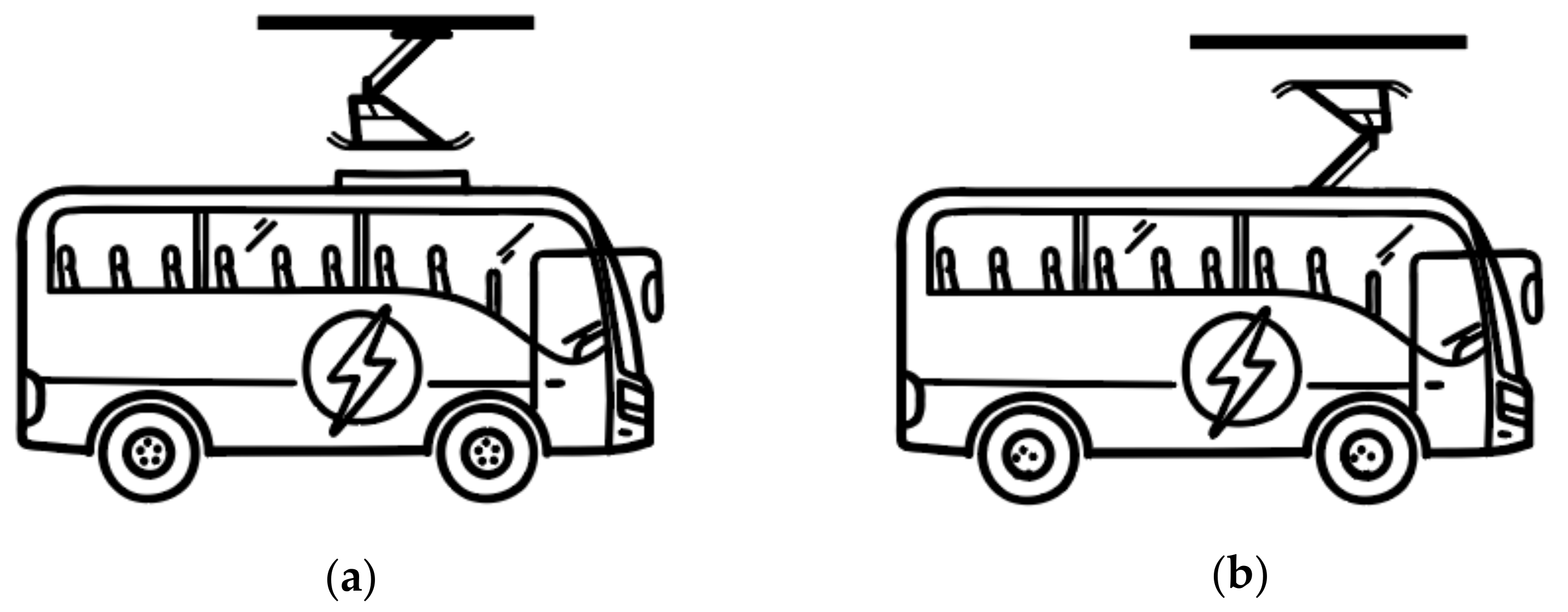
3.3. Characteristics of the Chosen Bus

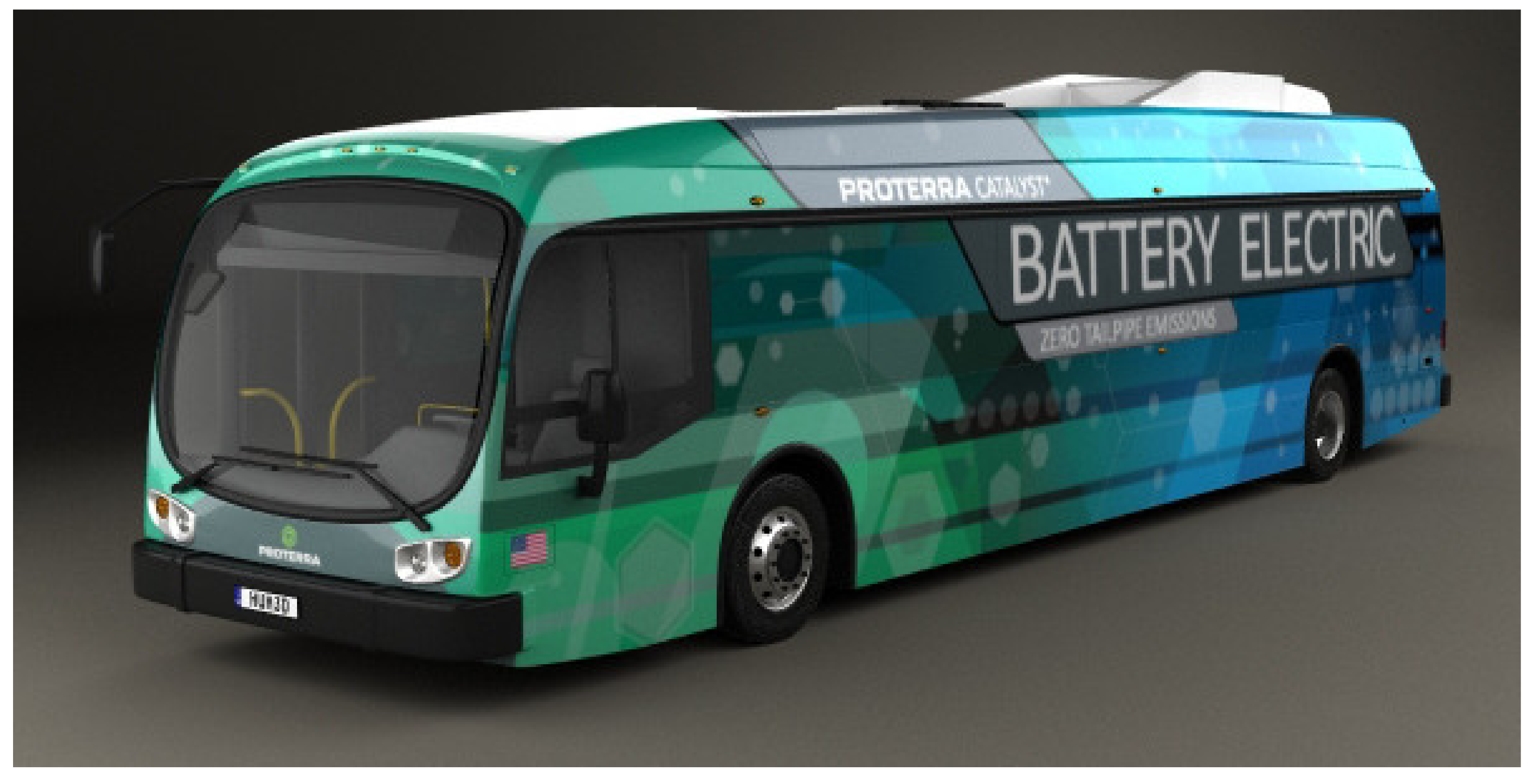
From the previous research, we have identified the Proterra Catalyst E2 max (Figure 5) as the best bus for the purpose, from here onward we will focus the analysis on it. Thus, in

Table 2. Bus technical data.

ELECTRIC BUS DATA
m [t]	19.5	Gravitational mass
me [t]	23.4	Equivalent mass
$\mathrm{Rated}\mathrm{Power}(P_{max}$) [kW]	330
$\mathrm{Rated}\mathrm{Torque}(T_{rated}$) [Nm]	1000
$F_{t_{starting}}$ [kN]	23.4	Starting tractive effort
$v_b$ [m/s]	14.1	Base speed
$a_{max}$ [m/s2]	1	Acceleration for passengers’ comfort
$a_{BR}$[m/s2]	1.2	Braking deceleration
$B_{el}$ [%]	45	Percentage of regenerative braking
$P_{aux}$[kW]	22	Power of auxiliaries
${\eta }_t$	0.85	Tractive efficiency
${\eta }_b$	0.85	Braking efficiency
$f_{admax}$	0.6	maximum adhesion coefficient
$F_{admax}$ [kN]	114.777	maximum adhesion limit
Frontal surface [m2]	6.936
$C_x$	0.6	Bus shape coefficient [28]
Air density [kg/m3]	1.225	Air density at 15° at sea level and 1013.25 hPa.

are reported in detail its technical characteristics which affect forthcoming results.

Some of these data were directly taken by the datasheet provided by the manufacturer [24], others, such as the percentage of regenerative braking, were estimated starting from the values present in the literature.

In estimating some parameters, we stressed the specificity of the route (i.e., the extreme conditions of temperature and slope). For example, the value set for the power consumption of the auxiliaries ${\mathrm{P}}_{\mathrm{aux}}$ is quite high so to perform the analysis in the worst-case scenario, that means with intense use of heater and other ancillary devices indicates the electric power absorbed by auxiliaries, which has been considered equal to 22 kW [29].

The parameters ${\eta }_t$ and ${\eta }_b$ identify the efficiency in the traction and braking phases, respectively, while $B_{el}$refers to the maximum percentage of energy recovery during the braking phase. The energy recovered during braking has a high influence on EV energy consumption and its value is strongly influenced by the mean vehicle and by the applied deceleration. According to [29], for a bus operating in an urban context, the value can be assumed about 45%.

Further clarifications should regard the value of the maximum adherence coefficient $f_{ad\_max}$. It strictly depends on the condition of the road and the type of tires; thus, we selected a quite low value that is between the thresholds of dry and wet but good conditioned tarmac.

4. Simulation of the Motion of the Bus

4.1. Methodology

In order to practically simulate the movement of the vehicle, the values of the acceleration a and of the tractive effort $F_t$ are controlled, according to the motion equation expressed in (1):

$$F_t-\sum R=m_{e}a$$

(1)

where R involves all the resistant forces which oppose the forward motion of the vehicle and $m_e$ is the equivalent mass.

Based on the value of the tractive effort $F_t$ and of the acceleration a, the vehicle can operate in manly four different operation modes.

• Powering mode. In this mode, the tractive effort is higher than the sum of all the resistances and hence the vehicle undergoes an acceleration.
• Braking mode. During the braking of the vehicle a negative tractive effort is applied (braking effort can be applied by the motor or the braking system) and hence the vehicle decelerates.
• Free-running mode. In this mode, the tractive effort is enough just to overcome the resistances ($F_t=R$) that oppose the forward motion of the vehicle and hence this latter will proceed at a constant speed.
• Coasting mode. Lastly, if $F_t$ is nil, then the bus naturally decelerates because of the contribution of the resistances.

Considering that the operational performance of the bus has limitations both in structural terms and from external factors that cannot be overcome for safety reasons we report below:

• Reference speeds and speed limits are set and described in Figure 3.
• Adhesion of the wheel: the maximum force which would avoid slippage phenomena is computed considering the current speed and the transient of the engine.
• Passenger comfort: with the aim of a rightful level of onboard comfort the braking deceleration is sought not to exceed the value of $1.2\frac{m}{s^2}$.

The operating conditions shown above are the inputs that model vehicle traction and will be part of the MATLAB simulator. Indeed, correspondent indicators ensure the thresholds are met throughout the entire simulation.

Finally, to simulate the vehicle motion we have to compute the resistances to the motion R. The motion of a bus is resisted by mainly four forces which are: the inertial force, aerodynamic force, resistance due to the grade, and rolling resistance [6]. To consider the inertial resistance of the rotational elements inside the vehicle the concept of equivalent mass $m_e$is considered. The equivalent mass, computed in (2), is the static mass (m) of the bus increased by a coefficient β at which is assigned a value equal to 0.2 in this specific case.

$$m_e=m·\left(1+\beta \right)$$

(2)

The formulas used to compute the air, the grade, and the rolling resistances are reported from (3) to (5), respectively.

$$R_{air}=\frac{1}{2}·\rho ·A_f·c_x·v^2$$

(3)

$$R_g=m·g·\sin \theta$$

(4)

$$R_r=m·g·f_v·cos\theta$$

(5)

The air resistance (3) depends on the air density $\rho$, the square of the bus speed v, its frontal area $A_f$, and on a shape coefficient ${\mathrm{c}}_{\mathrm{x}}$. Instead, the grade resistance depends only on the slope $\theta$ and on the vehicle mass m. Finally, the rolling resistance is related to the mass m, to the slope $\theta$ and to a rolling resistance coefficient $f_v$.

4.2. Analysis and Discussion of Results

This paragraph explains the outcomes of a round trip along the considered path. In Figure 6a,b are given the space profile respectively qualitatively and quantitatively.

The overall returned trip takes about 2 h and 42 min; taking 1:23 uphill and 1:19 downhill. As we assessed at the outset one direction is slightly faster since there is a drop in altitude between the two terminals. The total distance travelled is around 99.6 km exactly split in half as the bus walk the same path in both directions. This means the blue and red lines are symmetric. The assumptions of the developed study do not include ancillary time and lasting breaks within the journey, they are simplified or embedded on other parameters.

The commercial speed $v_{com}$ of the vehicle is computed (see

Table 3. Commercial speed calculation.

Stops number	8	-
stopping time at the stations	1.5	min
Operation time	162	min
Overall time on the path	174	min
Covered distance	99.4	km
Commercial speed	34.34	km/h

) using the following formula reported in (6):

$$v_{com}=\frac{s_{tot}}{\sum t_t+\sum t_0}=\frac{s_{tot}}{T_{tot}}$$

(6)

where $s_{tot}$ is the overall space and $T_{tot}$ is the complete running time along the path which includes: $t_t$ which is the time interval when the vehicle is in motion and $t_0$which refers to all stopping times. Applying (6), the commercial speed results in 34.5 km/h.

The final velocity profile of the bus obtained from the model is shown in Figure 7.

The horizontal lines respectively indicate the choices made in the speed profile where the maximum recorded speed is 70 km/h.

Figure 8 shows the acceleration profile where we show a negative reference that comes in at −1.2 m/s². In fact, in the model, a constant deceleration is used. On the other hand, as far as the positive acceleration is concerned, it can assume different values in time. The maximum values are recorded at around 1.3 m/s².

Finally, the most important value for correctly sizing the operation of the service is calculated in Figure 9. The simulation and the results obtained are used to evaluate the energy consumption. This analysis is aimed at evaluating the operating costs of the tender, studying the most suitable charging solution, and finally sizing the service and designing the infrastructure.

The value of efficiency during the traction phase has been set at 85% and the remaining 15% is lost in the form of electrical or mechanical losses. The battery not only provides the energy needed for movement but is also responsible for powering all auxiliary services of the vehicle that can draw 22 kW. For this study, the maximum auxiliary energy consumption of the bus was considered.

Another important advantage of electric vehicles is the ability to regenerate energy during deceleration phases, taking advantage of so-called regenerative braking. This feature is particularly important in electric buses since they have heavy mass, fixed paths, and many stop-and-go phases [21]. According to the literature, if regenerative braking is well employed, the amount of recovered energy can range from 40% to 75% [22]. In this study, its value was set to 70%. However, in the model, regenerative braking is not considered when the bus is traveling at less than 10 km/h [23]. By setting all of the above parameters and values in the MATLAB model, the energy required for the bus in order to complete a round trip results in 251 kWh.

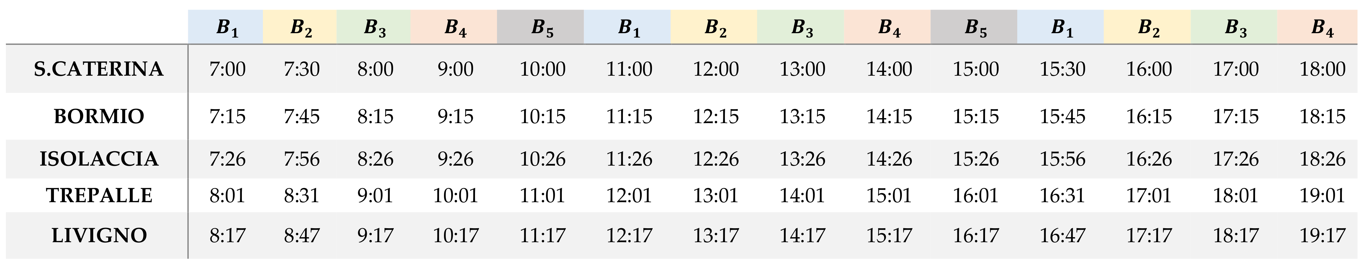
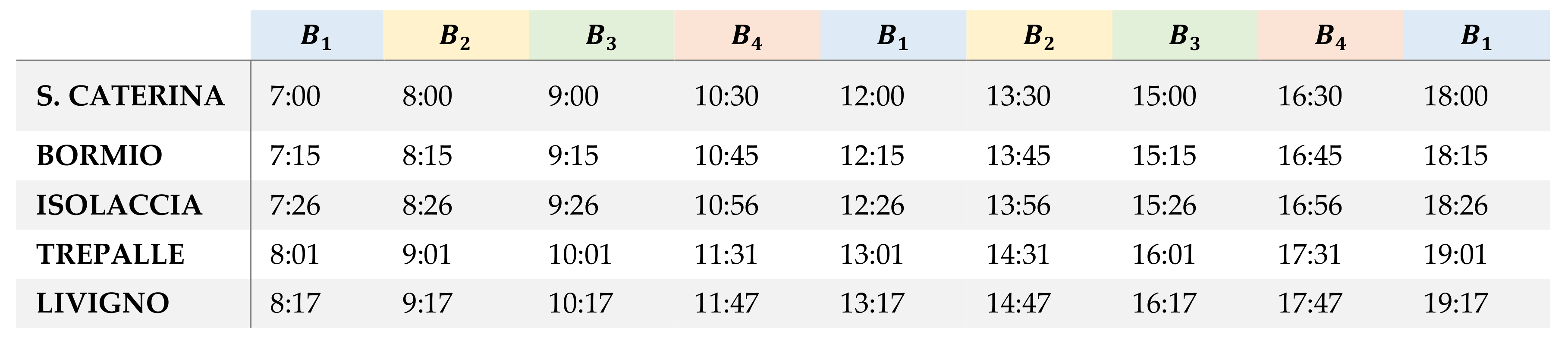
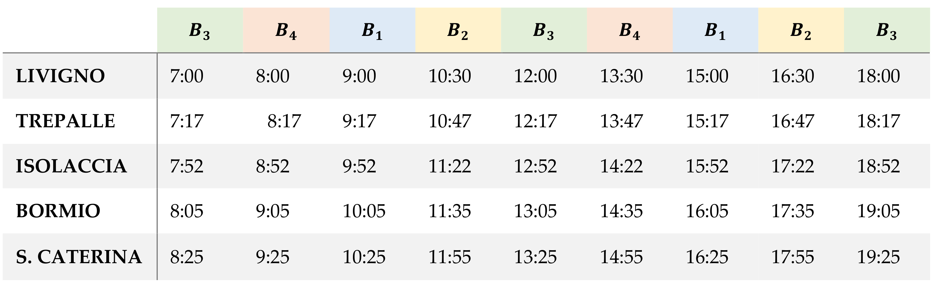
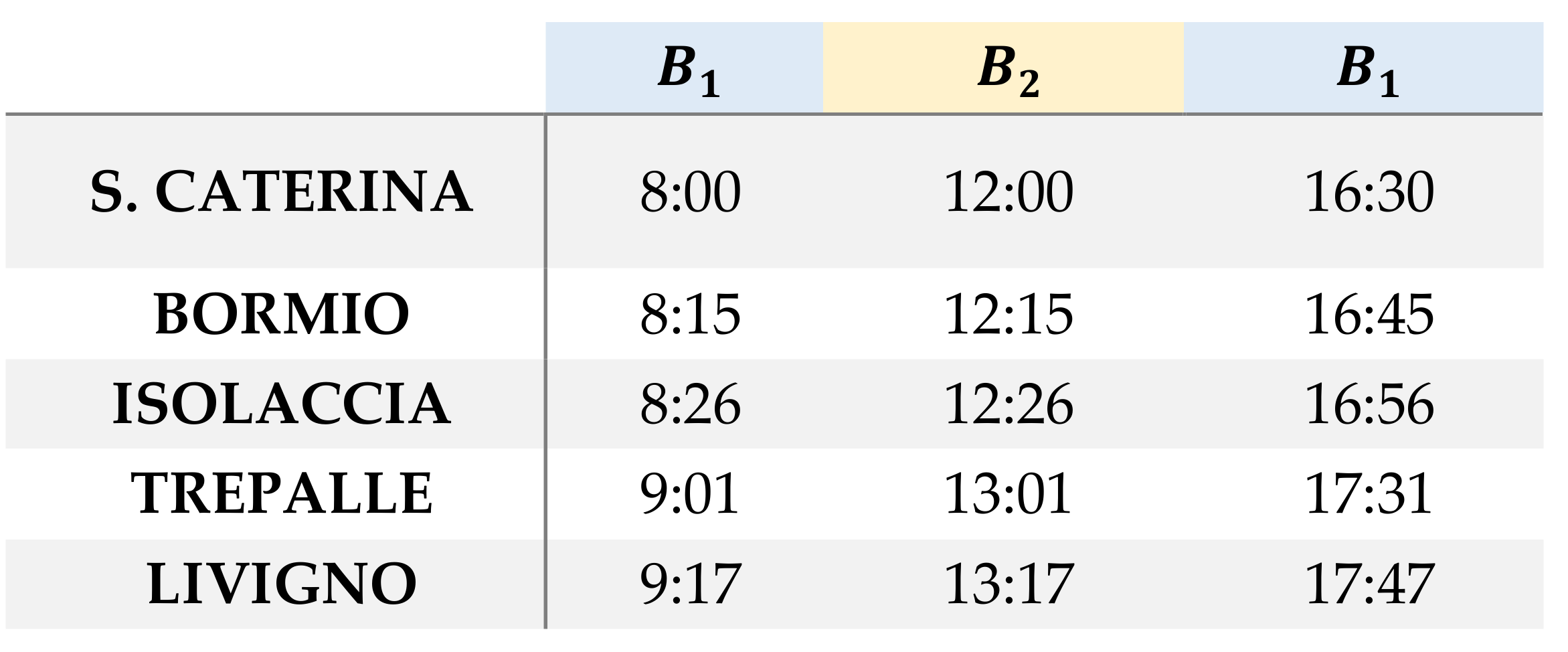
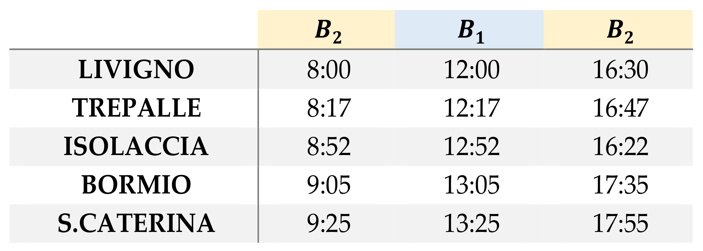
5. Timetables

Buses make a fixed, predetermined number of kilometers every day (i.e., the route is always the same), therefore it is easy to plan stops and forecast travel times. A line timetable is required to provide the service and it is also important in order to understand how many buses will be needed as well as the necessary timing for recharging. To build the timetable three different trends are considered since the number of passengers varies during the year. The high season includes December, January, February, and August; the mid-season includes March, July, September, and November, and the low season April, May, June, and October. The timetables are shown below, from Figure 10, Figure 11, Figure 12, Figure 13, Figure 14 and Figure 15, together with the distribution of buses ($B_i$) allocated on the specific runs.

High season. The service will provide 14 rides/day per direction. There will be one ride/hour plus a couple of rides in the morning and in the afternoon to supply the demand during the peak hours. For this type of schedule are needed 5 buses; $B_1$, $B_2$ and $B_4$ will cover 6 rides/day for a total amount of 290 km travelled while $B_3$ and $B_5$ will take 5 rides/day which corresponds to 240 km. According to the Italian law related to the driver rest hours management, after 4 and a half hours of driving the driver must take a break of at least 45 min. This can be divided into 2 breaks of 15 and 30 min. Therefore, the number of the required drivers must be chosen keeping in mind the just mentioned law. However, from the proposed timetables it can be seen that the rest of the drivers are always respected in each of the five buses.

Mid-season. In the middle season, there will be 9 rides/day per direction. The races will be fewer during the day, more frequent in the morning and the afternoon. 4 buses are needed for this type of service and in particular $B_1$ and $B_3$ will cover 5 rides/day (240 km), while $B_2$and $B_4$ 4 rides/day (192 km).

Low season. For the last four months, just 2 buses are required, the rides will be only 3/day per direction, distributed during the whole day. Each bus will take 3 rides/day for a total amount of 145 km. Seen the low number of trips during the low season, the drivers related to this service could be used also for driving other bus lines or for other services related to the public transport.

For each stop, we set a stopping time of 1.5 min to allow passengers to get off and on the bus. This is estimated to be the worst-case scenario in terms of stop intervals, indeed during the winter season ski equipment and high affluence can lead to long necessary times for boarding procedures.

To conclude it can be said that to provide the wanted scheduled service five electric buses must be bought. All the five buses will operate in the high season, instead in the middle season, the operating buses pass to four and the remaining one could be used as backup bus in case of failure of one of the operating. Finally, in the low season, just two will run and the other three can be used as backup or in other lines or for other purposes. During the high season as backup service, conventional buses already in use for other lines can be employed in case of need, so that the cost related to the purchase of electric buses is not further increase.

6. Charging Infrastructure

The electrification of buses has several operational advantages among which the most relevant can be indicated as follows:

• lower fuel costs due to higher well-to-wheel efficiency,
• less maintenance due to fewer mechanical parts and less vibration,
• a longer expected lifetime compared to the 10–12 years of diesel buses.

However, considering the infrastructural aspect, switching from a traditional vehicle to an electric would require building a well-integrated infrastructure such as bus depots, for example having to introduce a charging system to recharge the batteries of EVs when they are stopped overnight. Several solutions can be found on the market that can be used to address this issue. In fact, the right choice of charging option is relevant in the implementation of a public transport service. It is not possible to define a priori the most performing way to recharge a fleet of electric buses for all situations; the characteristics of each service and each route must be considered to propose a preliminary design. In the following, the recharging system is designed according to the energy consumed by each bus and the number of buses needed to cover all the trips in the timetable.

6.1. Electric Bus Charging Solutions

The charging systems used so far to feed the batteries of electric buses can be split into two main groups:

• Overnight charging: it aims to charge the fleets of electric buses during the night when they are stopped at the depot with plug-in connectors and charging power for each connector from 40 up to 120 kW [30].
• Opportunity charging: it is a super-fast charging system, which is used to recharge the batteries of buses along their routes, located in significant points such as bus stops or terminals, at power ratings up to 600 kW, mainly using over-head pantographs. In particular, concerning this latter component, we can have two different installation choices. In the Top-Down solution (Figure 16a), the pantograph is steadily attached to the charging station, and it lowers on the electric bus once the vehicle is positioned under the pole. The main advantages of this type of installation are listed in the following. First, it has a minimum impact on the bus passenger capacity, indeed on the bus in this case must be mounted just the four connector rails, which weigh 15 kg instead of about 100 kg of the pantograph itself [31]. Then if the pantograph is connected to the charging pole it is not exposed to vibration and weather in the way a roof mount would be. Finally, a pole-mounting solution minimizes the required number of pantographs for a given bus route, and hence it reduces the overall cost for the charging equipment. However, the worst drawback is that in case of failure, the entire line would be affected. Vice versa, in the Bottom-Up pantograph solution (Figure 16b), the pantograph is mounted on the roof of the bus; it rises thanks to a spring mechanism, and it is lowered down to its standard position by an electric actuator. Generally, the alignment between the pole and the pantograph is made through laser guidance for both solutions.

Since opportunity charging technology involves much higher charging rates it can require less energy capacity to be stored in the bus, which could significantly reduce the capital costs of this type of vehicle. However, the cost of the required infrastructure remains very high compared to the overnight charging infrastructure. The use of one charging solution does not exclude the need and the use of the other. As a matter of fact, the charging infrastructure of the electric bus fleet can rely on the presence of both charging systems. Both the solutions have their respective advantages and disadvantages.

6.2. Charging System Proposal

In order to meet the scheduled trips and the energy needs of the planned bus fleet it is necessary to install both in S.ta Caterina and Livigno (both bus stop terminals): two DC charging columns with a power of 150 kW each and finally an opportunity charger with a nominal power of 350 kW. With this planning, all buses can be fully recharged overnight at the depot thus starting service with 100% SoC. However, if needed they can also take advantage of the opportunity to recharge during dwell time. Thus, the new electric skibus line would require the provision of new space to build its depot and charging system. Therefore, the placement of these new depots (ollocated near parking lots that can be used by users as Park&Ride facilities) was designed to be strategically optimized and have low visual impact (Figure 17).

7. Electric vs. Diesel Bus

In this paragraph, the performances of the electric bus fleet are compared with those of a diesel fleet both in terms of emission and cost savings.

For this comparison, we have selected the diesel bus Serta Multiclass S 415 LE business (Figure 18). We have selected this specific bus since it is similar in terms of capacity and physical characteristics (i.e., length and weight) to its electric competitor: the Proterra Catalyst E2 max.

7.1. Fuel Costs

Another, and perhaps more interesting yardstick for comparison between the two alternatives is the fuel cost. As mentioned in the first section of the chapter there are a lot of parameters that influence the energy consumption of a vehicle in general; however, for the sake of simplicity, for this analysis, we will assume that the ICE bus and the EV require the same amount of energy, thus equal to 251 kWh for each round trip. Let us start with the older and less eco-friendly ICE bus. The energy necessary to the motion, in this case, comes from the combustion of diesel. The heating value and the average cost of this fuel are reported in

Table 4. Diesel specific values.

Diesel Specific Values
Heating Value [J/kg]	42,700,000
Density [kg/l]	0.835
Price [€/l]	1.29

.

The fuel mass flow rate necessary to generate 251 kWh of energy is computed in (7) and (8), where $F_t\left(i\right)$ is the tractive effort in each instant of time i, $v\left(i\right)$ is the forward speed, ${\eta }_{diesel}$ is the efficiency of the diesel powertrain and $P_{aux}$ is the power absorbed by the auxiliaries which rely on the combustion of the fuel as well. Summing up the mass flow rate over each instant of time (discretized in seconds) we later got the overall mass of diesel burnt in a single round trip. With the specific density of diesel $d_{diesel}$ is then derived in (9) the necessary volume of diesel in liters $V_{comb}$. 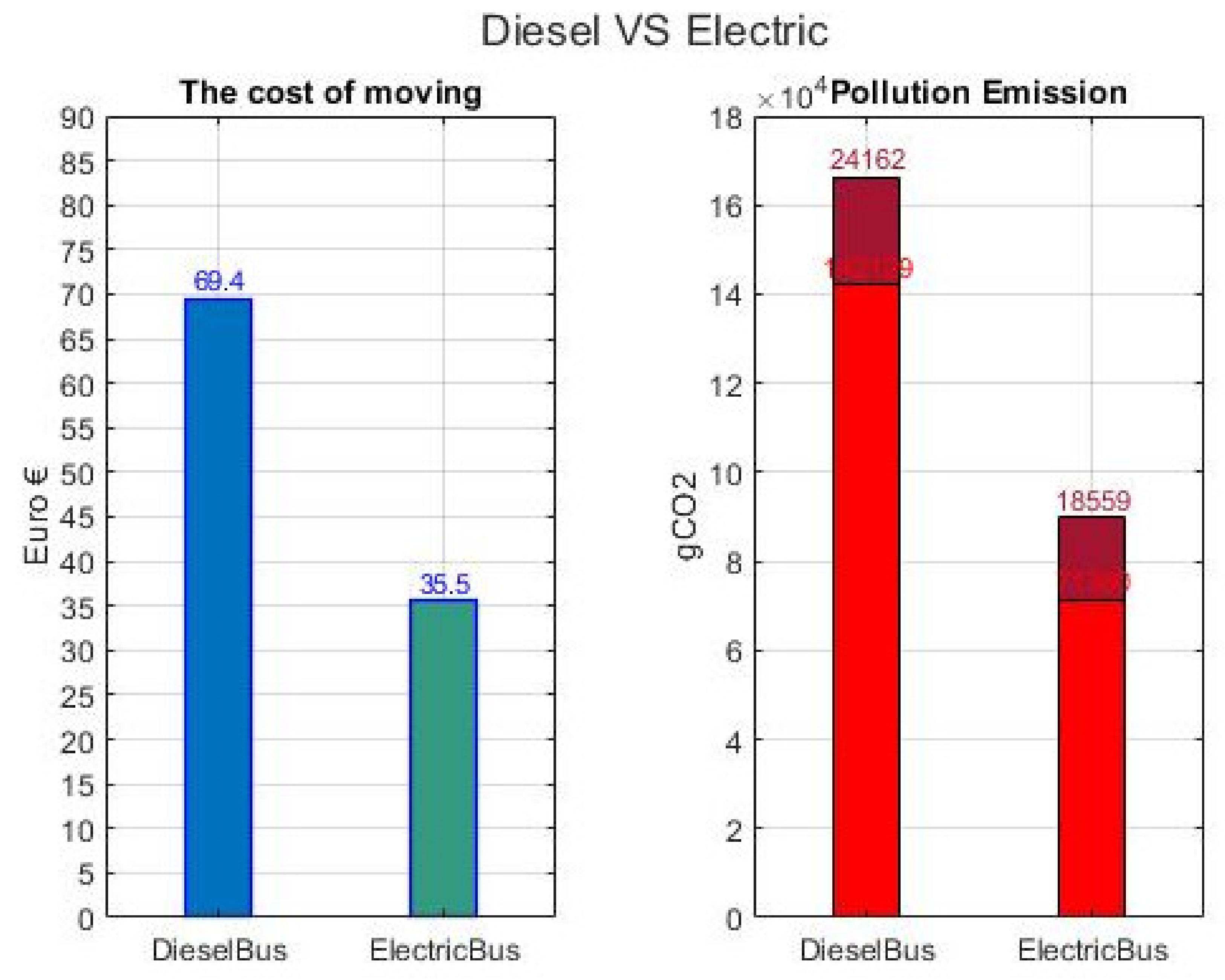Finally, in (10) by multiplying the required liters of fuel by its price the overall fuel cost to move the first bus on the route is found and it turns out to be equal to 69.45€.

$$m_{comb}\left(i\right)=\frac{\frac{F_t\left(i\right)·v\left(i\right)}{{\eta }_{diesel}}+P_{aux}}{Heating valu{e}_{diesel}}·1000$$

(7)

$$m_{comb}=\sum m_{comb}\left(t\right)$$

(8)

$$V_{comb}=\frac{m_{comb}}{d_{diesel}}$$

(9)

$$Tot cos{t}_{diesel}=V_{comb}·Pric{e}_{diesel}$$

(10)

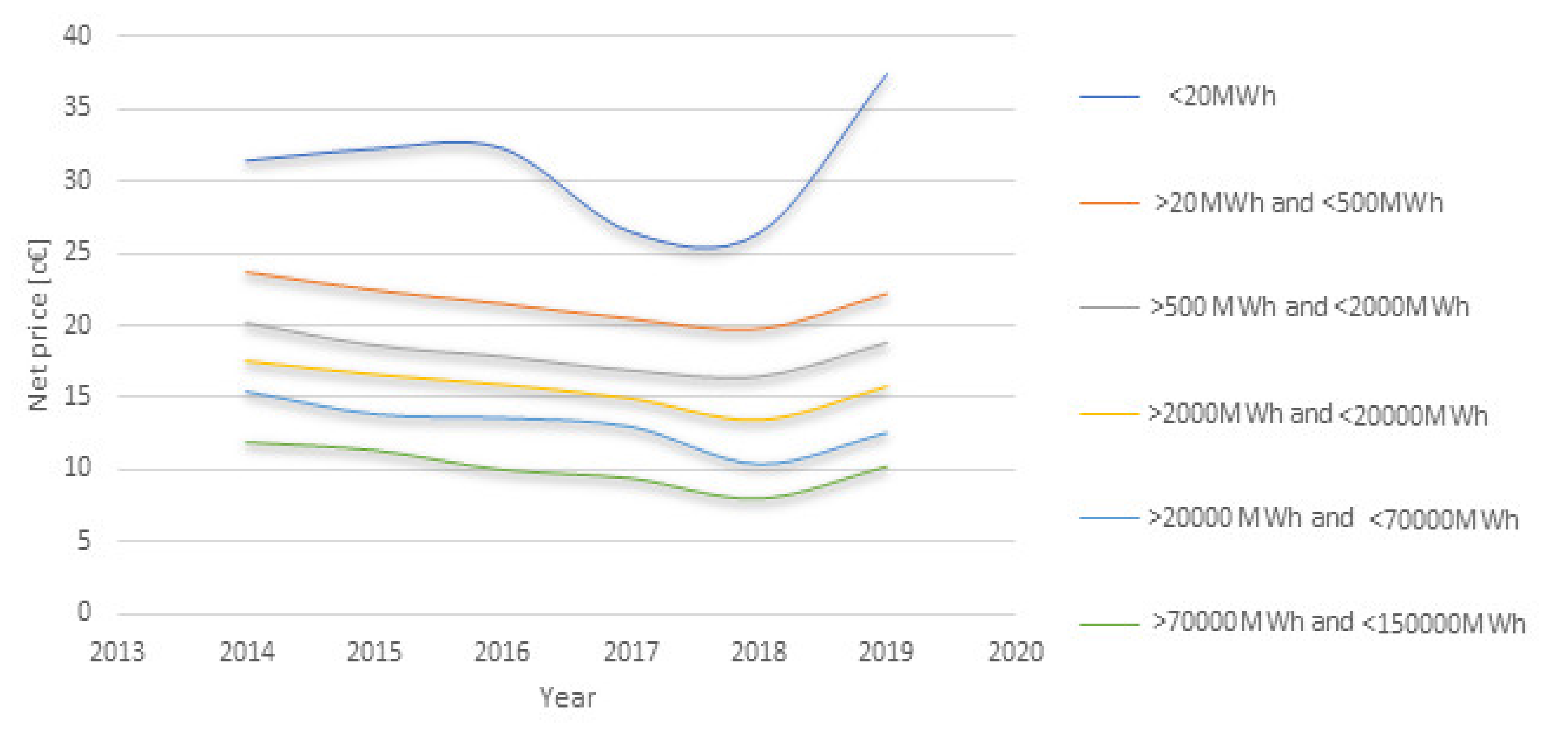
In the case of the electric counterpart, the computation is easier and directly the product of the flat cost of electric energy per kWh and the total amount of energy considered. The key point here is the price of electric energy itself.

Figure 19 shows the trend of the electric energy price in the last six years based on the annual consumption class [16].

As can be seen, the differences are tangible scaling from one class to another; hence, it is essential to understand which one referring to for our service. The resulting energy consumptions per year is about 813,240 kWh/year (251 kWh × 3240) therefore we have to relate to the grey range in the graph. The prices used for these calculations and represented in the following plot are the ones aimed at a company with a VAT number. Considering the fact that the energy is for a public service we supposed that our company could receive a discount of the 50% of the taxes reaching a final price of the energy of 0.1412 €/kWh. We can finally conclude the analysis of the fuel costs calculating the cost of a round trip for the electric bus that results in 251 kWh × 0.1412 €/kWh = 35.44 €: half of the cost for a diesel bus.

7.2. Operational Emissions

To determine the emission of a vehicle it is important to consider its full life cycle. The objective of the Cycle Life GHG (Greenhouse Gasses) is to analyze all emissions produced in the construction, use, and disposal of the vehicle, a Bus in this case. Many studies try to compare the lifecycle GHG emissions of EVs and ICEVs [32,33], but they usually give very different results. It is difficult to understand the reliability of these studies because often the data is not sufficient to understand the complete path of every single component of the vehicle, from the production to the assembling and its disposal. We will not deepen the Cycle Life GHG analysis. Indeed, for the comparison between an ICE Bus and a Battery Electric Bus, we will take into consideration only a part of it, by studying the emissions caused by the operation of the vehicle.

Diesel Bus: in the Well-to-Tank emission of diesel fuels we take into consideration the crude oil extraction, overseas transportation, petroleum refining, and domestic transportation as reflected in

Table 5. Emissions related to Diesel Cycle [34].

	Conventional Diesel [gCO2/kWh]
CRUDE OIL EXTRACTION	2.74 (Operation)
	1.37 (Flare Combustion)
	1.19 (Associated CO2)
	0.14 (CH4 vent)
OVERSEAS TRANSPORTATION	3,31
PETROLEUM REFINING	9.58
DOMESTIC TRANSPORTATION	1.33
FUELING TO VEHICLES	0.00
TOTAL	19.66

.

The emissions of the Well to Tank can be assumed as 19.66 [gCO₂/kWh]. The total for our trip is then 4919.6 [gCO₂].

For the Tank to Wheel analysis, it is assumed that potentially, if its efficiency conversion is assumed 100%, the diesel combustion leads to 270 g of CO₂ for every kWh produced. So, for our trip, considering the efficiency of the diesel motor by about 33%, the total annual emissions are calculated as 665.3 [ton CO₂]. The total CO₂ emissions for the diesel buses in our path would have been equal to 210.3 [kg CO₂] for a round trip.

It is important to understand that the emissions produced in this phase are “direct”: they emit pollutants locally, in the city, and the zones crossed by these vehicles. These gases and particles emitted can be very dangerous to the population living nearby the congested roads. The most polluting agent besides CO₂ are:

• NMVOC: Non-methane volatile organic compounds are a large variety of chemical compounds, such as benzene, ethanol, formaldehyde, cyclohexane, trichloroethane, or acetone.
• NO_x: the abbreviation indicates the set of the two most important nitrogen oxides in terms of air pollution, namely nitrogen oxide, NO, and nitrogen dioxide, NO₂
• PM: polluting particles (Particulate Matter) present in the air we breathe. These small particles can be organic or inorganic in nature and present in the solid or liquid state. The particles are capable of adsorbing on their surface various substances with toxic properties such as sulfates, nitrates, metals, and volatile compounds. (PM10, diameter less than 10 µm; PM2.5: diameter less than 2.5 µm).

These pollutants deeply affect the quality of life in the busy areas and can lead to many health diseases of their inhabitants: cough, asthma attacks, high blood pressure, and heart attack are only a few of the possible outcomes to the high exposure of people to these pollutants. The area we considering is not very inhabited or with much traffic, so these problems are less evident, but it is surrounded by the nature of the Alps, which must be preserved trying to reduce to the minimum the air pollutants.

Electric Bus. For what concern an electric vehicle we must take into consideration just the Well-to -Tank phase since an electric vehicle has no tailpipe emissions. To study the emissions regarding the electricity production, necessary for our vehicle propulsion, we must analyze the Italian energy production mix and compute the weighted average of gCO₂/kWh emission of the different sources. Italy produces 86% of the circulating electricity, the remaining is imported from Switzerland (7%), France (4.5%) and other neighboring countries. Of the 86% produced in Italy, we considered the 30% coming from renewable sources (13% Hydroelectric, 14% Wind) and the remaining from non-renewable sources. In

Table 6. Emissions caused by non-renewable sources of energy.

	NON-RENEWABLE SOURCES
	Solid Fuels		Natural Gases		Derived Gases		Petrol Products		Others		TOT
	GWh	%	GWh	%	GWh	%	GWh	%	GWh	%	GWh	%
gCO2	32.627	11	140.349	47	2.501	1	4.083	1	29.263	10	208.824	71
gCO2/kWh	899		365		1.624		564		144		544

, are listed the emission in gCO₂/kWh of the non-renewable sources from the Italian mix.

Averaging these emissions with the zero emissions of the renewable sources, we obtained a value of 308.18 gCO₂/kWh of emissions for the Italian mix. The overall CO₂ emissions for the electric bus case are equal to 77.3 [kgCO₂].

As it is shown in

Table 7. Emissions comparison (Diesel vs. Electric).

	DIESEL BUS	ELECTRIC BUS	SAVINGS with EV
Round trip CO2 emissions [kg]	210.3	77.3	−132
Annual CO2 emissions [kg]	681 317	300 337	−380 980

the savings for a single round trip with an electric bus compared with a diesel bus in terms of Well to Wheel emission is 132 kgCO₂. That is approximately 63% of less CO₂ pollution. The annual emissions are computed assuming 3240 round trips and they prove how this bus fleet can make a difference of about 381 tons of CO₂ per year. Fuel costs and emissions for the two bus typologies are sided in Figure 20.

8. Conclusions

This article shows the design of an all-electric public transport ski bus line operating in Valtellina, connecting the two tourist resorts of Santa Caterina di Valfurva and Livigno. The energy consumption is high compared to other applications in urban areas due to the conformation of the area in which it is assumed to operate the electric bus line. In this scenario, an E-bus consumes 2.5 kWh per km. In order to properly electrify the public bus line, it is necessary to install a charging station composed of two 150 kW columns and a 350 kW opportunity charger in both terminals and two suitable areas have been identified for the installation of the depots of this new bus line. Finally, in the last part of the work, the operation of the electric bus is compared with that of a diesel one in terms of fuel costs and Well-to-Wheel (WTW) emissions. The obtained results prove that the choice of an electric fleet instead of a conventional one will bring huge benefits both from the economic and environmental point of view, indeed it would allow a halving of the costs related to the purchase of fuel and a reduction of the pollutant emissions produced by more than 60%.