Stability Metric Based on Sensitivity Analysis Applied to Electrical Repowering System

Abstract

Stability metrics are used to quantify a system’s ability to maintain equilibrium under disturbances. We did not identify the proposition of a stability metric using sensitivity analysis within the literature. This work proposes a system stability metric and its application to an electrical repowering system. The methodology for applying the proposed metric comprises: (i) system parameters sensitivity analysis and spider diagram construction, (ii) determining the array containing the line segments inclination angles of each spider diagram curve, and (iii) stability calculation using the array mean and maximum inclination value of a line segment. After simulating the model built for the electrical repowering system and applying the methodology, we obtain results regarding the sensitivity indices and stability values of system inputs relative to their outputs, considering the original system and with reduced parameters. Using the stability study, it was possible to determine different stability categories for the system parameters, which indicates the need for different analysis levels.

1. Introduction

Stability studies are performed in different science fields. In power systems, stability is investigated based on two perspectives: steady state and transient. The former analyzes the capability of a power system to recover synchronism after gradual disturbances such as slow power changes. The latter evaluates the effects of sudden disturbances such as line outage, abrupt application or removal of loads, and fault occurrence [1]. Systems Science provides a broader context to the stability concept [2,3]. In this sense, stability represents the ability of a system to provide equilibrium to its outputs after perturbations in its inputs [4,5,6]. Therefore, equilibrium refers to the situation in which there is a reduced oscillation in the system, either in aspects related to its internal dynamics or in the outputs it provides to the external environment [7]. This paper focused on the stability concept considering the Systems Science background.

The pendular system functioning can be used to illustrate the equilibrium concept. Consisting of a point-shaped mass attached to an ideal string (inextensible, massless and frictionless), the pendulum swings around a central fixed point, called equilibrium point. Considering Newton’s second law and the pendulum’s angular velocity, it is possible to determine if the system is in equilibrium. For this, it is necessary to analyze the angle formed between the vectors that point from the system origin to the position of point-shaped mass and the equilibrium point. When this angle is an even multiple of $\pi$ $rad$, the system is in stable equilibrium, and when it is an odd multiple of $\pi$ $rad$, the system is in unstable equilibrium. In other cases, the system is not considered to be in equilibrium [8]. Another example that can be used to illustrate the concept of equilibrium is the ball resting at the bottom of a bowl. If the ball is given a slight push, it will roll but will quickly return to equilibrium. Therefore, this system has high stability, as it easily returns to equilibrium.

The system’s stability is often related to the existence of mechanisms that allow them to adapt to unexpected conditions [9,10]. The level of stability presented by a system when operating under a given scenario can be measured using specific metrics. To measure stability, Bai and Zhou [11] recommend defining different ranges of interest for system output values. This way, it is possible to determine whether the proposed scenarios for study belong to different ranges of interest, organizing these relationships in an arrangement called a coincidence detection matrix. The higher the number of scenarios in a certain range, the greater the stability of this operating range. Chestnov and Shatov [12] propose similar reasoning, suggesting that the limits were the system’s input parameters can vary between so that their outputs maintain equilibrium, determine their stability margins. The methodology proposed by Pesterev [13] also allows identifying stable operating intervals of the system, called stability sectors. For that, the author uses Lyapunov’s quadratic function concepts [14].

In parallel to stability metrics based on evaluating system outputs values, we also identify metrics based on their operating dynamics. These metrics consider the system trajectory (i.e., its states history) to determine its stability. Okuyama [15] proposes a method for calculating the stability of a system based on its trajectory mapping in a state transition matrix. Thus, when comparing the state transition matrices referring to system operation under different circumstances, it is possible to measure the stability corresponding to each scenario, according to the correspondence between the different trajectories developed. The stability metric proposed by Liu et al. [16] is also based on the analysis of different trajectories that the system can follow, allowing detecting input parameter configurations with a greater possibility of causing instability in case of disturbances.

In addition to stability, another important characteristic for studying systems is their input parameter sensitivity, which can be measured using sensitivity analysis techniques. These techniques aim to calculate how much possible interference in the system inputs can affect its outputs. It allows to classify its input parameters in order of relevance [17,18]. We verified several literature review papers on system sensitivity analysis methods [19,20,21,22,23,24], which shows the recurrent use of this type of strategy in systems engineering.

Sensitivity analysis methods propose successive variations in system input parameters values while having mechanisms that allow checking the consequent changes produced in its outputs. Depending on how the input parameter variation is performed, the sensitivity analysis methods can be classified into local (one parameter at a time) or global (all parameters simultaneously) [22]. Sensitivity analysis can be combinated with other techniques, in order to guide decision-making by managers and analysts [25,26,27]. Thus, sensitivity analysis methods can be used as the main tool or as part of the strategy in developing methodologies for studies such as: (i) checking system input/output relationship [28,29], (ii) system optimization [30,31,32,33], (iii) system uncertainties evaluation [34,35,36], and (iv) system robustness measurement [37,38,39,40].

Magalhães et al. [41] perform parameter sensitivity and harmonic flow analysis in an electrical system composed of a synchronous generator and an induction generator, operating in parallel. The generators are connected to the common busbar, with this arrangement subject to nonlinear loads. The authors performed measurements at different points of the system, considering the following configurations: (i) nonlinear load connected to the grid, (ii) nonlinear load and synchronous generator connected to the grid, (iii) nonlinear load and induction generator connected to the grid, and (iv) nonlinear load, synchronous generator, and induction generator connected to the grid. The results indicated the system re-powered through the induction generator, with greater harmonic current flow observed at its terminals. Based on these results, the authors conclude that adding the induction generator was able to repower and attenuate harmonics in the grid.

In the repowering process, the aim is to optimize operational parameters and technical characteristics of the generating units, with the objective of increasing the amount of electrical energy produced [42,43,44,45]. To repower a power plant, three procedures can be adopted: (i) replacing the synchronous generator by another synchronous generator of greater power, (ii) adding a second synchronous generator, through double-coupling to the turbine shaft, and (iii) adding an induction generator coupled to the turbine shaft [46,47]. Studies by Xu et al. [48] and Vanço et al. [49] investigate issues related to current and voltage oscillations and harmonic distortions in synchronous and induction generators.

Regarding the state-of-the-art research on stability, sensitivity analysis, and repowering of electrical systems, we raise the following hypothesis $(A\to B)\to C$: $\left(A\right)$ if the sensitivity analysis allows measuring the relationship between the system input parameters and its outputs, and the system’s stability is related to its ability to maintain equilibrium, $\left(B\right)$ then it is possible to develop a stability metric using sensitivity analysis to verify the system’s ability to maintain equilibrium against variations in its input parameters; $\left(C\right)$ therefore, this metric can be used to study the stability of a wide range of systems, including electrical repowering systems.

Although we have verified the existence of works that indicate the use of sensitivity analysis to study repowering systems [41,50,51], none of them present metrics to measure stability. Thus, the stability metric based on sensitivity analysis proposition and its application to an electrical repowering system constitutes an original contribution, justifying this work development. The proposed stability metric can be applied to real systems or system models that allow variation in their input parameters values and verification of their outputs, since these two requirements are necessary for the system sensitivity analysis. Therefore, we aim to expand the set of techniques for studying systems available in the literature, introducing a new stability measurement tool.

The remainder of this paper is organized as follows. Section 2 contains this work’s theoretical background. Section 3 presents the proposed system stability metric, as well as the modeling of the electrical repowering system. The obtained results are presented in Section 4 and discussed in Section 5. Conclusions are presented in Section 6.

2. Theoretical Background

This section presents the theoretical background needed to understand the proposed methodology and obtained results. The concepts of system modeling and simulation, parameter sensitivity analysis, and electrical repowering systems are briefly addressed.

2.1. Systems Modeling and Simulation

Systems are composed of units called elements or parts that interact with each other through connections—exchanging materials, energy, messages—and with the environment in which they are inserted through interfaces or boundary components. The joint work of system elements promotes the emergence of its behavior, which can not be achieved when considering only the individual functions of each of its parts [52,53,54]. The same system can simultaneously be composed of smaller subsystems, being considered as whole, and constitute a larger system, when it is considered a part [2,3].

System modeling comprises a set of techniques for representing the system through reproduction of its internal behavior and its interaction with the external environment. In the modeling process, the objective of the study to be performed must be considered to determine which elements and interactions of the modeled system will be represented and which will be abstracted, and what stipulates the quantities and types of input parameters and model outputs [55]. Thus, it is possible to realize studies using only the system model, which saves costs or risks of real system manipulation. In the simulation process, the model is executed using experimental values (historical, hypothetical) for its input parameters in order to analyze its behavior during operation and evaluate its outputs [56]. Thus, the simulation provides subsidies for understanding the system dynamics and to propose both structural and operational improvements.

2.2. Input Parameters Sensitivity Analysis

Sensitivity analysis is able to quantify the impact that variation of each input parameter has on system output [17,19,28,37,57,58]. Relationships between system inputs and outputs obtained by sensitivity analysis can be used to: (i) point out need for modifications in the model built to represent the system, (ii) certify correct reproduction of the modeled real system behavior, attesting the input parameters processing accuracy, (iii) indicate most relevant parameters for the study being carried out, (iv) indicate unimportant parameters which can be kept constant and, (v) identify regions of stable operation of the system [20,21,26].

Sensitivity analysis methods can be classified into global or local, according to the exploration type performed in the system’s input parameters space of values [22,59]. The global sensitivity analysis considers the modification of all parameters, at the same time, in the values space considered in the study [21]. In local sensitivity analysis, one input parameter is varied at a time, considering the study range of interest (e.g., $[-80\%,60\%]$), whereas the others remain fixed in their reference values (or base values) [20,34]. The reference values of the system input parameters correspond to the best bet for its inputs, obtained by optimization process, project recommendation, or defined by experts. The set of base values $b=(b_1,b_2,\cdots ,b_n)$ determines what is called the base case. When the system input parameters values match the base case, its output $y=f\left(b\right)$ is called the base solution $\beta$ [28].

Local sensitivity analysis can be performed on systems with multiple inputs and multiple outputs, performing one-at-a-time measurements for each system input parameter. Figure 1 illustrates this process that represents a system with multiple inputs ($x_1,x_2,\cdots ,x_n$) and one output $y=f(x_1,x_2,\cdots ,x_n$), where $\overrightarrow{x_1},\overrightarrow{x_2},\cdots ,\overrightarrow{x_n}$ are arrays that assume values in the range defined for each parameter and $\overrightarrow{y_1},\overrightarrow{y_2},\cdots ,\overrightarrow{y_n}$ are arrays that contain the respective system outputs, when simulated for each set of input values. As shown by red arrows, the sensitivity analysis process is performed individually for each input parameter until analysis of all system parameters has been carried out [60].

The analytical method proposed by Gomes et al. [60] considers local sensitivity analysis and one-at-a-time measurements to calculate the difference between output values and the base solution $\beta$, which can be applied to systems whose parameters have distinct variation ranges, even when the ranges only cover values close to the base values [41]. In this method, the relationship between the impact generated due to variations in the $x_i$ parameter and the resulting impact of all input parameters gives the sensitivity index $S_{x_i}$, as presented by (1).

$$S_{x_i}=\frac{{\displaystyle \frac{1}{k}·\sum _{j=1}^k|y_{i,j}-\beta |}}{{\displaystyle \sum _{i=1}^n\left(\frac{1}{k}·\sum _{j=1}^k|y_{i,j}-\beta |\right)}}$$

(1)

where $x_i$ is the parameter under review, n is the number of parameters, k is the number of one-at-a-time measurements per parameter, $y_{i,j}$ is the system output for j-th measurement of $x_i$, given by the function $y=f(x_1,x_2,\cdots ,x_n)$, and $\beta$ is the base solution. The sum of all parameters’ sensitivity indices is equal to $one$.

2.3. Electrical Repowering Systems

Electrical repowering systems connect generators in order to increase the availability of electrical power supplied [42]. Generators operate based on the interaction between the rotation speed of the shaft and its corresponding magnetic field. In synchronous generators, the rotation speeds of the magnetic field and the shaft are synchronized. The generator shaft rotation relies on the application of mechanical power, which is converted into electrical power. Externally adjusting the synchronous generator field excitation voltage controls the electrical voltages it provides. In induction generators, the shaft rotation speed is greater than the magnetic field rotation speed (generator induction speed). Among the main electrical parameters of generators are: (i) active power, which effectively performs work, (ii) reactive power, which keeps the system electromagnetic fields, (iii) apparent power, equivalent to active and reactive powers vector sum and, (iv) power factor, defined as the relationship between the active and apparent powers [61].

The presence of nonlinear loads connected to the grid affects electrical repowering systems, which generates harmonic distortions. Nonlinear loads have devices that perform semiconductor switching, such as three-phase rectifiers, three-phase inverters, or power converters. The activation of these devices is controlled by the firing angle of the nonlinear loads, enabling the conduction of electric current through semiconductor switches. Harmonic distortion impacts electrical voltage and current waveshape. The numerical indicators that represent this distortion level are the total harmonic distortion of voltage and the total harmonic distortion of the current [62].

3. Methodology

This section presents a technique for the detection and suppression of system input parameters with reduced relevance. Next, we present the proposed methodology for calculating the system stability based on sensitivity analysis. Finally, the electrical repowering system modeling used as a case study for parameter sensitivity analysis and application of the stability metric is presented.

3.1. Parameter Suppression Based on Sensitivity Analysis

In a linear system with equal sensitivity indices for all input parameters, it is possible to attest that when suppressing a parameter in the analysis, its sensitivity index value is evenly divided among the remaining parameters. As an example, consider a linear system with four input parameters and a 25% sensitivity index for each parameter. If any input parameter is fixed (i.e., considered constant), the three remaining parameters will have approximately a 33% sensitivity value. In nonlinear systems, each input parameter has a different sensitivity index, and when fixing a parameter, the uniform distribution of its index value among the other parameters is not guaranteed. Thus, it is necessary to calculate new sensitivity indices when one of the system’s input parameters is fixed.

Therefore, after performing the sensitivity analysis process, it is possible to perform a new analysis by fixing the less sensitive input parameters. Figure 2 illustrates the parameter suppression process in a system with four inputs and multiple outputs (reduced from four to three inputs). If we assume the parameter $x_4$ as the least sensitive index in the initial analysis, which takes into account the four input parameters of the system, then we can consider $x_4$ to be constant. Thus, reducing the system, its analysis can be performed considering only the three remaining input parameters ($x_1$, $x_2$ and $x_3$), with constant $x_4$.

It is possible to build the matrix $S_c$ in Figure 3 considering: (i) the sensitivity analysis of a system with four input parameters, $x_1$, $x_2$, $x_3$, and $x_4$ and one output $y=f(x_1,x_2,x_3,x_4)$, (ii) the arrays $\overrightarrow{x_1}$, $\overrightarrow{x_2}$, $\overrightarrow{x_3}$ and $\overrightarrow{x_4}$ that assume values in the variation range defined for each parameter, (iii) the arrays $\overrightarrow{y_1}$, $\overrightarrow{y_2}$, $\overrightarrow{y_3}$ and $\overrightarrow{y_4}$ which contain the respective system outputs, (iv) and the set of base values $b=(b_1,b_2,b_3,b_4)$. The first line of $S_c$ represents the sensitivity analysis process of the parameter $x_1$, simulating scenarios consisting of $\overrightarrow{x_1}$, $b_2$, $b_3$, and $b_4$ values combinations, storing the outputs in $\overrightarrow{y_1}$. The remaining rows of the matrix are determined following the same reasoning.

The matrix $S_r$ in Figure 3 represents the system analysis considering the $x_4$ parameter constant. This matrix is obtained by removing the row referring to the variation of this parameter (row four) from the matrix $S_c$. When the matrices $S_c$ and $S_r$ are analyzed together, it is possible to note that the outputs $\overrightarrow{y_1}$, $\overrightarrow{y_2}$ and $\overrightarrow{y_3}$ are identical in both matrices. That is, the outputs set referring to the variation of $x_1$, $x_2$, and $x_3$ parameters is the same for both the analysis considering four input parameters as for the analysis considering three input parameters, with a constant $x_4$.

3.2. Stability Metric Based on Sensitivity Analysis

We propose to measure the stability of system input parameters relative to its output based on sensitivity analysis, using as reference the spider diagram method, introduced by Eschenbach and McKeague [63]. Figure 4 presents a spider diagram referring to the sensitivity analysis of a hypothetical system with three input parameters ($x_1$, $x_2$ and $x_3$) and one output $y=f(x_1,x_2,x_3)$, considering the base case $b=(b_1,b_2,b_3)$ and the base solution $\beta$. The abscissa axis represents the percentage variation of each input parameter value relative to its reference value, with other parameters fixed at their base values. The ordinate axis represents the system output for each percentage of input parameter variation. As the represented system is hypothetical and has an illustrative purpose, it is considered that the ordinate axis is dimensionless. It is possible to notice that each line segment of the curves in the diagram presents an inclination angle relative to the horizontal axis.

As illustrated in Figure 5, which highlights the curve referring to parameter $x_1$, when considering a specific line segment and the horizontal axis, it is possible to bound a right triangle that has an angle $\alpha$, being its adjacent cathetus $c_a\left(\alpha \right)$, the module of the distance between $r_1$ and $r_2$ and its opposite cathetus $c_o\left(\alpha \right)$, the module of the distance between $s_1$ and $s_2$. The $\alpha$ angle can be obtained by applying the arctangent function, which returns an angle in degrees given your tangent value.

The angle formed between the line segments that make up the curves of the spider diagram and the horizontal axis varies from $0^{\circ }$ to ${90}^{\circ }$, as illustrated in Figure 6. Figure 6a presents the case of greater stability, when ($\alpha =0^{\circ }$) and $s_1=s_2$, satisfying ${tan}^{-1}\left(0\right)=0^{\circ }$. The Figure 6b represents the less stability case ($\alpha ={90}^{\circ }$), when $r_1=r_2$ and the distance between $s_1$ and $s_2$ is the largest possible, which corresponds to ${tan}^{-1}(\infty )={90}^{\circ }$.

Generally speaking, each of the n curves of the spider diagram (referring to n system parameters) can be composed of a different amount p of points, which originate $p-1=m$ line segments. This is because in the sensitivity analysis, different variation ranges can be adopted for each input parameter of the system. Thus, it is possible to define for each system input parameter $x_i$ the array $\overrightarrow{D_{x_i}}=({\alpha }_{i,1},{\alpha }_{i,2},\cdots ,{\alpha }_{i,m})$, which contains the values in degrees of angles formed between the line segments that constitute the curve referring to the parameter $x_i$ in the spider diagram and the horizontal axis. Obtaining the array $\overrightarrow{D_{x_i}}$ is the first activity required to calculate the $x_i$ parameter stability relative to the system output, according to the activity flow in Figure 7.

Obtaining the mean of angles formed between line segments that constitute the curve for parameter $x_i$ and the horizontal axis, med$\left(D_{x_i}\right)$, corresponds to the second step in Figure 7. The angular mean of $\overrightarrow{D_{x_i}}$ can be obtained by applying the 2-argument arctangent function ($atan2$) [64,65,66,67] to the mean of sines and cosines of angles contained in $\overrightarrow{D_{x_i}}$ according to (2).

$$med\left(D_{x_i}\right)=atan2\left(\frac{1}{m}\sum _{l=1}^{m}sin{\alpha }_{i,l},\frac{1}{m}\sum _{l=1}^{m}cos{\alpha }_{i,l}\right)$$

(2)

Considering the limit ${\alpha }_{max}={90}^{\circ }$ for the angles contained in $\overrightarrow{D_{x_i}}$, it is possible to calculate the stability of the parameter $x_i$ relative to the system output, $\xi \left(x_i\right)$, by dividing the absolute value of the difference between med$\left(D_{x_i}\right)$ and ${\alpha }_{max}$ by the value of ${\alpha }_{max}$, as (3). In this last step of Figure 7, the stability value is adjusted to the interval $[0,1]$ (i.e., $0\le \xi \left(x_i\right)\le 1$), so that the higher the value of $\xi \left(x_i\right)$, the more stable the input parameter $x_i$ can be considered relative to the system output, and the lower the value, the less stable the parameter.

$$\xi \left(x_i\right)=\frac{|\mathit{med}\left(D_{x_i}\right)-{\alpha }_{max}|}{{\alpha }_{max}}$$

(3)

The stability metric based on sensitivity analysis combines the two approaches verified in the stability metrics identified in the literature, since it considers both the system output and its dynamics. The system output is considered when constructing the spider diagram, and in the process of calculating the $\alpha$ angle formed between the line segments that make up each curve in the diagram and the horizontal axis. Using the average value of $\overrightarrow{D_{x_i}}$ relative to ${\alpha }_{max}$ when calculating $\xi \left(x_i\right)$ considers the system dynamics.

For systems with multiple outputs, a spider diagram for each output should be constructed. Then, to obtain the stability of the system input parameters relative to each of its outputs, the activities indicated in Figure 7 must be carried out, considering each diagram.

3.3. Electrical Repowering System Modeling

The electrical repowering system used for the case study, shown in Figure 8, includes a synchronous generator $G_S$, an induction generator $G_I$, and a nonlinear load $N_L$ that consists of a three-phase rectifier (Three-Phase AC Voltage Controller—TPACVC). The three-phase rectifier feeds a set of lamps to generate harmonic distortions [68]. In the interconnected power system (IPS) in Figure 8, $T_L$ represents the main feeder, $T_1$ is the transformer, $S_1$, $S_2$ and $S_3$ are circuit breakers, and $M_1$ is the electrical parameter meter, which records data such as power and harmonic values. This scaled-down system was developed by Magalhães et al. [41] to perform harmonic studies and sensitivity analysis of its parameters. Subsequently, Silva et al. [69] used this system to determine parameters values and validate electrical interactions between a synchronous generator and an induction generator. The system input parameters considered were: (i) the nonlinear load firing angle $\theta$, (ii) the induction generator speed ${\omega }_{GI}$, (iii) the mechanical power of the synchronous generator primary machine $P_{MEC}$, and (iv) the field excitation voltage of the synchronous generator $V_f$. Using data collected in $M_1$, it is possible to analyze the outputs: (i) active power P, (ii) reactive power Q, (iii) apparent power S, (iv) power factor $f_p$, (v) total harmonic distortion of voltage $TH{D}_V$, and (vi) total harmonic distortion of current $TH{D}_I$. As we use a broader context for stability, provided by Systems Science, the choice of inputs and outputs to be considered in the analysis depends on the interest of the study (e.g., quality evaluation, performance diagnosis). However, an increase in the number of inputs and outputs considered in the system’s modeling implies an increase in the complexity and computational cost of the analysis. Figure 9 highlights the inputs and outputs considered in the electrical repowering system study. The system initiates operation after turning on circuit breakers $S_1$, $S_2$, and $S_3$, enabling the performance of experiments with different values of input parameters and analysis of the outputs.

Considering the IPS in Figure 8, Magalhães et al. [41] developed a laboratory bench to carry out tests using a diesel cycle engine as primary machine of $G_S$ and an induction motor with frequency inverter as primary machine of $G_I$. Feeding both primary machines of $G_S$ and $G_I$ by an isolated bus, the experiments are performed taking into account the connection of the nonlinear load $N_L$ to the common bus. In this work, we use the results obtained by Magalhães et al. [41] in experimental tests (performed on laboratory bench) and in computer simulations to calculate system parameters sensitivity and apply the proposed stability metric.

4. Results

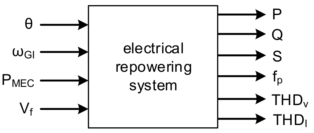
According to the IPS in Figure 8, the tests performed on a laboratory bench used a system composed of a synchronous generator $G_S$ and an induction generator $G_I$, connected in parallel [41]. The generators feed a nonlinear load $N_L$ (TPACVC) that consists of a three-phase rectifier that feeds a 14 kW resistive load. The primary machine used for $G_S$ was a diesel cycle engine with $38.7$ kW of power, and the primary machine used for $G_I$ was an induction motor with $7.5$ kW, driven by a frequency inverter with $9.2$ kW of power.

Table 1. Laboratory bench technical specifications. Adapted from [69].

Acronym	Component	Technical Specifications
$G_S$	synchronous generator	37 kVA, 380 V, $f_p$ $0.8$
		three-phase, salient
	(main generator)	4 poles, 60 Hz
$G_I$	induction generator	7.5 kVA, 380 V
		three-phase, cage rotor
		4 poles, 60 Hz
$T_L$	main feeder	three-phase, 13,800 V, 60 Hz
$T_1$	transformer	750 kVA, 13,800/(380/220) V
		$\Delta$/Y grounded
$N_L$	nonlinear load	14 kW three-phase, 380 V, 60 Hz

presents in detail the components technical specifications used in the laboratory bench.

The simulations performed with the IPS in Figure 8 used a model determined by parametric regression technique [69]. In the model designing process, a hybrid strategy was adopted, consisting of Nelder-Mead and Genetic Algorithm methods association. Using the computational model, it is possible to run simulations that would be unfeasible with the real system, allowing the elaboration of different prediction types. Furthermore, the system input parameters can use a wider variation ranges, enabling the improvement of sensitivity analysis process. However, in performed studies, the system input parameters values were changed within the range of feasible values, in order to eliminate conditions that could compromise its physical limit. As the system input parameters have different variation ranges and considering that some of them can vary only in the vicinity of their reference values, the analytical method [60] of sensitivity analysis is suitable for experiments involving this system.

4.1. Sensitivity Analysis and Parameters Suppression of Electrical Repowering System

The electrical repowering system sensitivity analysis was performed for both experimental tests and computational simulations results.

Table 2. Base values and variation ranges for electrical repowering system input parameters.

Parameter	Base Value	Laboratory Bench		Computer Simulated
		Variation Range	Variation	Variation Range	Variation
$\theta$	${132.83}^{\circ }$	(${80.85}^{\circ }$, ${140.5}^{\circ }$)	($-39.13\%$, $5.77\%$)	($2^{\circ }$, ${180}^{\circ }$)	($-98.49\%$, $35.51\%$)
${\omega }_{GI}$	1840 rpm	(1815 rpm, 1855 rpm)	($-1.36\%$, $0.81\%$)	(1800 rpm, 1860 rpm)	($-2.17\%$, $1.09\%$)
$P_{MEC}$	$18.87$ kVA	($11.21$ kVA, $18.87$ kVA)	($-40.59\%$, $0\%$)	($10.00$ kVA, $37.00$ kVA)	($-47.00\%$, $96.08\%$)
$V_f$	$41.5$ V	($38.8$ V, 48 V)	($-6.51\%$, $15.66\%$)	($28.92$ V, $71.77$ V)	($-30.31\%$, $74.70\%$)

[41] has base values of input parameters $\theta$, ${\omega }_{GI}$, $P_{MEC}$, and $V_f$ and their respective variation ranges within the feasible operating space of the system. The base values chosen are equivalent to median values relative to the lower and upper limits accepted by the laboratory bench. The variation range adopted for system input parameters values is greater in computer simulations than in experiments with the laboratory bench, allowing system analysis under a greater number of operating regimes.

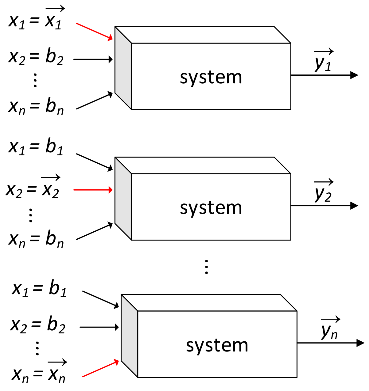
Experiments with the laboratory bench and computer simulations were carried out, varying the parameters in Table 2 one-at-a-time, considering their respective base values as reference and collecting outputs P, Q, S, $f_p$, $TH{D}_V$, and $TH{D}_I$. Using (1), the sensitivity indices were calculated for each system input parameter relative to each output.

Table 3. Sensitivity indices of electrical repowering system input parameters: laboratory bench and computer simulated.

Output	Laboratory Bench				Computer Simulated
	${\mathit{S}}_{\mathbf{\theta }}$	${\mathit{S}}_{{\mathbf{\omega }}_{\mathit{GI}}}$	${\mathit{S}}_{{\mathit{P}}_{\mathit{MEC}}}$	${\mathit{S}}_{{\mathit{V}}_{\mathit{f}}}$	${\mathit{S}}_{\mathbf{\theta }}$	${\mathit{S}}_{{\mathbf{\omega }}_{\mathit{GI}}}$	${\mathit{S}}_{{\mathit{P}}_{\mathit{MEC}}}$	${\mathit{S}}_{{\mathit{V}}_{\mathit{f}}}$
P	0.31	0.12	0.55	0.02	0.41	0.13	0.45	0.01
Q	0.06	0.02	0.64	0.28	0.06	0.01	0.56	0.37
S	0.18	0.09	0.60	0.13	0.19	0.08	0.61	0.12
$f_p$	0.24	0.06	0.40	0.30	0.36	0.05	0.32	0.27
$TH{D}_V$	0.48	0.23	0.15	0.14	0.21	0.10	0.59	0.10
$TH{D}_I$	0.22	0.04	0.61	0.13	0.48	0.07	0.34	0.11
average	0.25	0.09	0.49	0.17	0.29	0.07	0.48	0.16

[41] provides the results. For the sensitivity analysis process, each input parameter used 61 linearly spaced values considering their respective variation ranges. On average, both in experimental tests and simulations, of four analyzed parameters, $P_{MEC}$ is the one with highest sensitivity, followed by $\theta$, $V_f$, and ${\omega }_{GI}$.

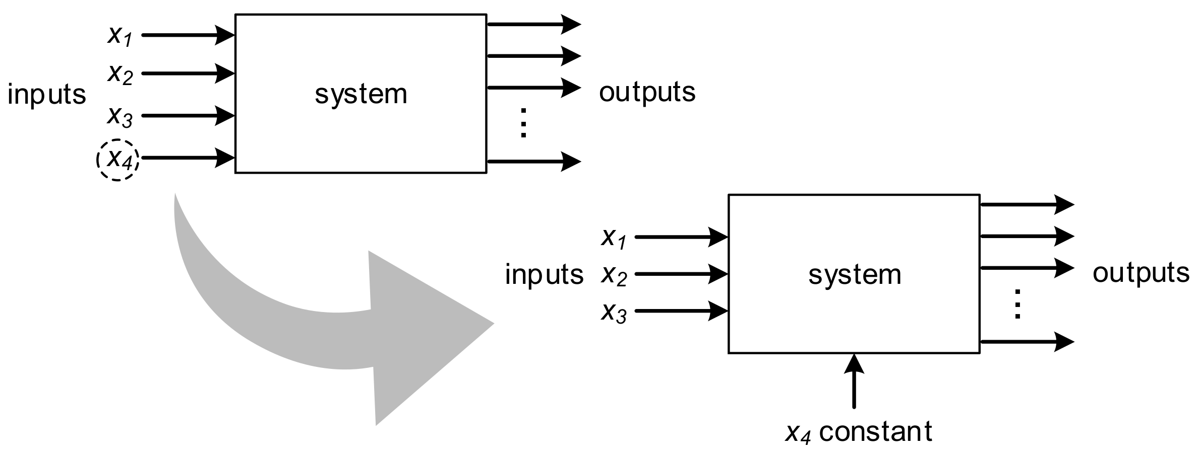
Considering the fact that the sensitivity index value of the parameter $V_f$ is the smallest for output P and the fact that the sensitivity index value of the parameter ${\omega }_{GI}$ is the smallest for Q, S, $f_p$, $TH{D}_V$, and $TH{D}_I$ outputs, we suppress these parameters according to the methodology presented in Section 3.1. Figure 10 represents the electrical repowering system with reduced quantity from four to three input parameters. Figure 10a,b represent the system with suppression of the parameters $V_f$ and ${\omega }_{GI}$, respectively. As the electrical repowering system is a nonlinear system, the suppression of some of its input parameters implies the modification of the remaining parameter’s sensitivity indices values. Thus, we performed two new sensitivity analysis processes: one considering the suppression of the $V_f$ parameter and the other considering the suppression of ${\omega }_{GI}$. These new analyses used base values and ranges, the results of which are displayed in Table 2 and

Table 4. Sensitivity indices values of input parameters considering both the original and one input parameter suppressed systems.

Output	Number of	${\mathit{S}}_{\mathbf{\theta }}$	${\mathit{S}}_{{\mathbf{\omega }}_{\mathit{GI}}}$	${\mathit{S}}_{{\mathit{P}}_{\mathit{MEC}}}$	${\mathit{S}}_{{\mathit{V}}_{\mathit{f}}}$
	Input Parameters
P	4	0.41	0.13	0.45	0.01
	3	0.32	0.12	0.56	–
Q	4	0.06	0.01	0.56	0.37
	3	0.06	–	0.56	0.38
S	4	0.19	0.08	0.61	0.12
	3	0.21	–	0.67	0.12
$f_p$	4	0.36	0.05	0.32	0.27
	3	0.38	–	0.34	0.28
$TH{D}_V$	4	0.21	0.10	0.59	0.10
	3	0.24	–	0.65	0.11
$TH{D}_I$	4	0.48	0.07	0.34	0.11
	3	0.52	–	0.37	0.11

.

Sensitivity indices for output P, relative to the analysis of the system with four and three inputs, considering the suppression of $V_f$, are given in Table 4. For Q, S, $f_p$, $TH{D}_V$ and $TH{D}_I$ outputs, Table 4 has the sensitivity indices relative to the analysis of the system with four and three entries, considering the suppression of ${\omega }_{GI}$.

Analyzing Table 4 for output P, considering the analysis with four variables, the sensitivity of parameter $\theta$ was 41% and that parameter $P_{MEC}$ was 45%. In the analysis considering three variables (suppressing $V_f$), the sensitivity of parameter $\theta$ was 32% and parameter $P_{MEC}$ was 56%. Therefore, comparing the analyses with four and three parameters, it is observed that the sensitivity of the parameter $\theta$ varied 22% and the sensitivity of the parameter $P_{MEC}$ varied 24%, confirming these parameters as the most sensitive relative to the output P. For Q output, when comparing the analyses with four and three parameters (suppressing parameter ${\omega }_{GI}$), parameters $P_{MEC}$ and $V_f$ were the ones with the highest sensitivity, with a reduced variation percentage between analyses.

According to Table 4, $\theta$ and $P_{MEC}$ were the parameters with the highest sensitivity relative to outputs S, $f_p$, $TH{D}_V$, and $TH{D}_I$, both in the analyses considering four parameters as for analyses considering three parameters and suppression of ${\omega }_{GI}$. Comparing analyses, the variation of parameters $\theta$ and $P_{MEC}$ was equal to 10%, considering output S. For $f_p$ output, the variation of parameters $\theta$ and $P_{MEC}$ was 5%. Variations of $\theta$ and $P_{MEC}$ were equal to 12% and 9%, respectively, for output $TH{D}_V$. For output $TH{D}_I$, the variation of both $\theta$ and $P_{MEC}$ was 8%, considering both analyses.

Still examining Table 4, it is possible to notice that the suppressed parameter sensitivity index value is distributed among other parameters, with a tendency of a higher increase in the most sensitive parameter index value. Therefore, suppressing the $V_f$ parameter in analyses involving the P output and suppressing the ${\omega }_{GI}$ parameter in analyses involving Q, S, $f_p$, $TH{D}_V$, and $TH{D}_I$ outputs do not harm the developed model accuracy for the electrical repowering system.

4.2. Electrical Repowering System Stability

In order to validate the proposed system stability metric, we applied it to the model developed for the electrical repowering system. To do so, we establish the sequence ${\delta }^S=({\delta }^1,{\delta }^2,{\delta }^3,{\delta }^4,{\delta }^5)$ with different operating scenarios, varying the input parameters values of the modeled system, as shown in

Table 5. Electrical repowering system input parameter values for different operating scenarios.

Scenario	Values for Input Parameters	Variation from Base Case	Description
	[$\mathit{\theta }$, ${\mathit{\omega }}_{\mathit{GI}}$, ${\mathit{P}}_{\mathit{MEC}}$, ${\mathit{V}}_{\mathit{f}}$]	[$\mathbf{\theta }$, ${\mathbf{\omega }}_{\mathbf{GI}}$, ${\mathit{P}}_{\mathit{MEC}}$, ${\mathit{V}}_{\mathit{f}}$]	Base Case Values Varied by…
${\delta }^1$	(${99.62}^{\circ }$, 1800 rpm, $14.15$ kVA, $31.1$ V)	(−25%, −2.22%, −25%, −25%)	… −25%, except ${\omega }_{GI}$
${\delta }^2$	(${119.55}^{\circ }$, 1822 rpm, $16.98$ kVA, $37.3$ V)	(−10%, −0.98%, −10%, −10%)	… −10%, except ${\omega }_{GI}$
${\delta }^3$	(${132.83}^{\circ }$, 1840 rpm, $18.87$ kVA, $41.5$ V)	(0%, 0%, 0%, 0%)	… 0%
${\delta }^4$	(${146.11}^{\circ }$, 1858 rpm, $20.75$ kVA, $45.6$ V)	(10%, 0.97%, 10%, 10%)	… 10%, except ${\omega }_{GI}$
${\delta }^5$	(${166.04}^{\circ }$, 1860 rpm, $23.58$ kVA, $47.2$ V)	(25%, 1.08%, 25%, 13.73%)	… 25%, except ${\omega }_{GI}$ and $V_f$

. The scenario ${\delta }^3$ refers to the base case, defined in the sensitivity analysis section (Section 4.1). Scenarios ${\delta }^1$, ${\delta }^2$, ${\delta }^4$ and ${\delta }^5$ varied the input parameters $\theta$ and $P_{MEC}$ values by $-25\%$, $-10\%$, $10\%$ and $25\%$, respectively, relative to base case. The value of input parameter ${\omega }_{GI}$ in scenarios ${\delta }^1$, ${\delta }^2$, ${\delta }^4$, and ${\delta }^5$ varied by $-2.22\%$, $-0.98\%$, $0.97\%$, and $1.08\%$, respectively, relative to the base case. The upper limit of 1860 rpm observed in ${\delta }^5$ arises from the limit rotation of the induction motor connected to $G_I$ and the lower limit of 1800 rpm in ${\delta }^1$ comes from the fact that below such speed, $G_I$ operates as a motor. The input parameter $V_f$ had its value varied by $-25\%$, $-10\%$, and $10\%$, relative to the base case, in scenarios ${\delta }^1$, ${\delta }^2$, and ${\delta }^4$, respectively. In ${\delta }^5$ the variation was $13.73\%$ relative to the base case. This variation is due to the fact that the limit value of $V_f$ for $G_S$ to operate as an inductive machine (i.e., receive reactive power from the network) is $47.2$ V.

Considering the input parameters values of Table 5, it is possible to establish the following assumptions: (i) harmonic distortion in the system increases as value of $\theta$ increases, (ii) as ${\omega }_{GI}$ and $P_{MEC}$ increase, the active power P also increases, and (iii) the increase of $V_f$ implies the increase in reactive power Q.

After performing the sensitivity analysis process considering each scenario in Table 5, we calculated the stability of each input parameter relative to the system outputs using (3). The values obtained for stabilities $\xi \left(\theta \right)$, $\xi \left({\omega }_{GI}\right)$, $\xi \left(P_{MEC}\right)$, and $\xi \left(V_f\right)$ relative to system outputs P, Q, S, $f_p$, $TH{D}_V$, and $TH{D}_I$ are arranged in

Table 6. Stability values of electrical repowering system input parameters relative to its outputs.

Scenario	Output	$\mathbf{\xi }\left(\mathbf{\theta }\right)$	$\mathbf{\xi }\left({\mathbf{\omega }}_{\mathit{GI}}\right)$	$\mathbf{\xi }\left({\mathit{P}}_{\mathit{MEC}}\right)$	$\mathbf{\xi }\left({\mathit{V}}_{\mathit{f}}\right)$
${\delta }^1$	P	0.7391	0.2145	0.8066	0.5861
	Q	0.7112	0.6326	0.9012	0.1424
	S	0.8072	0.2324	0.8760	0.4355
	$f_p$	0.7239	0.4141	0.9134	0.3746
	$TH{D}_V$	0.9672	0.9833	0.9672	0.9672
	$TH{D}_I$	0.6156	0.4262	0.6066	0.3306
	average	0.7607	0.4838	0.8452	0.4727
${\delta }^2$	P	0.7416	0.2158	0.6917	0.6063
	Q	0.7136	0.3440	0.9081	0.1573
	S	0.8041	0.1563	0.8796	0.5517
	$f_p$	0.7512	0.4025	0.9288	0.3574
	$TH{D}_V$	0.9672	0.9667	0.9672	0.9672
	$TH{D}_I$	0.6239	0.1383	0.6540	0.3634
	average	0.7669	0.3706	0.8382	0.5005
${\delta }^3$	P	0.7400	0.1206	0.5935	0.6358
	Q	0.7114	0.3640	0.8610	0.2796
	S	0.7989	0.1408	0.8112	0.6323
	$f_p$	0.7799	0.3683	0.8745	0.4660
	$TH{D}_V$	0.9672	0.9667	0.9672	0.9672
	$TH{D}_I$	0.6234	0.1329	0.6120	0.4634
	average	0.7701	0.3489	0.7866	0.5740
${\delta }^4$	P	0.7408	0.0733	0.4570	0.6997
	Q	0.7117	0.4825	0.8147	0.3246
	S	0.7959	0.0963	0.7236	0.6548
	$f_p$	0.7948	0.4452	0.8377	0.5124
	$TH{D}_V$	0.9672	0.9667	0.9672	0.9672
	$TH{D}_I$	0.6218	0.1436	0.5570	0.5079
	average	0.7720	0.3679	0.7262	0.6111
${\delta }^5$	P	0.7399	0.0673	0.3995	0.7264
	Q	0.7107	0.5223	0.8039	0.4027
	S	0.7987	0.0994	0.6875	0.6698
	$f_p$	0.7892	0.8545	0.8360	0.5578
	$TH{D}_V$	0.9672	0.9833	0.9672	0.9672
	$TH{D}_I$	0.6212	0.1137	0.5235	0.5732
	average	0.7712	0.4401	0.7029	0.6495

.

Based on Table 6, it is possible to observe that in scenarios ${\delta }^1$ and ${\delta }^2$, considering the average row, the input parameters $P_{MEC}$ and $\theta$ are the most stable relative to system outputs, followed by $V_f$ and ${\omega }_{GI}$. In ${\delta }^3$ and ${\delta }^4$ scenarios: (i) parameters $\theta$ and $V_f$ are the most stable relative to system output P, followed by $P_{MEC}$ and ${\omega }_{GI}$, and (ii) parameters $P_{MEC}$ and $\theta$ are the most stable relative to the other system outputs, followed by $V_f$ and ${\omega }_{GI}$. In ${\delta }^5$ scenario: (i) parameters $\theta$ and $V_f$ are the most stable relative to outputs P and $TH{D}_I$, followed by $P_{MEC}$ and ${\omega }_{GI}$, (ii) relative to outputs Q and S, parameters $P_{MEC}$ and $\theta$ are the most stable, followed by $V_f$ and ${\omega }_{GI}$, (iii) considering output $f_p$, parameters ${\omega }_{GI}$ and $P_{MEC}$ are the most stable, followed by $\theta$ and $V_f$, and (iv) for output $TH{D}_V$, parameter ${\omega }_{GI}$ is the most stable, followed by parameters $\theta$, $P_{MEC}$, and $V_f$.

Considering the average row of all scenarios arranged in Table 6, it is possible to see: (i) $\theta$ and $P_{MEC}$ are the most stable input parameters, followed by parameters $V_f$ and ${\omega }_{GI}$, (ii) the $\theta$ parameter stability remains practically constant, (iii) there is a small reduction in stability of parameter $P_{MEC}$, (iv) there is a slight increase in stability of parameter $V_f$, and (v) parameter ${\omega }_{GI}$ has greater stability in scenarios with greater variation (i.e., ${\delta }^1$ and ${\delta }^5$) compared with the base scenario.

Comparing stability values of $\theta$ relative to $TH{D}_I$, and then with each scenario average rows in Table 6, we observe a constant variation of approximately 81%. Even increasing $\theta$, this parameter’s stability relative to $TH{D}_I$ remains stable.

Analyzing Table 6, it is possible to see that stability values of ${\omega }_{GI}$ and $P_{MEC}$ relative to P decrease in each scenario, being smaller than their respective values in the average rows. Considering these analyses and Table 1, we can affirm that the powers of $G_S$ and $G_I$ machines influence stability. The power of $G_S$ is five times greater than the power of $G_I$, which implies that $P_{MEC}$ impacts the active power flow P more than ${\omega }_{GI}$.

Comparing the stability values of $V_f$ relative to Q, and then with each scenario average row in Table 6, it is possible to observe variations of 30.12%, 31.42%, 48.71%, 53.11% and 62%. This increasing percentage of variation confirms the relationship between parameter $V_f$ and output Q, since as $V_f$ increases, its stability relative to Q also increases.

Table 7. Differences between minimum and maximum stability values of electrical repowering system parameters relative to its outputs.

Output	${\mathbf{\xi }}_{\mathit{max}}-{\mathbf{\xi }}_{\mathit{min}}$
	$\mathbf{\theta }$	${\mathbf{\omega }}_{\mathit{GI}}$	${\mathit{P}}_{\mathit{MEC}}$	${\mathit{V}}_{\mathit{f}}$
P	0.0025	0.1485	0.4071	0.1403
Q	0.0029	0.2886	0.1042	0.2603
S	0.0113	0.1330	0.1921	0.2343
$f_p$	0.0709	0.4862	0.0928	0.2004
$TH{D}_V$	0.0000	0.0166	0.0000	0.0000
$TH{D}_I$	0.0083	0.3125	0.1305	0.2426

displays the differences between maximum and minimum stability value, ${\xi }_{max}-{\xi }_{min}$, of each parameter relative to the system outputs, considering each scenario from Table 6. For example, as the greatest stability value of $\theta$ relative to output P is $0.7416$ and the smallest value is $0.7391$, the difference between these values ($0.0025$) is in the first row and first column of Table 7. The $\theta$ input parameter showed the smallest difference between maximum and minimum stability values relative to all outputs. This fact confirms this parameter’s high stability, even when the electrical repowering system operates in different studied scenarios.

The observed difference between maximum and minimum stability values of all input parameters relative to $TH{D}_V$ in Table 7 was equal to $zero$, except for ${\omega }_{GI}$ (with a value of ≈$zero$). In parallel, the difference between the maximum and minimum stability values of ${\omega }_{GI}$ relative to $TH{D}_I$ was the third-largest recorded, being higher than the other differences observed for this output. These facts indicate the induction generator $G_I$ capacity to absorb harmonic distortions, which confirms the results of Magalhães et al. [41].

Considering scenario ${\delta }^3$ and suppressing ${\omega }_{GI}$ (Section 3.1), we performed a new stability analysis.

Table 8. Stability values of electrical repowering system input parameters relative to its outputs considering the scenario ${\delta }^3$ and suppressing parameter ${\omega }_{GI}$.

Analysis Characteristics	Output	$\mathbf{\xi }\left(\mathbf{\theta }\right)$	$\mathbf{\xi }\left({\mathbf{\omega }}_{\mathit{GI}}\right)$	$\mathbf{\xi }\left({\mathit{P}}_{\mathit{MEC}}\right)$	$\mathbf{\xi }\left({\mathit{V}}_{\mathit{f}}\right)$
suppressed ${\omega }_{GI}$ in ${\delta }^3$ scenario	P	0.7400	-	0.5935	0.6358
	Q	0.7114	-	0.8610	0.2796
	S	0.7989	-	0.8112	0.6323
	$f_p$	0.7799	-	0.8745	0.4660
	$TH{D}_V$	0.9672	-	0.9672	0.9672
	$TH{D}_I$	0.6234	-	0.6120	0.4634
	average	0.7701	-	0.7866	0.5740

displays the obtained values for $\theta$, $P_{MEC}$, and $V_f$ stabilities relative to outputs P, Q, S, $f_p$, $TH{D}_V$, and $TH{D}_I$. We observe that stability values obtained after the parameter suppression are the same as in scenario ${\delta }^3$ of Table 6, if we disregard the column referring to ${\omega }_{GI}$. Therefore, the stability of the electrical repowering system does not change when considering the input parameter ${\omega }_{GI}$ constant.

5. Discussion

The sensitivity analysis process, performed by varying the system’s input parameters and measuring its outputs, allows the construction of the spider diagram. Considering the angles formed between the line segments that make up each curve in the diagram and horizontal axis, we stipulate a stability metric. However, the system’s operating limits determine the minimum and maximum values for its parameter values, which limits the variation ranges used in the sensitivity analysis. This limitation can be observed in electrical repowering system analysis, in which the parameter variation interval ${\omega }_{GI}$ was significantly smaller than the variation interval of other parameters (93.4% smaller than $\theta$ and $P_{MEC}$ variation interval and 91.5% smaller than $V_f$ variation). For the sensitivity analysis of systems with this characteristic, one of the recommended methods is the analytical method proposed by Gomes et al. [60]. However, the proposed methodology in Figure 7 is not limited to the use of this method; thus, other sensitivity analysis methods such as the area method, partial derivatives, factorial planning, conditional variance, and the total effects method [70,71,72,73] can be used.

To perform the stability study of systems with multiple outputs, it is necessary to execute a sensitivity analysis of their input parameters considering each of their outputs. Thus, for a system with n parameters and $n_{out}$ outputs, $n\times n_{out}$ stability values must be calculated. When suppressing a system parameter, this quantity is reduced to $(n-1)\times n_{out}$ and so on. To ensure the assertiveness of analyses performed with the reduced system, it is necessary to certify that suppressing the chosen parameter does not affect its response in terms of sensitivity and stability. To check this match, a new sequence of analyses is required.

In the electrical repowering system stability study, we performed the suppression of the system’s least sensitive parameter: ${\omega }_{GI}$. We found that suppressing this parameter did not affect the stability values of other system parameters. This fact suggests that analyses involving the sensitivity and stability of the modeled electrical repowering system can be performed considering fixed ${\omega }_{GI}$.

Since the stability values are in the closed interval $[0,1]$, it is possible to determine, depending on the analysis interest, subintervals that represent the different stability levels of the system. In this way, is possible to group parameters $\theta$, ${\omega }_{GI}$, $P_{MEC}$, and $V_f$ into different categories, according to their stability relative to the system outputs. A possible sequence of stability subintervals for arbitrary parameter $x_i$ can be determined by: (i) $0\le \xi \left(x_i\right)\le 0.6$, representing low stability, (ii) $0.6<\xi \left(x_i\right)\le 0.8$, representing moderate stability, and (iii) $0.8<\xi \left(x_i\right)\le 1$, representing high stability. Considering these subintervals and the values related to scenario ${\delta }^3$ in Table 6, it is possible to say, for example, that parameter ${\omega }_{GI}$ has low stability relative to output P, parameter $\theta$ presents moderate stability relative to output $f_p$ and parameter $P_{MEC}$ presents high stability relative to output Q. Figure 11 shows the number of occurrences of each stability category in Table 6 scenarios.

Looking at Figure 11, it is possible to note: (i) greater predominance of values belonging to the low stability category, (ii) equal occurrence count of each category in scenarios ${\delta }^3$ and ${\delta }^5$, and (iii) different order in number of occurrences of each category in scenario ${\delta }^2$. The notion of stability categories enables the creation of mechanisms to classify system operation scenarios. This classification can be performed, for example, by assigning weights to each stability category determined for the system, followed by the calculation of a single stability index for the scenario.

In large-scale power systems with several buses, a problem emerges regarding the number of electrical measuring points. For systems with thousands of elements, it is challenging to record data from the entire system. Figure 12 illustrates a power system with a synchronous generator connected in parallel with an induction generator. These machines feed numerous loads represented by b-buses. To use the proposed stability metric in such systems, it is recommended to perform power measurements at representative points depending on the accuracy of analysis (e.g., buses 1, $b/2$, and b). Additionally, values recorded from the power measurements must be compared with the ones obtained from power flow simulations to ensure accurate sensitivity and stability analyses.

When using the proposed metric for large-scale systems such as the one exhibited in Figure 12, the computational time required for calculating system stability can be measured by identifying the time spent ($t_s$) to compute a single stability value relative to one output. The $t_s$ is hardware-dependent, i.e., it depends on the processing power provided by the machine used to execute the simulations. To obtain the total time spent to perform the system stability analysis, $t_s\times (n\times n_{out})$ must be calculated. In addition to computational time spent in system stability analysis, the time spent to obtain the data used in the analysis must be considered. However, automated data collection mechanisms can be implemented in the system, significantly reducing this time.

Using the proposed methodologies, it is possible to conduct studies involving a wide range of engineering systems. These studies may contain analyses regarding the system’s stability, considering its original form or its form reducing one or more input parameters. We suggest the following system categories for stability studies: production and logistics chains, electrical and electronic systems, healthcare systems, and computerized information systems.

6. Conclusions

In this paper, we propose a system stability metric. To quantify stability, we measure the oscillation level of the system output, measuring the impact of disturbances and external influences through sensitivity analysis. System stability analysis enables: (i) determining feasible limits for its input parameters variation, without compromising its regular operation, (ii) improving its project, as it allows behavior prediction under adverse operating situations, such as idleness and overload, (iii) preventing cascading failures, given the networked nature of current systems, and (iv) its study from an input/output relationship perspective. As the proposed stability metric considers the Systems Science background, it can be applied to systems that allow variation in the values of their input parameters and verification of the impact of these variations on their outputs. We apply the proposed stability metric to an electrical repowering system and analyze the stability values of its inputs relative to its outputs. As a further investigation, we apply the parameter suppression process to this system. We compare the stability analysis results of the original system with analysis results of the system with reduced input parameters. We found that, in addition to the mentioned advantages, the stability study associated with the input parameter suppression technique allows for a smaller number of simulations in the system analysis process. Requiring less computational effort to perform experiments with reduced systems as a practical implication. Associating the proposed stability metric with other system metrics found in the literature, such as performance, complexity, and robustness, allows multifaceted analysis and/or elaboration of optimization strategies.

References

1. Kundur, P. Power System Stability and Control, 1st ed.; McGraw-Hill Education: New York, NY, USA, 1994. [Google Scholar]
2. Klir, G.J. Facets of Systems Science; Springer: New York, NY, USA, 2013; Volume 7. [Google Scholar]
3. Mobus, G.E.; Kalton, M.C. Principles of Systems Science, 1st ed.; Springer: New York, NY, USA, 2015. [Google Scholar]
4. Jen, E. Robust Design: A Repertoire of Biological, Ecological, and Engineering Case Studies; Oxford University Press: Oxford, UK, 2005. [Google Scholar]
5. Xue, A.; Mei, S.; Xie, B. A comprehensive method to compute the controlling unstable equilibrium point. In Proceedings of the 2008 Third International Conference on Electric Utility Deregulation and Restructuring and Power Technologies, Nanjing, China, 6–9 April 2008; pp. 1115–1120. [Google Scholar] [CrossRef]
6. Qiaoge, L.; Mengyin, F.; Changsheng, S. Study of the control-equilibrium of control systems. J. Syst. Eng. Electron. 2008, 19, 775–778. [Google Scholar] [CrossRef]
7. Avramov, K.; Mikhlin, Y.V. Forced oscillations of a system, containing a snap-through truss, close to its equilibrium position. Nonlinear Dyn. 2004, 35, 361–379. [Google Scholar] [CrossRef]
8. Serway, R.A.; Jewett, J.W. Principles of Physics: A Calculus-Based Text; Cengage Learning: Harrisonburg, VA, USA, 2012; Volume 2. [Google Scholar]
9. Paice, A.; Wirth, F. Analysis of the local robustness of stability for maps. In Proceedings of the 1997 European Control Conference (ECC), Brussels, Belgium, 1–7 July 1997; pp. 1259–1264. [Google Scholar] [CrossRef]
10. Thomas, D.G.; Bywaters, D.S. System Stability and Conclusions. In The Creators of Inside Money; Springer: New York, NY, USA, 2021; pp. 211–215. [Google Scholar] [CrossRef]
11. Bai, L.; Zhou, W. The measurement of transient stability with high resolution. In Proceedings of the 2013 Joint European Frequency and Time Forum & International Frequency Control Symposium (EFTF/IFC), Prague, Czech Republic, 21–25 July 2013; pp. 175–178. [Google Scholar] [CrossRef]
12. Chestnov, V.; Shatov, D. Modified circle criterion of absolute stability and robustness estimation. In Proceedings of the 2018 14th International Conference Stability and Oscillations of Nonlinear Control Systems (Pyatnitskiy’s Conference) (STAB), Moscow, Russia, 30 May–1 June 2018; pp. 1–4. [Google Scholar] [CrossRef]
13. Pesterev, A. Absolute stability analysis for a linear time varying system of special form. In Proceedings of the 2016 International Conference Stability and Oscillations of Nonlinear Control Systems (Pyatnitskiy’s Conference), Moscow, Russia, 1–3 June 2016; pp. 1–3. [Google Scholar] [CrossRef]
14. Wolf, A.; Swift, J.B.; Swinney, H.L.; Vastano, J.A. Determining Lyapunov exponents from a time series. Phys. D Nonlinear Phenom. 1985, 16, 285–317. [Google Scholar] [CrossRef] [Green Version]
15. Okuyama, Y. Stability analysis of discrete event systems using multiple metrics and simultaneous linear inequalities. In Proceedings of the 2016 55th Annual Conference of the Society of Instrument and Control Engineers of Japan (SICE), Tsukuba, Japan, 20–23 September 2016; pp. 1141–1146. [Google Scholar] [CrossRef]
16. Liu, Z.; He, X.; Ding, Z.; Zhang, Z. A Basin Stability Based Metric for Ranking the Transient Stability of Generators. IEEE Trans. Ind. Inform. 2019, 15, 1450–1459. [Google Scholar] [CrossRef]
17. White, K.L.; Chaubey, I. Sensitivity analysis, calibration, and validations for a multisite and multivariable SWAT model 1. JAWRA J. Am. Water Resour. Assoc. 2005, 41, 1077–1089. [Google Scholar] [CrossRef]
18. Kamiński, B.; Jakubczyk, M.; Szufel, P. A framework for sensitivity analysis of decision trees. Cent. Eur. J. Oper. Res. 2018, 26, 135–159. [Google Scholar] [CrossRef]
19. Hamby, D.M. A review of techniques for parameter sensitivity analysis of environmental models. Environ. Monit. Assess. 1994, 32, 135–154. [Google Scholar] [CrossRef]
20. Frey, H.C.; Patil, S.R. Identification and review of sensitivity analysis methods. Risk Anal. 2002, 22, 553–578. [Google Scholar] [CrossRef]
21. Saltelli, A.; Tarantola, S.; Campolongo, F.; Ratto, M. Sensitivity Analysis in Practice: A Guide to Assessing Scientific Models; Wiley Online Library: Hoboken, NJ, USA, 2004; Volume 1. [Google Scholar]
22. Borgonovo, E.; Plischke, E. Sensitivity analysis: A review of recent advances. Eur. J. Oper. Res. 2016, 248, 869–887. [Google Scholar] [CrossRef]
23. Qian, G.; Mahdi, A. Sensitivity analysis methods in the biomedical sciences. Math. Biosci. 2020, 323, 108306. [Google Scholar] [CrossRef]
24. Razavi, S.; Jakeman, A.; Saltelli, A.; Prieur, C.; Iooss, B.; Borgonovo, E.; Plischke, E.; Piano, S.L.; Iwanaga, T.; Becker, W.; et al. The future of sensitivity analysis: An essential discipline for systems modeling and policy support. Environ. Model. Softw. 2021, 137, 104954. [Google Scholar] [CrossRef]
25. Triantaphyllou, E.; Sánchez, A. A sensitivity analysis approach for some deterministic multi-criteria decision-making methods. Decis. Sci. 1997, 28, 151–194. [Google Scholar] [CrossRef]
26. Pannell, D.J. Sensitivity analysis: Strategies, methods, concepts, examples. Agric. Econ. 1997, 16, 139–152. [Google Scholar] [CrossRef]
27. Kumar, R.; Dubey, R.; Singh, S.; Singh, S.; Prakash, C.; Nirsanametla, Y.; Królczyk, G.; Chudy, R. Multiple-Criteria Decision-Making and Sensitivity Analysis for Selection of Materials for Knee Implant Femoral Component. Materials 2021, 14, 2084. [Google Scholar] [CrossRef] [PubMed]
28. Saraiva, J.P.; Lima, B.S.; Gomes, V.M.; Flores, P.H.; Gomes, F.A.; Assis, A.O.; Reis, M.R.; Araújo, W.R.; Abrenhosa, C.; Calixto, W.P. Calculation of sensitivity index using one-at-a-time measures based on graphical analysis. In Proceedings of the 2017 18th International Scientific Conference on Electric Power Engineering (EPE), Kouty nad Desnou, Czech Republic, 17–19 May 2017; pp. 1–6. [Google Scholar] [CrossRef]
29. Pianosi, F.; Wagener, T. Distribution-based sensitivity analysis from a generic input-output sample. Environ. Model. Softw. 2018, 108, 197–207. [Google Scholar] [CrossRef] [Green Version]
30. Kim, N.H.; Wang, H.; Queipo, N.V. Adaptive reduction of random variables using global sensitivity in reliability-based optimisation. Int. J. Reliab. Saf. 2006, 1, 102–119. [Google Scholar] [CrossRef] [Green Version]
31. Singh, S.S.; Fernandez, E. Modeling, size optimization and sensitivity analysis of a remote hybrid renewable energy system. Energy 2018, 143, 719–731. [Google Scholar] [CrossRef]
32. Zhu, X.; Huang, J.; Quan, L.; Xiang, Z.; Shi, B. Comprehensive sensitivity analysis and multiobjective optimization research of permanent magnet flux-intensifying motors. IEEE Trans. Ind. Electron. 2018, 66, 2613–2627. [Google Scholar] [CrossRef]
33. Hemeida, A.M.; Omer, A.S.; Bahaa-Eldin, A.M.; Alkhalaf, S.; Ahmed, M.; Senjyu, T.; El-Saady, G. Multi-objective multi-verse optimization of renewable energy sources-based micro-grid system: Real case. Ain Shams Eng. J. 2021. [Google Scholar] [CrossRef]
34. Helton, J.C.; Johnson, J.D.; Sallaberry, C.J.; Storlie, C.B. Survey of sampling-based methods for uncertainty and sensitivity analysis. Reliab. Eng. Syst. Saf. 2006, 91, 1175–1209. [Google Scholar] [CrossRef] [Green Version]
35. Mavromatidis, G.; Orehounig, K.; Carmeliet, J. Uncertainty and global sensitivity analysis for the optimal design of distributed energy systems. Appl. Energy 2018, 214, 219–238. [Google Scholar] [CrossRef]
36. vom Lehn, F.; Cai, L.; Pitsch, H. Sensitivity analysis, uncertainty quantification, and optimization for thermochemical properties in chemical kinetic combustion models. Proc. Combust. Inst. 2019, 37, 771–779. [Google Scholar] [CrossRef]
37. Sols, A. Validation of the robustness of the selection of the preferred design concept through a comprehensive sensitivity analysis. In Proceedings of the Systems Conference (SysCon), 2015 9th Annual IEEE International, Vancouver, BC, Canada, 13–16 April 2015; pp. 403–408. [Google Scholar] [CrossRef]
38. Dosi, G.; Pereira, M.C.; Virgillito, M.E. On the robustness of the fat-tailed distribution of firm growth rates: A global sensitivity analysis. J. Econ. Interact. Coord. 2018, 13, 173–193. [Google Scholar] [CrossRef] [Green Version]
39. Syriopoulou, E.; Mozumder, S.I.; Rutherford, M.J.; Lambert, P.C. Robustness of individual and marginal model-based estimates: A sensitivity analysis of flexible parametric models. Cancer Epidemiol. 2019, 58, 17–24. [Google Scholar] [CrossRef] [PubMed]
40. Dao, D.V.; Adeli, H.; Ly, H.B.; Le, L.M.; Le, V.M.; Le, T.T.; Pham, B.T. A sensitivity and robustness analysis of GPR and ANN for high-performance concrete compressive strength prediction using a Monte Carlo simulation. Sustainability 2020, 12, 830. [Google Scholar] [CrossRef] [Green Version]
41. Magalhaes, A.S.; Bulhoes, J.S.; Reis, M.R.; Gomes, V.M.; Silva, A.H.; Alves, A.J.; Wainer, G.A.; Ganzaroli, C.A.; Araujo, W.R.; Calixto, W.P. Experimental study of induction generator as a repowering solution. Int. Trans. Electr. Energy Syst. 2020, 30, e12365. [Google Scholar] [CrossRef]
42. Hnydiuk-Stefan, A. Dual-Fuel Gas-Steam Power Block Analysis: Methodology and Continuous-Time Mathematical Models; Springer: New York, NY, USA, 2018. [Google Scholar]
43. Neto, L.; Cardoso, J.; Santos, S.; Delbone, E. Repowering and evaluation of new power of synchronous generators. In Proceedings of the 2009 IEEE International Electric Machines and Drives Conference, Miami, FL, USA, 3–6 May 2009; pp. 1058–1064. [Google Scholar] [CrossRef]
44. Reynolds, G. Repowering: Enhance what is there [steam power plants]. IEEE Power Eng. Rev. 2001, 21, 16–18. [Google Scholar] [CrossRef]
45. Gagliano, A.; Tina, G.; Nocera, F.; Patania, F. Technical and economic perspective for repowering of micro hydro power plants: A case study of an early XX century power plant. Energy Procedia 2014, 62, 512–521. [Google Scholar] [CrossRef] [Green Version]
46. Pham, K.D. Cogeneration application: Interconnection of induction generators with public electric utility. In Proceedings of the 1991 Rural Electric Power Conference. Papers presented at the 35th Annual Conference, Dearborn, MI, USA, 28–30 April 1991. [Google Scholar] [CrossRef]
47. Silva, V.Z.; Rezek, A.J.J.; Ogoulola, C.E.G. Alternatives to control the frequency increase in an electric system with synchronous and induction generators in parallel operation mode. Electr. Power Syst. Res. 2020, 180, 106136. [Google Scholar] [CrossRef]
48. Xu, L.; Cheng, M.; Wei, X.; Yan, X.; Zeng, Y. Dual Synchronous Rotating Frame Current Control of Brushless Doubly Fed Induction Generator Under Unbalanced Network. IEEE Trans. Power Electron. 2020, 36, 6712–6724. [Google Scholar] [CrossRef]
49. Vanço, W.E.; Silva, F.B.; de Oliveira, J.M.; Almeida Monteiro, J.R. Effects of harmonic pollution on salient pole synchronous generators and on induction generators operating in parallel in isolated systems. Int. Trans. Electr. Energy Syst. 2020, 30, e12359. [Google Scholar] [CrossRef]
50. Escosa, J.M.; Romeo, L.M. Optimizing CO2 avoided cost by means of repowering. Appl. Energy 2009, 86, 2351–2358. [Google Scholar] [CrossRef]
51. Magalhães, A.S.; Bulhões, J.S.; Matias, C.A.; Silva, A.H.; Furriel, G.P.; Reis, M.R.; Wainer, G.A.; Gomes, V.M.; Calixto, W.P.; Alves, A.J. Sensitivity analysis of the synchronous generation repowering system in parallel with induction generator. In Proceedings of the 2017 CHILEAN Conference on Electrical, Electronics Engineering, Information and Communication Technologies (CHILECON), Pucon, Chile, 18–20 October 2017; pp. 1–5. [Google Scholar] [CrossRef]
52. Bertalanffy, L.V. General System Theory: Foundations, Development, Applications; Braziller: New York, NY, USA, 1968. [Google Scholar]
53. Maier, M.W. Architecting Principles for Systems-of-Systems; INCOSE International Symposium; Wiley Online Library: Hoboken, NJ, USA, 1996; Volume 6, pp. 565–573. [Google Scholar] [CrossRef]
54. Rechtin, E.; Maier, M.W. The Art of Systems Architecting; CRC Press: Boca Raton, FL, USA, 2010. [Google Scholar]
55. Cassandras, C.G.; Lafortune, S. Introduction to Discrete Event Systems, 2nd ed.; Springer: New York, NY, USA, 2009. [Google Scholar]
56. Wainer, G.A. Discrete-Event Modeling and Simulation: A Practitioner’s Approach, 1st ed.; CRC Press: Chichester, UK, 2009. [Google Scholar]
57. Critchfield, G.C.; Willard, K.E.; Connelly, D.P. Probabilistic sensitivity analysis methods for general decision models. Comput. Biomed. Res. 1986, 19, 254–265. [Google Scholar] [CrossRef]
58. Homma, T.; Saltelli, A. Importance measures in global sensitivity analysis of nonlinear models. Reliab. Eng. Syst. Saf. 1996, 52, 1–17. [Google Scholar] [CrossRef]
59. Salas, E.A.L.; Henebry, G.M. A new approach for the analysis of hyperspectral data: Theory and sensitivity analysis of the Moment Distance Method. Remote Sens. 2014, 6, 20–41. [Google Scholar] [CrossRef] [Green Version]
60. Gomes, V.M.; Assis, A.O.; Matias, C.A.; Saraiva, J.P.; Gomes, F.A.; Wainer, G.A.; Lima, B.S.; Magalhães, A.S.; Calixto, W.P.; Flores, P.H.; et al. Analytical method for calculating the sensitivity index of system parameters. In Proceedings of the 2017 CHILEAN Conference on Electrical, Electronics Engineering, Information and Communication Technologies (CHILECON), Pucon, Chile, 18–20 October 2017; pp. 1–6. [Google Scholar] [CrossRef]
61. Chapman, S. Electric Machinery Fundamentals, 5th ed.; McGraw-Hill Science: New York, NY, USA, 2011. [Google Scholar]
62. Santoso, S.; McGranaghan, M.F.; Dugan, R.C.; Beaty, H.W. Electrical Power Systems Quality, 3rd ed.; McGraw-Hill Education: New York, NY, USA, 2012. [Google Scholar]
63. Eschenbach, T.G.; McKeague, L.S. Exposition on using graphs for sensitivity analysis. Eng. Econ. 1989, 34, 315–333. [Google Scholar] [CrossRef]
64. Burger, W.; Burge, M.J. Principles of Digital Image Processing: Fundamental Techniques; Springer: New York, NY, USA, 2010. [Google Scholar]
65. De Dinechin, F.; Istoan, M. Hardware implementations of fixed-point Atan2. In Proceedings of the 2015 IEEE 22nd Symposium on Computer Arithmetic, Lyon, France, 22–24 June 2015; pp. 34–41. [Google Scholar] [CrossRef] [Green Version]
66. Torres, V.; Valls, J.; Lyons, R. Fast-and low-complexity atan2 (a, b) approximation [tips and tricks]. IEEE Signal Process. Mag. 2017, 34, 164–169. [Google Scholar] [CrossRef]
67. Zhang, T.; Stackhouse, P.W., Jr.; Macpherson, B.; Mikovitz, J.C. A solar azimuth formula that renders circumstantial treatment unnecessary without compromising mathematical rigor: Mathematical setup, application and extension of a formula based on the subsolar point and atan2 function. Renew. Energy 2021, 172, 1333–1340. [Google Scholar] [CrossRef]
68. Rashid, M.H. Power Electronics: Circuits, Devices, and Applications; Pearson Education India: Bengaluru, India, 2009. [Google Scholar]
69. Silva, A.H.; Magalhaes, A.S.; Bulhoes, J.S.; Wainer, G.A.; Furriel, G.P.; Calixto, W.P. Parametric Regression Applied for Determination of Electrical Parameters of Synchronous and Induction Generators Operating in Parallel on the Electrical Energy Repowering System. Energies 2021, 14, 3875. [Google Scholar] [CrossRef]
70. Law, A.M.; Kelton, W.D.; Kelton, W.D. Simulation Modeling and Analysis; McGraw-Hill: New York, NY, USA, 2000; Volume 3. [Google Scholar]
71. Saltelli, A.; Ratto, M.; Andres, T.; Campolongo, F.; Cariboni, J.; Gatelli, D.; Saisana, M.; Tarantola, S. Global Sensitivity Analysis: The Primer; John Wiley & Sons: Hoboken, NJ, USA, 2008. [Google Scholar]
72. Sarrazin, F.; Pianosi, F.; Wagener, T. Global Sensitivity Analysis of environmental models: Convergence and validation. Environ. Model. Softw. 2016, 79, 135–152. [Google Scholar] [CrossRef] [Green Version]
73. Gomes, V.M.; Paiva, J.R.; Reis, M.R.; Wainer, G.A.; Calixto, W.P. Mechanism for Measuring System Complexity Applying Sensitivity Analysis. Complexity 2019, 2019, 1303241. [Google Scholar] [CrossRef]
Figure 1. Local sensitivity analysis for a system with multiple inputs and one output. One-at-a-time measurements are performed for each input system parameter.
Energies 14 07824 g001
Figure 2. Parameter suppression process in a system with four inputs and multiple outputs.
Energies 14 07824 g002
Figure 3. Keeping outputs y 1 , y 2 and y 3 considering the reduction from four to three input parameters.
Energies 14 07824 g003
Figure 4. Spider diagram for a hypothetical system with three input parameters.
Energies 14 07824 g004
Figure 5. Delimitation of right triangle with angle α , considering a specific line segment and the horizontal plane.
Energies 14 07824 g005
Figure 6. Cases of greater and less stability. (a) Greater stability: α = 0 . (b) Less stability: α = 90 .
Energies 14 07824 g006
Figure 7. Activity flowchart to obtain the x i parameter stability relative to the system output.
Energies 14 07824 g007
Figure 8. Interconnected Power System (IPS) used for case study. Adapted from [69].
Energies 14 07824 g008
Figure 9. Representation of inputs and outputs considered in the electrical repowering system study.
Energies 14 07824 g009
Figure 10. Electrical repowering system with reduced quantity from four to three input parameters. (a) V f suppression. (b) ω G I suppression.
Energies 14 07824 g010
Figure 11. Number of occurrences of each stability category in the selected electrical repowering system scenarios.
Energies 14 07824 g011
Figure 12. Single-line diagram of a power system with b-buses.
Energies 14 07824 g012