Machine-Learning-Based Carbon Footprint Management in the Frozen Vegetable Processing Industry

Abstract

In the paper, we present a method of automatic evaluation and optimization of production processes towards low-carbon-emissions products. The method supports the management of production lines and is based on unsupervised machine learning methods, i.e., canopy, k-means, and expectation-maximization clusterization algorithms. For different production processes, a different clustering method may be optimal. Hence, they are validated by classification methods (k-nearest neighbors (kNN), multilayer perceptron (MLP), binary tree C4.5, random forest (RF), and support vector machine (SVM)) that identify the optimal clusterization method. Using the proposed method with real-time production parameters for a given process, we can classify the process as optimal or non-optimal on an ongoing basis. The production manager can react appropriately to sub-optimal production processes. If the process is not optimal, then during the process the manager or production technologist may change the production parameters, e.g., speed up or slow down certain batches, so that the process returns to the optimal path. This path is determined by a model trained via the proposed method based on the selected clustering method. The method is verified on an onion production line with more than a hundred processes and then applied to production lines with a smaller number of cases. We use data from real-world measurements from a frozen food production plant. Our research demonstrates that proper process management using machine learning can result in a lower carbon footprint per ton of the final product.

1. Introduction

Appropriate management of the carbon footprint greatly reduces the impact of the energy sector on the environment, increases the energy security of individual countries, and contributes to the sustainable development of the economy. Companies use carbon footprint analysis to guarantee sustainability, which affects both the environmental friendliness of their products and the cost-effectiveness of their supply chain activities [1].

Countries’ economies rely strongly on electricity [2]. Unfortunately, regardless of the technology used to produce electricity, there is always a negative by-product and an impact on the environment [3]. These factors contribute heavily to global greenhouse gas (GHG) emissions, which must be decreased substantially over the next few years [4]. Developing countries use mainly coal to generate electricity; on average, 41% of electric power comes from coal-fueled power plants in these countries. However, 73% of GHG emissions are coal-related [5]. It is evident that most of the effort in controlling climate change should be put into this sector [6]. Major goals and tools should be established to reduce GHG emissions [7,8]. Carbon emissions can be handled on the consumer side, as consumers generate the demand for electricity [9]. The carbon footprint is allocated among consumers based on the improved proportional sharing theorem. The reduction is managed by monitoring their real-time carbon footprint, excess carbon footprint, and the incurred surcharge tax. The method has been illustrated and proved using two case studies.

It is evident that there is a need for operations management research that deals with carbon emissions problems simultaneously, synergistically benefiting from other disciplines. Possibly, it may be necessary to move from quantitative models to model-based models that minimize costs and maximize profits, with a given carbon footprint in mind. Such models could be used to explain the impact of carbon emissions decisions on operational decisions. This information would be used in decision-making, taking into account policies such as emission quotas, taxes, etc., what translates into the impact of the policies on the costs and amount of emission in companies [10]. As the carbon footprint of coal-fueled electricity generation is mainly shaped by the emissions produced directly from fossil fuel burning, power plants should invest in clean coal technologies and strive to increase the share of RES in the fuel structure. For this reason, energy companies have increasingly used statistical and econometric tools to support the decision-making process concerning investment in the construction of new high-efficiency power plants [11]. A comparative review of the externalities of electricity production and its environmental impact is given in [12].

In the literature, examples of optimizing frozen food production are scarce. In this paper, we demonstrate how to manage production to achieve low-carbon-emissions products. To this end, we present a reference case study for the production processes that consists of 104 processes. We apply unsupervised machine learning methods to group the processes according to a scheme that is typical for the industry: optimal processes, close to optimal processes, far from optimal processes with low and high energy and processes with incorrectly entered data due to human error. Usually, companies have a smaller number of processes for one type of product. Due to the limited number of processes, these are not easily managed in a low-emissions context. In this paper, we demonstrate how to manage and evaluate low-emissions processes, even if the number of processes is between 30 and 50. Moreover, we explain how a company can profit from applying correlation and machine learning methods. We show that proper process management, e.g., by increasing the average power and the production output capacity, can result in lower energy utilization per ton of the final product.

Using the proposed method with current production parameters for a given process, we can classify a given process as optimal or non-optimal on an ongoing basis. The production manager can react appropriately to sub-optimal production processes. If the process is not optimal, then during the process the manager or production technologist can change the production parameters, e.g., speed up or slow down certain batches, so that the process returns to the optimal path. This path is determined by a model trained by the proposed method based on the selected clustering method.

For different production processes, a different clustering method may be optimal. We use five classification algorithms to select the most suitable clustering method for a given production process type. In the case of onion production, we collected data for 104 processes which, in our experience, is a sufficient number of unit processes to build a model that can then be used to evaluate and verify subsequent production processes.

During the implementation of the method in the production plant, we needed to answer a number of questions regarding how to evaluate production when there is only a small number of processes, whether the method works when the production manager has only 30–40 model processes that can be used to build the process evaluation model, whether a plausible model can be built on this basis, and whether is it possible to correctly evaluate the next and current production processes using such a model.

In our study, we show that the proposed method provides the managers and production technicians with considerable support in maintaining production with low carbon emissions. We also demonstrated this for two other production processes, with 35 and 42 processes used to build the model.

Using the model obtained for onion production, we assessed the new production processes, and the results were similar to those in the onion evaluation process, i.e., the production manager was able to evaluate and react to changes in parameters on an ongoing basis, identifying sub-optimal processes and restoring optimal production parameters.

The paper is organized as follows. Section 2 describes related work. Section 3 presents carbon footprint assessment problems and methodologies based on life cycle assessment, together with the proposed method for the case of frozen vegetable production. Section 4 presents the experiments and their outcomes. A discussion of the results is presented in Section 5. The last section concludes the paper.

2. Related Work

Manufacturing products with low emissions is essential and shows different aspects of carbon footprint reduction in new products [13,14]. Machine learning methods have recently been used in the assessment of supply chains [15,16], but they are not widely used in the management of production lines. Vegetable production is also discussed in [17,18], where the carbon footprint for lettuce production is estimated.

Direct descriptions and the application of life cycle assessment (LCA) in CF calculations are shown in PAS 2050 [19]. Stone et al. [18] analyzed the use of LCA at different scales in food production systems, from small to large.

In papers connected with agriculture, the authors usually focus on supply chains. Górny et al. [20] presented a method of modeling internal transport in the fruit and vegetable processing industry. Sharma et al. in [21] provide us with an analysis of ML method applications in agricultural supply chains. A similar discussion can be found in [17].

There are only a few publications that refer to the frozen vegetable industry or food processing industry with regard to LCA assessment. In [15], Holloway and Mengersen analyze the use of statistical methods in remote sensing in sustainable processes. In [13] and [14], the authors analyze the CF of a vegeburger production line.

The application of ML methods in frozen vegetable production is shown in [21,22,23], where the authors use expert knowledge to assess the production process with classification methods, e.g., support vector machine, random forest, multilayer perceptron, etc. Sharma et al. [21] analyze machine learning methods in their discussion.

According to [24], a typical workflow for optimizing the parameters of industrial processes consists of the following steps: generating a database with a few experiments or simulations; modeling the physical correlations between the process parameters and the quality criteria with statistical or machine learning methods; optimizing the process parameters using the created process model; adjusting the process parameters manually or automatically. We adopted a similar model, with the optimal parameters obtained by our method and changed manually by the process operator in the production plant. The proposed method, as described in Section 3, is based on several clusterization and classification algorithms. The canopy method is designed to deal with large high-dimensional datasets. The feature space is divided into smaller subsets in order not to have to check every data point. This is the first, rough stage of the algorithm. Then, an exact distance measure is used only for a particular canopy. During this second, precise stage, for points from various canopies, the distance is assumed to be infinite. The choice of the rough distance measure in the first stage can depend on the data domain. It can be defined as a specific value in one of the features or as the inverted index.

K-means clustering is an algorithm for vector quantization to divide n objects into k clusters (partitions). Clusters are created around cluster centers or cluster centroids. The dataset consists of objects (x₁, x₂, …, x_n), and an iterative procedure aims to partition the objects into k sets (clusters) S = {S₁, S₂, …, S_k}, to minimize the within-cluster sum of squares. Thus, the goal is to find

$$\underset{\mathrm{S}}{\arg \min }{{\displaystyle \sum }}_{i=1}^k{{\displaystyle \sum }}_{x\in S_i}\Vert x-{\mu }_i{\Vert }^2,$$

(1)

where ${\mu }_i$ is the mean of points belonging to S_i. The most popular form of the algorithm is to iteratively repeat two steps, assigning each object to the cluster with the nearest mean and finding new centroids for each cluster. Expectation-maximization is an iterative algorithm to find local maximum likelihood estimates of the parameters of objects.

The k-nearest neighbors algorithm (k-NN) [15] is a non-parametric classifier where the decision is based on the k closest training vectors. The output is a class membership determined by a plurality vote of its neighbors. The multilayer perceptron is a feedforward neural network consisting of nonlinear neurons organized in layers. The C4.5 algorithm is the most popular classification tree [15]. The tree is built based on information entropy, and each node is responsible for an attribute that most effectively divides its set of labeled objects. The random forest method [15] is an ensemble learning method that builds a multitude of decision trees, outperforming a single classification tree easily. SVM constructs a hyperplane or set of hyperplanes in a high-dimensional space. There are many methods to determine the vectors defining the hyperplanes, including iterative gradient procedures.

3. Research Method

In this section, we describe a methodology for carbon footprint assessment, our method, the results of computing data correlation, and the unsupervised and supervised machine learning algorithms used in the paper.

3.1. Carbon Footprint

In this research, to estimate the equivalent carbon footprint (equivCF) for the products, we used PAS 2050 [19] and ISO/TS 14067:2018 [25]. The carbon footprint and the equivalent carbon footprint are defined for raw materials and energy resources as the amount of carbon dioxide in kg that is produced or used in the production of a unit amount of the raw materials or energy resources. The CF or the equivalent CF are in tons or kilograms of CO₂ per year and are denoted equivCO₂.

However, there is a wide variety of gases with an even stronger effect than carbon dioxide which are also greenhouse gases (GHG). The ratio of how strong a given gas is in comparison to carbon dioxide (CO₂) is defined as the global warming potential (GWP). Emissions of these gases may appear in the CF assessment of the life cycle of the product, building, farm, etc. The GWPs for given GHGs are specified by the IPCC [26], e.g., methane (CH₄), nitrous oxide(N₂O), hydrofluorocarbons (HFCs), etc. are as shown in

Table 1. Global warming potentials (GWPs) relative to CO₂ [26].

Industrial or Common Name	Formula	GWP
Carbon dioxide	CO2	1
Methane	CH4	25
Nitrous oxide	N2O	298
CFC-11	CCl3F	4750
CFC-12	CCl2F2	10,900
CFC-13	CClF3	14,400
Carbon tetrachloride	CCl4	1400

. The carbon footprint equivalent is calculated by taking into account CF emission factors and activity data, which are evaluated using life cycle assessment [25].

3.2. Carbon Footprint Calculation Using Life Cycle Assessment

Life cycle assessment (LCA) is an approach to evaluate the actual environmental impact of a product in its production and use. LCA is based on a life cycle inventory (LCI), which is a repository that includes data on resources and energy consumptions as well as emissions to the environment throughout the global product life cycle [25]. The problem of CF measurement should be solved using the standards, i.e., LCI and LCA, not by common sense. PAS 2050 [19] and ISO/TS 14067 [25] are examples of the standards used to assess the product’s CF using LCA. The LCA aims to minimize the carbon footprint in the various product stages, e.g., production, storage, transport B2B, transport B2C, and recycling, as well as crop or raw materials production. Hence, in ISO 14040 [27] the life cycle in the LCI and LCA is defined as a series of consecutive stages.

The LCA scaffold consists of the determination of the objective and scope of the evaluation, inventory analysis, life cycle impact assessment, and life cycle interpretation [28]. Hence, the potential environmental impacts of a production system can be evaluated for the entire life cycle or for a chosen stage of the product, using the LCA of the product. In this research, we used the PAS 2050 [19] approach.

3.3. Product Life Cycle Assessment in Carbon Footprint Calculation

According to PAS 2050 [19], the product life cycle is divided into five stages: acquisition of raw materials, manufacturing, transportation, usage, and recycling and disposal. Let us define the total CF value as the sum of the CF values of the product unit processes:

$$CF={\displaystyle \sum _{i=a}^{r}C{F}_i}$$

(2)

where i is the stage of the product life cycle taken from the set {a, m, t, u, r}, where a stands for the acquisition of the raw materials, m for manufacturing, t for transportation, u for utilization, and r for recycling and disposal.

Equation (3) defines the CF of a product at three stages, i.e., acquisition, manufacturing, and transportation:

$$C{F}_i={\displaystyle \sum _{k=1}^{{{\displaystyle M}}_i}{M}_{ik}}*C_{ik}+{\displaystyle \sum _{m=1}^{{{\displaystyle G}}_i}{G}_{im}}*GW{P}_{im}$$

(3)

where M_i, G_i, M_ik, C_ik, G_im, and the global warming potentials GWP_im are different at each of the three stages. These are presented in

Table 2. The definitions of the variables and coefficients in the CF stages defined in Equations (2)–(4).

Coefficients	Stage
	Acquisition of Raw Materials	Manufacturing	Transportation
Mi	the quantity of raw material types consumed at acquisition	the quantity of manufacturing, processing, and assembly activity processes	the quantity of transportation phases, including, e.g., flight, railway, road, and waterway
Gi	the quantity of direct GHG emission types at the acquisition stage	the quantity of direct GHG emission types at the manufacturing and processing stage	the quantity of direct GHG emission types at each transport unit stage
Mik	the consumption of the k-th raw material	the consumption of the energy in the k-th manufacturing, processing, and assembly activity processes	the consumption of the energy in the k-th transportation chain of the process
Cik	the CF emission factor of the m-th acquisition	the carbon emission factors of the energy consumed in manufacturing, processing, and assembly processes	the CF emission factor of energy consumption in the k-th transport phase
Gim	the emission of GHG of the m-th type in this stage	the emissions of GHG of the m-th type at the manufacturing and processing stage	the emission of GHG of the m-th type at the transportation stage within the whole transport chain
GWPim	the GWP value of the m-th type of GHG	the GWP value of the m-th type of GHG	the GWP value of the m-th type of GHG in the whole transport chain

, and the coefficients of Equation (3) are:

• M—materials, manufacturing, or transportation;
• G—direct GHG emissions at a given stage.

CFs of the product at other stages, i.e., usage and disposal, are assessed and calculated similarly.

In assessing the CF at the transport stages, we need to take into account different types of vehicles and their loads, engines, and fuels (combustion vs. electric). Hence, the CF at the transport phases can be calculated by

T_tk*L_tk*EI_tk

(4)

where:

• T_tk is the volume of the shipment in the k-th phase of materials, parts, products, or waste;
• L_tk is the distance covered in the k-th phase by the vehicle;
• E_Itk = $\frac{energy consumption per unit of enegy}{distance in k-th phases}$.

3.4. Carbon Footprint Assessment in the Frozen Vegetable Industry

In the case of the frozen vegetable industry, the focus was on the optimization of the frozen food production process, so we considered the part of the product life cycle from the moment of raw material delivery to the shipment of the finished frozen food to the cold store. The production process can be divided into several smaller stages:

• S1—pre-freezing of the raw materials according to the production requirements;
• S2—preparation of the raw materials before the production line;
• S3—preprocessing of the raw materials on the production line;
• S4—cold tunnel processing, i.e., the main phase of product freezing;
• S5—product wrapping and storing before shipment to a cold store.

Each of the process stages was connected to electric meter units. Each production stage also had a preparation phase that was measured separately, e.g., S1 had a preparation phase denoted pS1, etc. The stages S1 and S4 had the most significant impact on energy utilization because they are connected with freezing processes. These are described in [22,23].

In this paper, we show energy utilization in kWh. In Poland, for example, a CO₂-to-kWh conversion factor with a value of 0.765 kg CO₂/(kWh) is used to calculate the carbon footprint [13].

During production in the Unifreeze company, not only the regular assortment of products is obtained but also frozen vegetable outgrades that are used in further production, e.g., for vegeburgers. This production and outgrades utilization lowers the overall CF of the regular products [13]. The outgrades are high-quality raw materials that have not undergone selection during production at different stages of the production line. They can be used in other products as an ingredient in the recipes for innovative, CF-reducing technologies for the products: frozen vegeburgers, frozen pastes, and lyophilized bars (lyobars), with a high amount of fiber and improved health and nutritional value [13].

As well as the carbon footprint, the water footprint should also be considered. Because of the lack of meters, this was omitted in this study [14]. A second factor that could be used was the carbon footprint connected to local transport, but this was considered independent of the production process [20]. Hence, we focused only on the energy utilization in this research and its results.

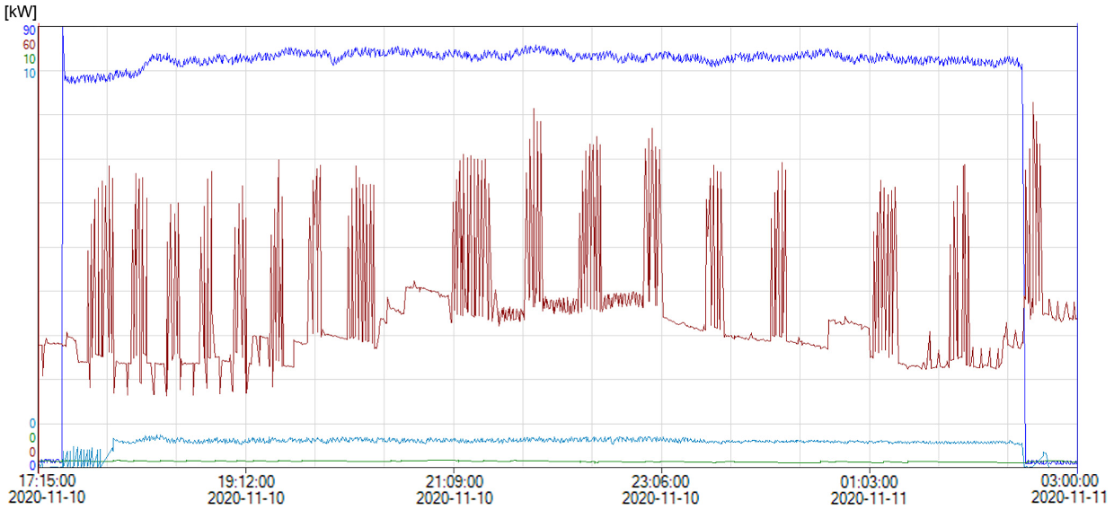
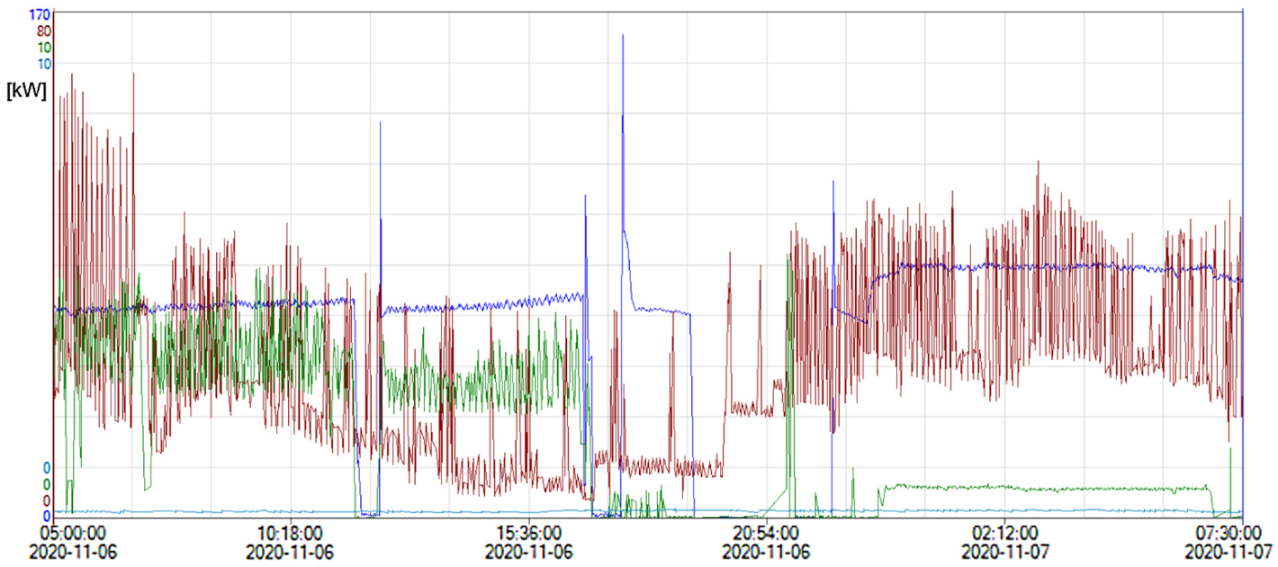
Figure 1 and Figure 2 show examples of the energy consumption in kW during production, acquired from the energy meters of the chosen stages S1, S2, S3, and S4 for the chosen broccoli process with ID 373 and cauliflower process with ID 365. The plots are provided to give example visualizations of the production processes considered in the paper. Let us examine both plots thoroughly.

The energy consumption in kW (vertical y-axis) is presented with the chosen four colors for the stages: S1—brown, S2—green, S3—deep blue, S4—light blue, for both the broccoli and cauliflower production processes. Each stage’s maximum value on the y-axis is given in the upper-left corner of each figure. As we can see, for processes (Figure 1 and Figure 2) with the highest energy consumption, the graphs are very chaotic, but they correspond to events at the production line. Normally, they fluctuate around the average value, but when the temperature of the product drops too much under the desired (optimum) temperature, the energy consumption is reduced for some time. Then, when the temperature of the product rises, the power also increases. At some points, there are planned stops to exchange parts on the lines, e.g., the cutting knives. At these points, we observe zero energy consumption. Then, it surges to 170 kW to return to its average value. The S1 stage shows more chaotic behavior because it is a dynamic cooling chamber. Here, the starts and stops of the compressors are more frequent. This can be seen in both figures. The stages S1 and S4 (before and after the main freezing tunnels) remain at stable levels.

We can see from both figures that it is hard to assess the processes taking into account the current energy consumption. It is very misleading because it corresponds to the normal production flow and its breaking points and milestones. As well as the current energy utilization, the operators and managers must observe the average consumption values, the average production output, the power per ton, and the average power during the whole production process. With these extra data, the management can react properly to production events, e.g., by lowering the output temperature (and raising the energy consumption), increasing the output or reducing it to maintain the optimal CF emission values, and maintaining the parameters of production so that the final product is not rejected.

These cases indicate the research objective, i.e., to build a model that will help in finding relevant production processes with optimal low-emissions factors, and to identify non-optimal processes with both too high and too low energy consumption, incorrect processes due to human error, or processes that are close to optimal but not quite optimal. Hence, we used correlation and clusterization as the main methods. However, how do we know that having properly correlated processes grouped into the relevant groups (described above) results in an optimal and consistent model? The answer lies in the classification methods. These allow us to validate the clusterization groups and choose the proper clusterization method to create a model for a given production process. The other problem is that companies may have only a small quantity of unit processes. In our case, onion production provided us with more than 100 unit processes to create a model to assess other production processes. This is consistent with the theory of unsupervised learning. However, in the case of models for production processes with a lower quantity of unit processes, the proposed method also provides managers with correct models that can support them in managing production, e.g., to achieve low-emissions products.

During the monitoring of the processes, the parameters were measured more thoroughly at stages S1–S5. The whole production process usually lasts 24–36 h and its output is around 20–100 tons of product. During each supervision of the production line in the company, we gathered values (not only average values) of, e.g., the input mass of raw materials and output production assets, the temperatures of the materials, etc. In [22,23], the stage S1 energy consumption was very chaotic, but S3 and S4 had smooth power values except for during the technological breaks described above.

After a year of process measurement, up to the beginning of 2021, there were 104 results collected for frozen onion production and 75 for spinach. The other vegetables had less than 50 cases, e.g., 35 broccoli processes and 42 cauliflower processes. Therefore, the question arose of how to manage and optimize the production in cases with few processes, such as these. Hence, part of the current work presents the results of clusterization. We use onion as the reference product to assess the other vegetable products, i.e., broccoli and cauliflower.

3.5. Assessment of the Production Processes

In order to assess the production line and the product parameters, the company management often uses expert knowledge. Judging by the parameters of the production and product range, experts can identify the proper processes. However, in some factories, the production often lasts for days. For this reason, automatic production assessment is needed to support and manage the production towards optimized products with a low CF.

In this study, we developed a method to demonstrate how to manage the production to achieve low-carbon-emissions products. The reference case study for the production processes consisted of 104 processes (frozen onion production). In this study we applied unsupervised machine learning methods to group the processes according to a scheme that is typical for the industry, i.e., optimal processes, close to optimal processes, far from optimal processes with low and high energy, and processes with incorrectly entered data due to human error.

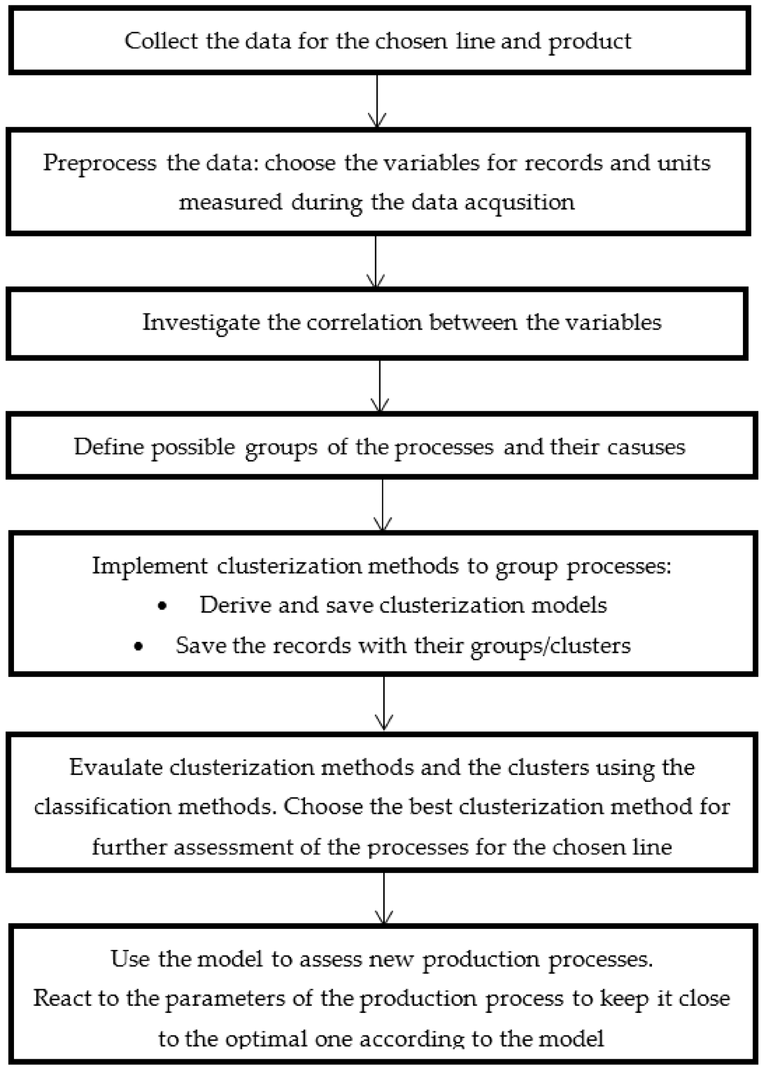
However, companies often use a smaller number of processes for a defined type of product. This fact defines the next step of our study: how to define and apply a methodology to manage production with a limited number of processes. In this paper, we demonstrated how to manage and assess low-emissions processes even if their number was between 30 and 50 and how the company could profit from applying the correlation and machine learning methods used in our methodology. We showed that proper process management, e.g., by raising the average power and the production output capacity, can result in lower energy utilization per ton of the final product. The general outline of the statistical and machine learning methods is shown in Scheme 1.

Let us define the steps of our methodology.

• Collect the data. The data should correspond to the production processes that are stored in the databases, e.g., the energy consumption values from the electric meters, etc. In our case, for the onion production we had five electric power consumption meters. Each of the meters corresponded to one of the production stages S1, S2, …, S5.
• Preprocess the data to obtain the corresponding parameters, factors, units, and values in order to prepare the dataset for further research. In our case, we recalculated the raw data to obtain the average energy consumption of the production stages, the current average production output, and the average energy utilization in one hour (average power).
• Build the correlation matrices to investigate relationships between the energy consumptions of individual technological processes.
• Use unsupervised learning methods. In our case, we chose clusterization methods. As a result, we obtained different models with the data of the processes divided into a chosen number of categories. Each category (cluster) obtained after clusterization was then evaluated to indicate desired processes with a low CF that did not affect the product quality. Some processes with much lower or higher values of the CF at a given stage than those defined by the technology range were examined by the managers.
• Evaluate the processes with the groups/clusters as classes. Some machine learning supervised methods were applied to the data with clusters as classes. The target of this stage of the research was to choose one or two of the best clusterization methods that could be used by the trained clusterization models to assess the subsequent processes.
• Obtain the resulting model for the management and optimization of the chosen production line. In our case, for the onion production, the best model was the k-means model. This was stored to be used for the validation of new processes.
• Validate the current production using the obtained model and provide the production manager with a tool to assess the production process for a given category. The managers may react by setting the optimal parameters, e.g., to lower the production output in order to lower its temperature while maintaining the standard, to raise the power in the freezing tunnel to lower the temperature of the processed materials, or to raise the output when the temperature is lower than required, in order to lower the CF related to production, etc.

3.6. Correlation of the Energy Consumption

In order to investigate the relationships between energy consumption values in individual technological processes for broccoli, cauliflower, and onion processing, correlation matrices were built. These were applied to the data to determine the initial degree of the relationship between the variables.

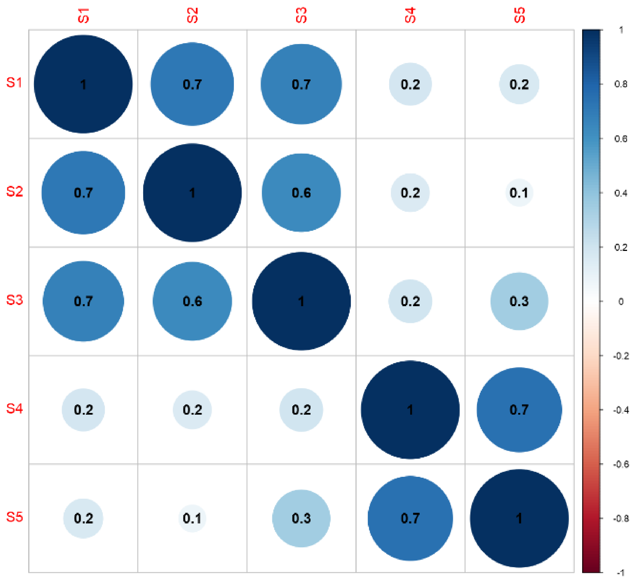
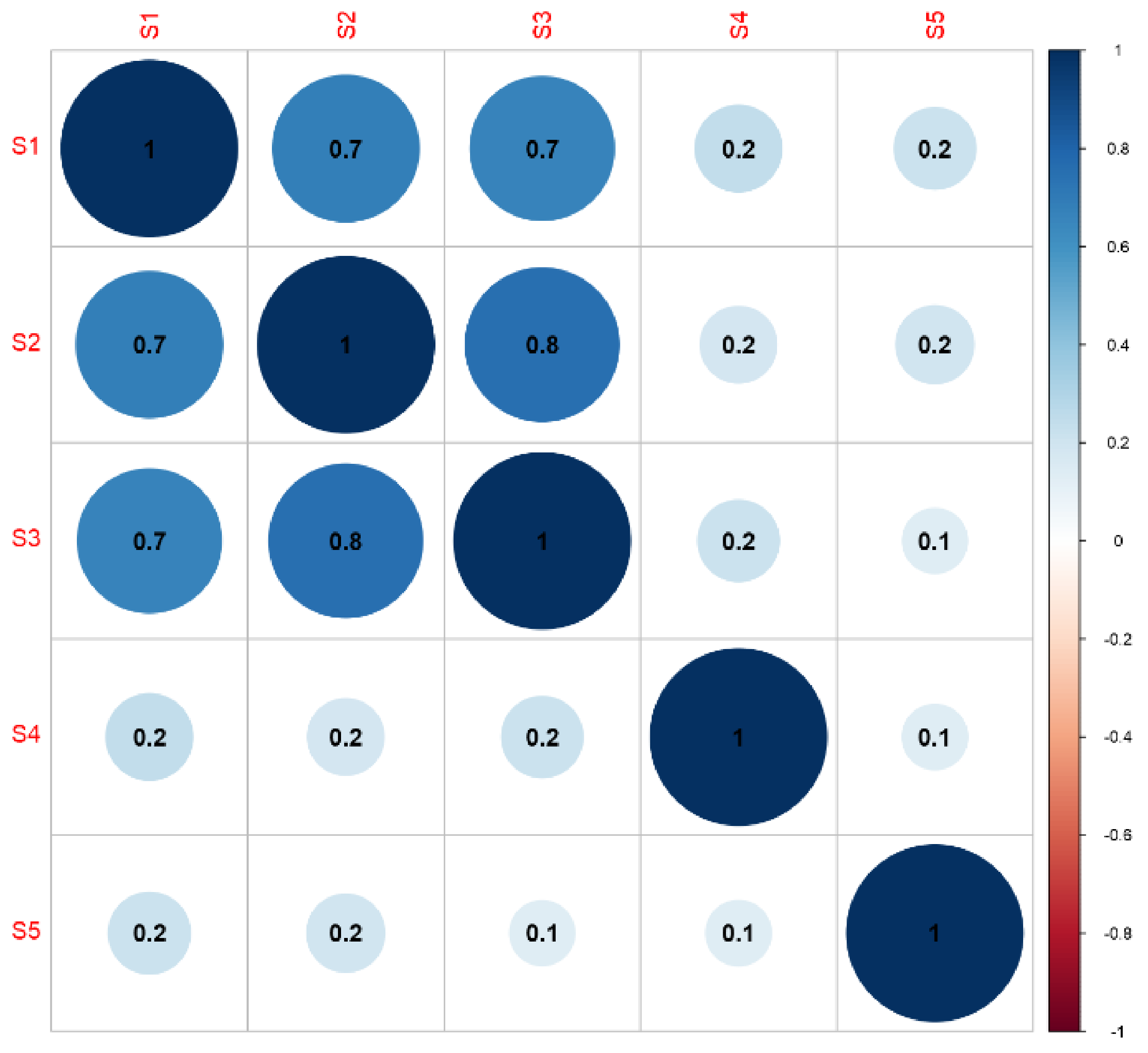
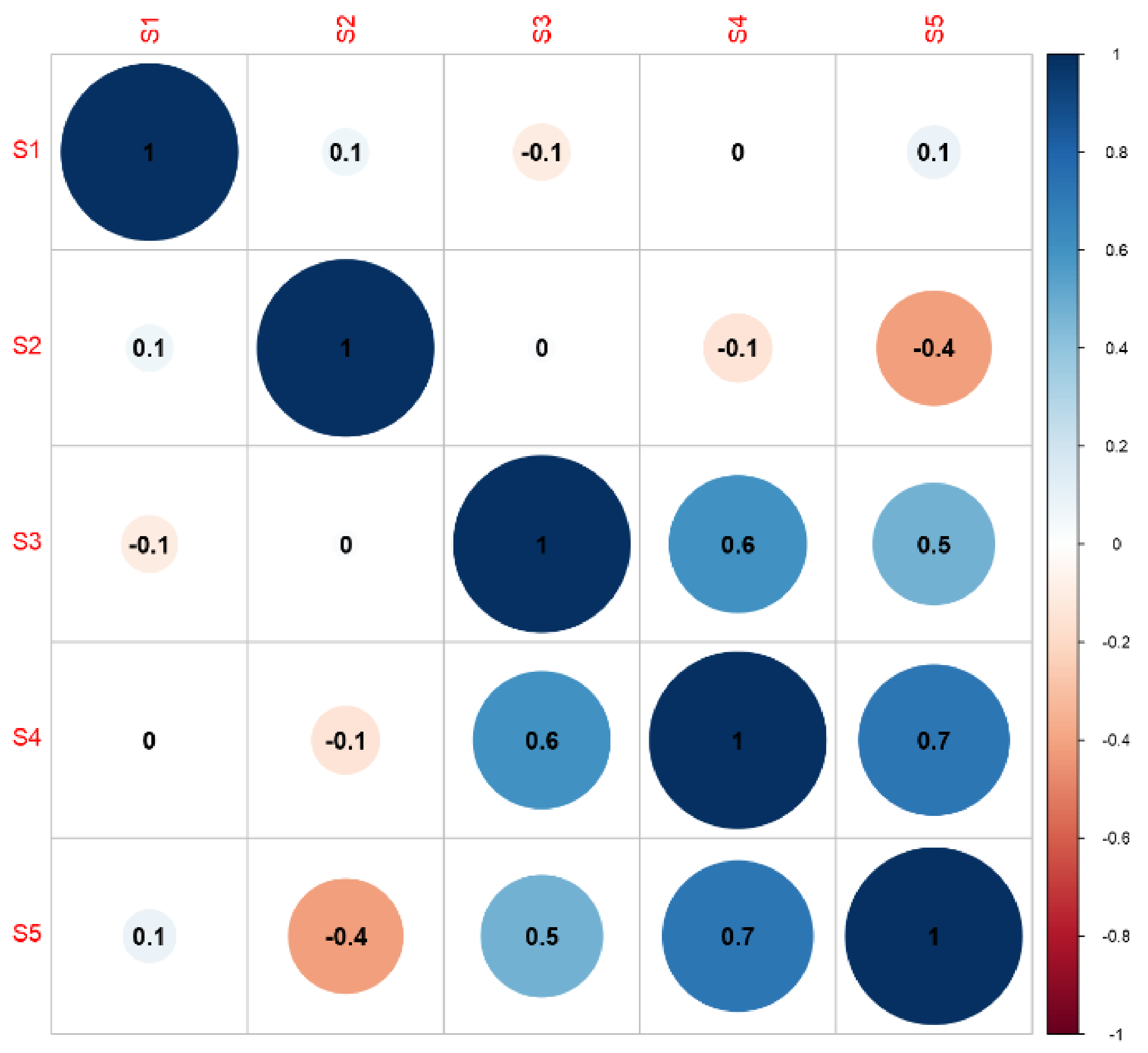
Cauliflower and broccoli are very similar vegetables and therefore have similar processing requirements. The most strongly correlated processes in cauliflower processing were S1 and S2, S1 and S3, S2 and S3, and S4 and S5. The remaining connections can be considered statistically insignificant as the correlation coefficient was too low (Figure 4).

The matrix of correlation of energy consumption at the individual stages of the production of frozen onion showed very strong links between the stages. Low correlation coefficients were only observed in tunnel-related processes (Figure 5).

3.7. Unsupervised and Supervised Machine Learning Methods Used to Assess the Processes

As previously stated, managing production requires the use of automatic production assessment rather than relying on constant expert supervision. Machine learning methods represent one of the solutions to this automatic approach, combining unsupervised and supervised methods. Therefore, in this study, we tested several clusterization (unsupervised) methods and chose three: canopy clustering [29], k-means (KM) [30] and expectation-maximization (EM) [31]. Then, to assess the onion and spinach production processes, the verified dataset was prepared. Moreover, to assess the trustworthiness of the production data, we compared the results of process classification. We validated the unsupervised methods using five classifiers: k-nearest neighbors, multilayer perceptron, C4.5, random forest and support vector machines (SVM) with a radial basis kernel function [30]. These were briefly described in Section 2. All classification and clustering methods were implemented in the Weka library.

Firstly, we show the results for the onion production, which consists of 104 cases. The dataset is big enough to demonstrate and validate the method shown in Scheme 1. After discussion of the onion process, we focus on the study of the broccoli and cauliflower processes using the validated onion method. We start with clustering and then validate the cluster models using classification methods.

First of all, we checked several options with the cluster numbers and chose five clusters for each method that should represent, according to our experience, some of the real-time situations that occur during production and in their accounting systems:

• Optimal production—the product has a temperature from −25 °C to −18 °C at the end of the line.
• Close to optimal—during the high season, production output capacity (kg/h) should be higher; hence the energy consumption should be lower, and the product temperature is allowed to be within the range of −6 °C to −18 °C. It can be close to the optimal production with slightly too high energy consumption or too low energy consumption, resulting in higher energy utilization in a cold store to lower the product temperature.
• Incorrect entering of some parameters, e.g., operator error, resulting in too high or too low results, e.g., for the output capacity.
• Malfunction of the energy meters. This is a different situation from the above and might result in random and unexpected results.

4. Results

Table 3. The canopy clusterization results of the centroids of parameters of the chosen stages. The units for the i-th stage (pS1, S1, etc.) are in kWh/ton for pt and in ton/h for et in kWh/h.

	Onion Clusters Canopy
Attribute	0	1	2	3	4
pS1	0.21	0.24	0.19	0.19	0.26
S1	5.13	6.52	6.19	9.35	6.72
S2	0.07	0.10	0.02	0.07	0.09
pS3	0.01	0.01	0.00	0.01	0.00
S3	1.01	1.46	1.07	1.02	0.92
pS4	1.03	1.68	1.08	0.99	1.20
S4	27.44	35.13	29.06	27.67	24.37
pS5	0.01	0.07	0.01	0.00	0.04
S5	0.18	1.18	0.19	0.01	0.72
pt	2.30	1.48	2.29	2.46	2.77
et	84.28	72.74	90.00	101.01	100.34
instances	28	3	27	33	13

,

Table 4. The k-means clusterization results of the centroids of parameters of the chosen stages.

	Onion Clusters K-Means
Attribute	0	1	2	3	4
pS1	27.82	0.17	0.11	0.74	0.16
S1	53.25	5.97	4.53	3.04	8.07
S2	0.57	0.07	0.06	0.05	0.09
pS3	11.07	0.01	0.01	0.07	0.01
S3	14.19	0.97	1.18	0.61	1.04
pS4	30.38	0.95	0.92	1.79	0.96
S4	32.83	26.47	33.01	8.68	30.46
pS5	0.31	0.01	0.00	0.01	0.02
S5	0.53	0.10	0.09	0.16	0.71
pt	1.86	2.62	2.05	2.10	2.17
et	348.57	93.42	85.38	35.32	90.47
instances	1	42	34	11	16

and

Table 5. The EM clusterization results of the mean values of the parameters of the chosen stages.

	Onion Clusters EM
Attribute	0	1	2	3	4
pS1	0.11	0.16	0.74	27.82	0.16
S1	4.53	8.42	3.04	53.25	5.89
S2	0.06	0.09	0.05	0.57	0.07
pS3	0.01	0.01	0.07	11.07	0.01
S3	1.18	1.03	0.61	14.19	0.97
pS4	0.92	0.96	1.79	30.38	0.95
S4	33.01	30.63	8.68	32.83	26.50
pS5	0.00	0.02	0.01	0.31	0.01
S5	0.09	0.73	0.16	0.53	0.11
pt	2.05	2.15	2.10	1.86	2.61
et	85.38	91.01	35.32	348.57	93.16
instances	37	16	11	1	39

show the reference onion production clusterization.

Table 6. K-means clusterization of broccoli production. The units for the i-th stage (pS1, S1, etc.) are in kWh/ton for pt and in ton/h for et in kWh/h.

	Broccoli Clusters K-Means
Attribute	0	1	2	3	4
pS1	0.08	0.32	0.04	4.19	0.09
S1	1.34	1.35	1.51	4.25	2.08
S2	0.16	0.03	0.23	0.09	0.08
pS3	0.06	0.05	0.03	0.11	0.06
S3	0.91	1.14	0.70	0.21	1.38
pS4	7.68	2.29	0.12	6.54	0.25
S4	49.10	55.69	3.07	13.19	6.40
pS5	0.01	0.18	0.00	0.18	0.01
S5	0.18	1.51	0.03	0.24	0.17
pt	1.56	1.46	1.80	2.11	2.12
et	98.67	91.01	9.91	57.77	20.32
instances	4	4	3	22	2

,

Table 7. Canopy clusterization of broccoli production.

	Broccoli Clusters Canopy
Attribute	0	1	2	3	4
pS1	0.09	0.39	0.08	0.13	0.13
S1	2.85	1.53	0.13	6.92	0.71
S2	0.11	0.03	0.10	0.11	0.05
pS3	0.02	0.06	0.05	0.00	0.07
S3	0.44	1.25	0.63	0.14	0.63
pS4	1.59	1.75	5.22	0.14	5.36
S4	16.85	58.77	45.3	10.65	43.53
pS5	0.01	0.24	0.00	0.00	0.22
S5	0.21	1.74	0.00	0.21	0.42
pt	2.00	1.35	1.55	1.90	1.92
et	42.19	85.69	82.9	33.65	100.1
instances	16	3	3	8	5

,

Table 8. EM clusterization of broccoli production.

	Broccoli Clusters EM
Attribute	0	1	2	3	4
pS1	0.09	0.33	0.02	89.74	0.25
S1	3.17	13.28	1.16	6.92	1.46
S2	0.08	0.11	0.23	0.14	0.06
pS3	0.01	0.02	0.04	2.16	0.06
S3	0.27	0.55	0.77	0.14	1.01
pS4	0.30	1.86	4.55	129.4	3.27
S4	8.60	38.08	20.92	11.29	52.48
pS5	0.01	0.05	0.00	3.61	0.14
S5	0.18	0.68	0.02	0.27	1.02
pt	2.13	2.07	1.71	1.96	1.55
et	26.84	104.9	44.61	465.0	95.07
instances	19	2	5	1	8

,

Table 9. K-means clusterization of cauliflower production. The units for the i-th stage (pS1, S1, etc.) are in kWh/ton for pt and in ton/h for et in kWh/h.

	Cauliflower Clusters K-Means
Attribute	0	1	2	3	4
pS1	0.52	0.18	5.46	6.97	519.2
S1	24.27	2.48	7.08	1.00	2.28
S2	1.13	0.10	0.14	0.06	0.05
pS3	0.17	0.06	0.16	3.20	157.7
S3	8.41	0.97	1.71	0.55	1.21
pS4	0.43	5.22	3.67	22.58	678.1
S4	28.30	57.14	17.50	3.14	5.55
pS5	0.02	0.22	0.14	0.84	48.59
S5	0.69	1.31	0.33	0.06	0.24
pt	1.86	1.37	2.07	1.64	2.22
et	127.0	92.66	79.17	81.15	3332
instances	3	5	17	15	2

,

Table 10. Canopy clusterization of cauliflower production.

	Cauliflower Clusters Canopy
Attribute	0	1	2	3	4
pS1	5.23	0.50	519.2	0.70	0.10
S1	4.52	24.42	2.28	14.62	7.16
S2	0.11	1.60	0.05	0.35	0.08
pS3	1.35	0.09	157.7	0.01	0.01
S3	1.34	8.24	1.21	0.77	2.72
pS4	11.26	0.36	678.1	0.11	0.18
S4	17.43	26.35	5.55	4.30	11.93
pS5	0.42	0.01	48.59	0.00	0.01
S5	0.37	0.55	0.24	0.13	0.58
pt	1.80	1.87	2.22	1.67	1.81
et	83.16	123.6	3332	36.75	44.63
instances	27	2	2	3	8

and

Table 11. EM clusterization of cauliflower production.

	Cauloflower Clusters EM
Attribute	0	1	2	3	4
pS1	3.44	0.50	0.17	34.90	519.2
S1	4.13	23.95	2.13	0.06	2.28
S2	0.10	0.94	0.10	0.00	0.05
pS3	0.11	0.13	0.08	16.03	157.7
S3	1.31	6.59	0.96	0.00	1.21
pS4	2.13	0.34	5.53	113.2	678.1
S4	11.01	22.59	54.4	0.28	5.55
pS5	0.09	0.01	0.19	4.24	48.59
S5	0.23	0.58	1.11	0.01	0.24
pt	1.89	1.94	1.47	1.55	2.22
et	48.6	112.4	94.3	363.0	3332
instances	27	4	6	3	2

show the results of clusterization of the broccoli and cauliflower production processes. The units for the i-th stage (pS1, S1, etc.) are in kWh/ton for the production output capacity (pt) and in ton/h for the average energy consumption (et) in kWh/h.

The results are achieved using five clusters in the chosen clusterization methods and their parameters are defined as follows:

• Canopy: max candidates = 100; periodic pruning = 10,000; min density = 2.0; T2 radius = 0.804; T1 radius = 1.005;
• k-Means (KM) with the Euclidean distance: max candidates = 100; periodic pruning = 10,000; min density = 2.0; T1 = −1.25; T2 = −1.0,
• Expectation-maximization (EM): max candidates = 100; minimum improvement in log likelihood = 1 × 10⁻⁵; minimum improvement in cross-validated log likelihood = 1 × 10⁻⁶; minimum allowable standard deviation = 1 × 10⁻⁶;

Let us discuss Table 3, Table 4 and Table 5 thoroughly to explain the results and show the advantages of the proposed method. The same reasoning is applied to Table 6, Table 7, Table 8, Table 9, Table 10 and Table 11 and these will therefore be discussed briefly. The cluster with ID 4 (denoted later as C4) shows the average values for the stages pS1, S1, S2, pS3, …, pS5, S5, and the production average parameters pt and et as follows: C4 (0.26, 6.72, 0.09, 0.00, 0.92, 1.20, 24.37, 0.04, 0.72, 2.77, 100.34). This means that the optimal process has, e.g., energy consumption at stage S4 equal to 24.37 kW/t, the energy utilized in one hour equal to 100.34 kWh, and thirteen processes that fulfill the conditions of production. As can be seen by summing the values from pS1 to S5, the average energy consumption per ton of the product is equal to 34.32 kW/t and the production output has the highest value, at 2.77 t/h.

Therefore, let us summarize clusterization. Clusterization divides the data into groups and provides us with the centroids (average values) for each group (category). We can assume that the average or centroid values refer to the center of the group and they can be regarded as the reference model of the group.

Hence, clusterization into five clusters provides us with five processes that represent the production process division described earlier, i.e., optimal process, close to optimal but with lower values, close to optimal but with higher values, etc.

We can also conclude, for the reference onion production process, that the division of processes into five clusters by the three clusterization methods shows that:

• The corresponding clusters for the three chosen methods are very similar:

  ○

  Canopy C0, KM C3, EM C3,

  ○

  Canopy C1, KM C4, EM C4,

  ○

  Canopy C2, KM C1, EM C2;

• The clusters have different numbers of instances;
• Their mean values or the centers of the centroids have similar values for the clusters with more than five instances;
• Some clusters could be combined into one, e.g., C0 and C2 in the k-means case, C0, and C4 in the canopy case;
• The optimal cluster for a given clusterization method should show low energy at the cooling stages, but not minimal energy.

The canopy clusterization results show that Cluster 0 has a lower output of 2.30 ton/h and the lowest preprocessing values, but it is the first choice as the optimal process (see Table 3). Cluster 1 has too low an S4 stage energy. The possible cause is incorrect accounting in the system by the operator. Cluster 2 has too high an energy consumption at stages S1 and S4, and lower output. Cluster 4 has the highest production output capacity and lower energy consumption. Cluster 4 occurs during the high season. The processes 201, 2426, and 2388 have too high an energy consumption at the preprocessing stages pS1 and pS4. Cluster 3 has a high value of S4 but is the second choice for the optimized process cluster.

In the k-means results (Table 4), Cluster 0 (C0) has very high energy consumption. A possible cause is erroneous data, because it also has a high preprocess energy consumption for the stages pS1, pS3, and pS4. Cluster 1 is the first choice for an optimal process cluster because it has reasonable energy values for the freezing stages and low energy consumption in other stages, with values of (0.17, 5.97, 0.07, 0.01, 0.97, 0.95, 26.47, 0.01, 0.10, 2.62, 93.42). This gives an average energy consumption per ton equal to around 35 kwh/t. Cluster 2 is the second choice as the optimal process. Cluster 4 has too high an initial freezing stage. Cluster 3 has an S4 stage value that is too low.

In the expectation-maximization method (Table 5), Cluster 0 has reasonable values and is the second choice for the optimal process. Cluster 1 has an initial freezing stage that is higher than optimal. Cluster 2 has S4 values that are too small. Cluster 3 shows values that are too high due to an incorrect entry to the system. Cluster 4, i.e., C4 (0.16, 5.89, 0.07, 0.01, 0.97, 0.95, 26.50, 0.01, 0.11, 2.61, 93.16) is the first choice, as its preprocess values are relatively low, as well as the energy utilization values at the freezing stages.

As previously mentioned, the number of processes for the cases of broccoli and cauliflower production were low, i.e., 35 and 42, respectively. According to our experience, this is rather too low. There is a question of whether it is possible to apply the method derived for the reference production to a case with a low number of production processes and achieve a reliable model to assess new production processes. We show that it is possible, and the proposed method is highly validated by the classification methods.

We can apply the clusterization methods and compute correlations supporting the conclusions by taking into account the onion case. Table 6, Table 7 and Table 8 show the clusterization results for the broccoli processes and Table 9, Table 10 and Table 11 for the cauliflower processes.

For the broccoli case, we can also conclude that for the canopy method (Table 3), clusters zero (C0) and three (C3) can be combined. Together, they would then be similar to the C3 for k-means (Table 4) and C0 for EM (Table 5) clusterizations. The results show a higher divergence than in the onion case due to the number of processes. Nonetheless, the choice of the five clusters is supported.

In the cauliflower case (Table 6), we can see that for the k-means method, cluster three (C3) seems to be the optimal cluster due to the high output capacity and the low freezing stages, providing average (centroid) values of C3 (4.19, 4.25, 0.09, 0.11, 0.21, 6.54, 13.19, 0.18, 0.24, 2.11, 57.77). The canopy clusters C3 and C4 (optimal) for the broccoli case can be combined (Table 7), because they show very close values. Together, they would then be similar to the C2 for k-means and C4 for EM (Table 8) clusterizations.

As in the broccoli case, the results for the cauliflower case (Table 9, Table 10 and Table 11) show a higher divergence than in the onion case due to the number of processes. Nonetheless, they support the choice of five clusters. Table 9 shows that the optimal group for k-means clusterization is C2 with the values (5.46, 7.08, 0.14, 0.16, 1.71, 3.67, 17.50, 0.14, 0.33, 2.07, 79.17). Table 10 shows that cluster 4 for the canopy method has the optimal values (0.10, 7.16, 0.08, 0.01, 2.72, 0.18, 11.93, 0.01, 0.58, 1.81, 44.63). The same can be concluded for the EM clusterization for cluster zero C0 (3.44, 4.13, 0.10, 0.11, 1.31, 2.13, 11.01, 0.09, 0.23, 1.89, 48.6). Nonetheless, the method supports our thesis that the clusterization method can support the management of the production process towards low-emissions products.

To assess and choose the clusterization method, we used five machine learning classification methods. All the clusterization results were assessed by the classification methods with the same input features and class labels resulting from the applied clustering methods.

Table 12. The assessment of clusterization of the onion case using the five chosen machine learning methods.

Classifier	Accuracy of Classification [%]
	Canopy	KM	EM
3NN	98.7	98.0	87.5
C4.5	98.0	99.3	98.7
MLP	92.1	97.4	89.5
RF	100	100	100
SVM	96.1	96.7	88.8

,

Table 13. The assessment of clusterization of the broccoli case.

Classifier	Broccoli Evaluation Results [%]
	Canopy	KM	EM
3NN	85.7	97.1	97.1
C4.5	94.3	100	97.1
MLP	97.1	94.3	97.1
RF	100	100	100
SVM	100	100	100

and

Table 14. The assessment of clusterization of the cauliflower case.

Classifier	Cauliflower Evaluation Results [%]
	Canopy	KM	EM
3NN	90.5	90.5	85.7
C4.5	95.2	97.6	97.6
MLP	92.9	81.0	92.9
RF	100	100	100
SVM	100	100	100

show the classification results of the onion production processes using the following classifiers:

• 3NN (kNN) 3-nearest neighbors;
• Multilayer perceptron (MLP) with a hidden layer with 16 nodes for both production processes with a learning rate equal to 0.79 and momentum equal to 0.39 [13];
• Binary tree C4.5 with a confidence factor equal to 0.25, with the minimum number of instances per leaf equal to 2;
• Random forest (RF) with the bag size percentage equal to 100, with unlimited maximum depth, a number of execution slots equal to 1, and 100 iterations;
• Support vector machine (SVM) with a radial basis function (RBF) given by Equation (5).

K(x,y) = exp(−0.05*(x-y)^2)

(5)

Table 12 shows the results for the onion production as the reference product. It can be concluded that the division into five clusters indicates that the best results are for k-means clusterization, followed by canopy.

Table 13 and Table 14 show the assessment of the production processes for broccoli and cauliflower using the same classification methods as in the onion case. For the broccoli case, the assessment of the EM clusterization shows the highest values, close to 100%. In the case of cauliflower production, the canopy algorithm is the best clusterization approach.

The best derived models for onion production, as well as for broccoli and cauliflower production, as applied to the current production, allow the production management to achieve low-emissions reference models. These models, applied to new production processes that usually last 20–40 h, will support the technicians and managers with a tool to manage the production properly, avoid overuse of power, and react to the changes in the production conditions.

5. Discussion

The authors’ methodology shown in Diagram 1 is supported by the results for the onion production, with more than one hundred unit processes. The results achieved by implementing the methodology, shown in Figure 5 and Table 3, Table 4 and Table 5, show that the reference model/approach for the onion production supports the methodology consisting of correlation, clusterization, and validation by the chosen machine learning methods. The application of the approach used in production processes with a much smaller number of unit processes, i.e., broccoli and cauliflower, is also supported, since:

• The correlation matrices in Figure 3 and Figure 4 show similar relationships to the reference production presented in Figure 5.
• All the chosen clusterization methods provide results (Table 6, Table 7, Table 8, Table 9, Table 10 and Table 11) corresponding to the onion production.
• The validation methods also support the chosen methodology (Table 13 and Table 14), and their results are consistent with those of the reference production (Table 12).

In summary, Table 12, Table 13 and Table 14 indicate that the best clusterization method is k-means for the reference production and the broccoli case. In the case of the cauliflower production, canopy also shows promising results, as demonstrated by slightly worse multilayer perceptron validation results compared with k-means in that production process. In the method used, the production processes were divided into five groups that are typical in the industry, i.e., optimal processes, close to optimal processes, far from optimal processes with low and high energy, and processes with incorrectly entered data due to human error. The clusterization methods were suitable for modeling the problem of division into clusters/groups and solving the problem. From the wide variety of machine learning methods, we chose three clusterization algorithms, after the initial tests.

6. Conclusions

In production management, managers often encounter the problems of how to optimize production, assess the processes, determine the optimized processes, etc. The method presented in this paper and applied to the management of frozen vegetable production showed solutions to these problems. The method is based on statistical and machine learning methods. It can support the management of production lines in order to achieve low-emissions products. We elaborated and tested the methodology for production management. The methodology was based on initial assessment of the production by correlation, then clustering the processes into five groups. Moreover, the clustering was evaluated by five supervised machine learning methods to choose the best algorithm for a given production process.

Unsupervised machine learning methods were used to group the processes according to a scheme that is typical in the industry, i.e., optimal processes, close to optimal processes, far from optimal processes with low and high energy, and processes with incorrectly entered data due to human error. Because companies also have processes with a smaller number of cases, in the next step we showed how to manage and assess low-emissions processes even if the number is between 30 and 50. Due to the limited number of processes, these are not easily managed in a low-emissions context.

Our research to find the best clusterization methods for the purpose was narrowed down to three algorithms: canopy, k-means, and expectation-maximization. The clustering process was validated using five supervised machine learning classification methods: k-nearest neighbors (kNN), multilayer perceptron (MLP), binary tree C4.5, random forest (RF) and support vector machine (SVM). These allowed the best optimal clusterization method to be determined. As the clusters, we chose five groups of processes according to a scheme that is typical in the industry, i.e., optimal processes, close to optimal processes, far from optimal processes with low and high energy, and processes with incorrectly entered data due to human error. In the next step, the method was verified on the onion production line, which has 104 processes, and then applied to production lines with a smaller number of cases. Based on the onion production as the reference, we showed how to manage and assess the low-emissions production when the number of production records was small. In this research, k-means was the best method for clustering the onion processes into five groups, with a validation accuracy >97.4% for the MLP method and equal to 100% for RF. For processes with a small number of cases, k-means also was the best-validated method with an accuracy greater than 94.3% for MLP and equal to 100% for RF and MLP. For the similar cauliflower production, the results indicated canopy clustering as the best method, with a validation accuracy >90.5% for kNN and equal to 100% for RF and MLP, as in the broccoli case.

The research showed that proper process management, utilizing the knowledge from the proposed method, e.g., by raising the average power and the production output capacity, can result in lower energy utilization per ton of the final product. We compared the parameters of ongoing processes with the obtained cluster centroids and modified them towards the optimal group centroid. The comparison was performed using the Euclidean distance between respective vectors of the parameters.