Method to Evaluate the Resistance–Capacitance Voltage Divider and Uncertainty Analysis

Abstract

The resistance and capacitance parameters of a resistance–capacitance divider may change due to factors such as long-term operation, internal insulation flashover, and dielectric breakdown, which will affect the measurement characteristics of the resistance–capacitance divider. Since it is difficult to separate the voltage divider, and because improper disassembly will damage the insulation of the equipment, measuring the resistance and capacitance parameters of a voltage divider non-destructively has always been a problem. In this paper, an indirect method for evaluating the resistance and capacitance parameters is proposed, and the uncertainty of measurement of this method is determined. Simulation and actual test results show that this method can be used to estimate the resistance–capacitance parameters and has a good level of measurement accuracy. Besides, through the uncertainty analysis, it is concluded that the proposed method can overcome measurement errors within a certain range and has high practicability. Finally, a very practical application scenario of the proposed method is given, showing that the proposed method has good economic significance.

1. Introduction

The voltage divider is the key piece of equipment in high-voltage direct current (HVDC) transmission systems. It is mainly used for voltage measurement and provides voltage signals to secondary protection and related devices [1,2,3,4,5]. There are two representative DC voltage measuring devices, namely, the resistance voltage divider and the resistance–capacitance voltage divider [6,7]. Under normal circumstances, the resistance–capacitance-type divider is usually used to prevent component breakdown caused by uneven local voltages in the resistance voltage divider under the impulse voltage scene [8,9]. Each branch of the voltage divider has the same resistance–capacitance time constant to ensure linear frequency response characteristics [10]. The accuracy of a voltage divider is typically assessed at the time of laboratory installation, by comparing it with another voltage divider which has greater accuracy and can be traced back to the National Laboratory [11]. Since it is difficult to separate the voltage divider, and because improper disassembly will damage the insulation of the equipment, measuring the resistance and capacitance parameters of a voltage divider which is put into operation has always been a problem.

However, the resistance and capacitance parameters of DC voltage dividers may change due to internal insulation flashover and dielectric breakdown during their operation. For example, when the capacitance element of the high-voltage arm breaks down under conditions of overvoltage due to insulation defects, the equivalent capacitance value of the high-voltage arm will increase. Wu dismantled a faulty voltage divider and noticed that the capacitance component was broken down, which decreased the secondary output voltage of the voltage divider [12]. Liang found an internal insulation flashover in the DC voltage divider which changed the resistance and capacitance values of the voltage divider and distorted the secondary side voltage [13]. Li analyzed the reasons for electronic equipment failure and external insulation of the DC divider [14]. Wang analyzed the reasons for abnormal secondary voltage of the DC divider [15]. They all came to the same conclusion that the status of the DC voltage divider needs to be checked frequently.

At present, there are few reports on methods to measure resistance–capacitance parameters of resistance–capacitance voltage dividers, and most of these studies are about capacitance dividers. Song studied the capacitance measurement and dielectric loss measurement of the capacitor voltage divider when the divider is connected with the electromagnetic unit [16]. Luo introduced experiences and measures to reduce test errors for on-site insulation dielectric loss measurement [17]. Cui put forward the key content of the work for preventive and test procedure and summarized a feasible method for the judgment of the insulation status [18]. Chen put forward a capacitance measurement method that can be completed without disconnecting the lead wire. In this method, the upper end of the high-voltage arm is grounded, and the lower end is connected to the test voltage. The capacitance of the high-voltage arm is measured by using the Schering bridge. To improve the measurement accuracy, other coherent loops need to be screened [19]. A method of self-excitation was proposed for capacitor voltage transformers with no intermediate voltage outlet. This only applies to capacitor voltage transformers with an electromagnetic voltage and is not suitable for traditional voltage dividers [20]. Ma established a broadband equivalent circuit model of the UHV capacitive voltage transformer based on the impedance parameters and verified the accuracy and effectiveness of the model by comparing the broadband impedance simulation results with the measured results [21].

It can be seen that most of the measurement methods for voltage dividers are measured after the resistance and capacitance components are disassembled, respectively. Although the measurement method is accurate, it is prone to insulation damage and causes other problems in the process of disassembly, which is not conducive to long-term use of voltage dividers. Therefore, this paper proposes a measurement method of resistance–capacitance parameters of voltage divider without disassembly and analyzes the measurement uncertainty of this method.

2. Measuring Principles

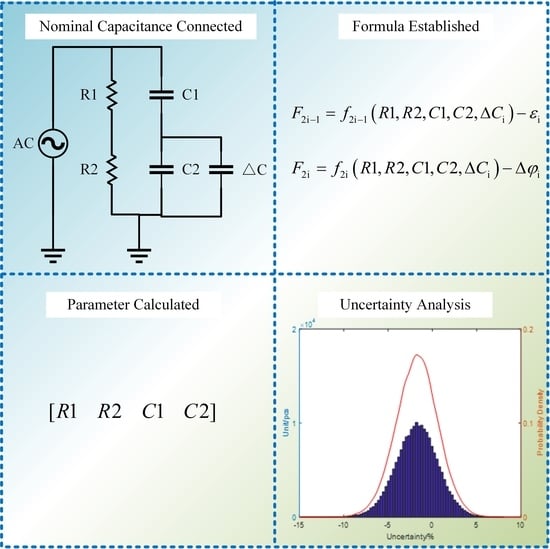
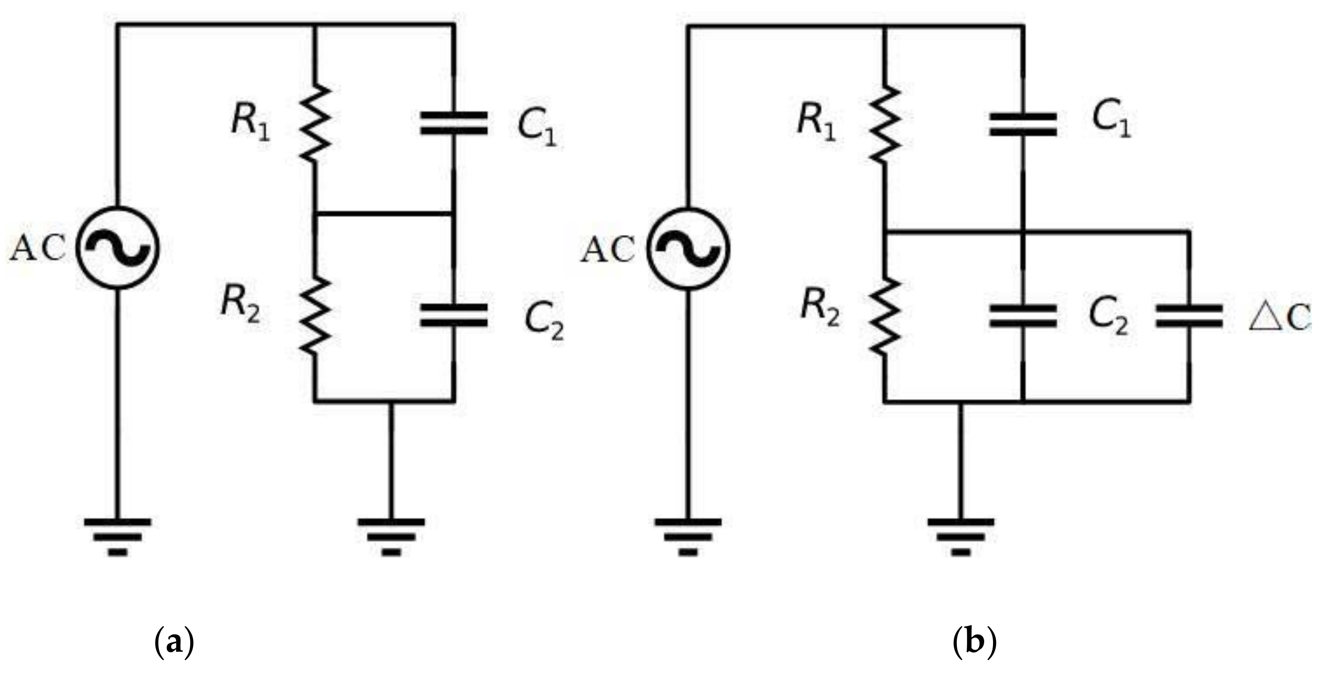
The resistance–capacitance voltage divider is equivalent to the circuit model shown in Figure 1a.

According to the principle of circuit, the impedance parameters of the high- and low-voltage arm are as follows:

$$Z_1=\frac{R_1}{1+j\omega R_1{C}_1}$$

(1)

$$Z_2=\frac{R_2}{1+j\omega R_2{C}_2}$$

(2)

Before the voltage divider produces, both resistance and capacitance are adjusted to the standard value R_1n, R_2n, C_1n, C_2n. The product of R_1n, C_1n and R_2n, C_2n is the same to ensure linear frequency response characteristics [10]. The standard ratio transfer function of the voltage divider is shown as follows.

$$k_{\mathrm{n}}=\frac{Z_{1\mathrm{n}}}{Z_{1\mathrm{n}}+Z_{2\mathrm{n}}}=\frac{R_{1\mathrm{n}}}{R_{1\mathrm{n}}+R_{2\mathrm{n}}}$$

(3)

When the resistance–capacitance parameters of the voltage divider change, the actual voltage divider ratio transfer function is as follows:

$$k^{\prime }=\frac{Z_1}{Z_1+Z_2}$$

(4)

The measuring principles of the method proposed in this paper are to derive the resistance and capacitance parameters of the voltage divider by measuring the frequency response of the voltage divider at 50 Hz through the measuring model, i.e., the voltage divider ratio transfer function.

The frequency response of the resistance–capacitance voltage divider under the power frequency can be tested on the spot using the frequency test source and the standard resistance voltage divider. The standard resistive voltage divider acts as a reference for the ratio difference in the frequency response without introducing any phase angle changes. The ratio difference ε₁ and the angle difference ∆φ₁ of the voltage divider ratio are measured. ε₁ and ∆φ₁ should be as follows:

$${\epsilon }_1=\frac{\mathrm{abs}\left(k^{\prime }\right)-k_{\mathrm{n}}}{k_{\mathrm{n}}}$$

(5)

$$\Delta {\phi }_1=\mathrm{angle}\left(k^{\prime }\right)$$

(6)

where abs(*) and angle(*) represent the amplitude operator and phase angle operator of the complex number parameter, respectively.

Since the ε₁ and ∆φ₁ can be measured directly by frequency response test equipment [22], two equations are obtained with four unknown variables. In order to calculate all the unknown variables, two or more equations are needed.

Therefore, a nominal capacitance ∆C of known value is connected in parallel in the low-voltage arm to change the frequency response of the system. The circuit model is shown in Figure 1b. The frequency response test of the resistance–capacitance voltage divider is carried out again using the same method. The ratio difference ε₂ and the angle difference of the voltage divider ∆φ₁ can be obtained. The C₂ changes to C₂ + ∆C in ε₂ and ∆φ₂, which is different from ε₁ and ∆φ_1.

$${\epsilon }_2=\frac{\mathrm{abs}\left(k^{\prime }\right)-k_{\mathrm{n}}}{k_{\mathrm{n}}}$$

(7)

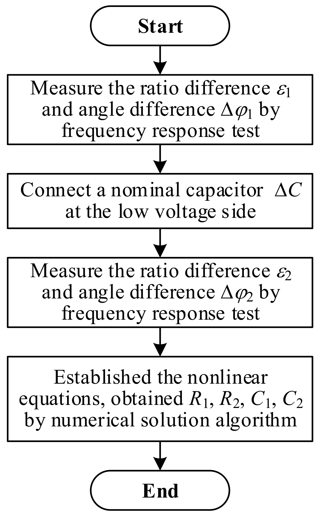
$$\Delta {\phi }_2=\mathrm{angle}\left(k^{\prime }\right)$$

(8)

By combining Equations (1)–(8), we can obtain four quaternion cubic equations. Using common solving algorithms, we can solve four unknowns, R₁, R₂, C₁, and C₂. The steps for this method are shown in Figure 2.

We cannot accurately measure the actual ratio difference, angle difference, and the nominal capacitance; that is to say, there is a measurement error in ε₁, ε₂, ∆φ₁, ∆φ₂, and ∆C. It has been verified that when a certain error is large enough, the error of the resistance and capacitance will surge, and even make the equation unsolvable. Therefore, the proposed method needs to be further improved.

3. Fitting Algorithm

Since the equations may not be solvable due to errors, the authors propose an optimization method to solve the equations and increase the number of equations.

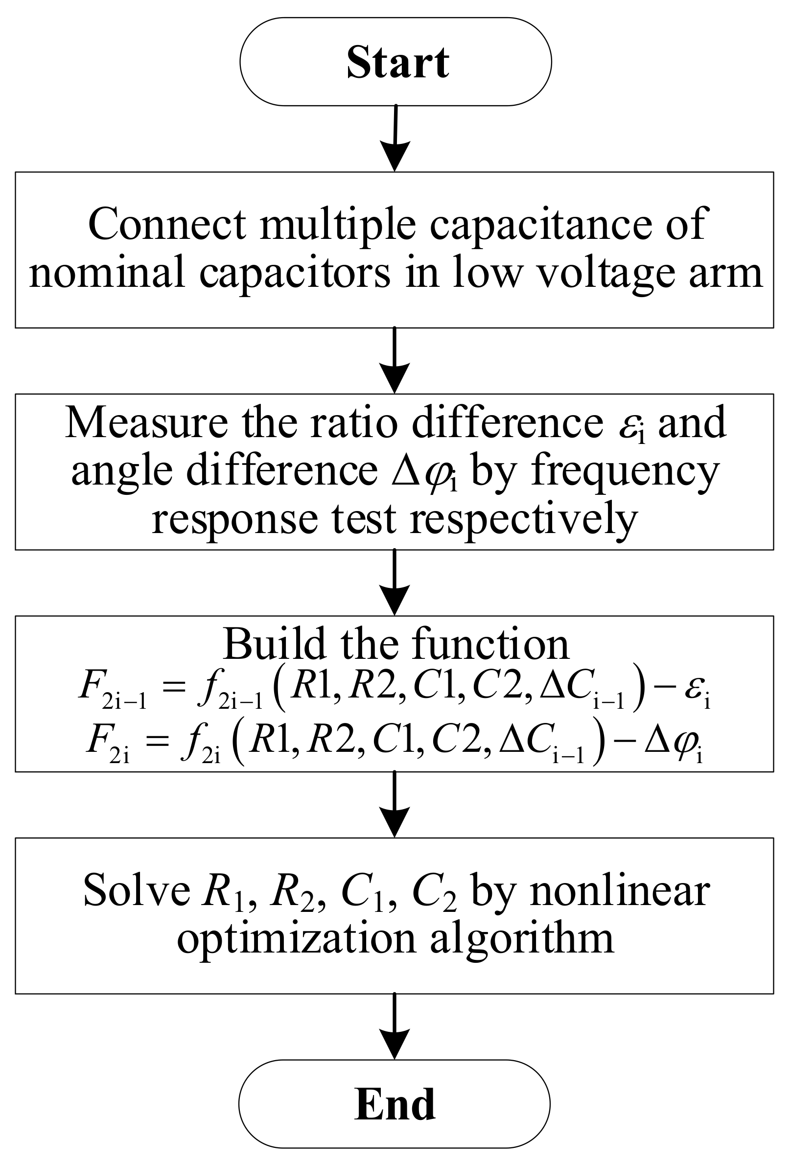
More nominal capacitors can be connected in parallel on the low-voltage arm to obtain more quaternion cubic equations. The unknown parameters of R₁, R₂, C₁, and C₂ can be estimated with numerical solution algorithms such as nonlinear optimization. The expressions are as follows:

$${\epsilon }_{\mathrm{i}}=f_{2\mathrm{i}-1}\left(R_1,R_2,C_1,C_2,\Delta C_{\mathrm{i}}\right)$$

(9)

$$\Delta {\phi }_{\mathrm{i}}=f_{2\mathrm{i}}\left(R_1,R_2,C_1,C_2,\Delta C_{\mathrm{i}}\right)$$

(10)

where i = 1, 2, 3, …, n, and ∆C₁ = 0. Suppose the following function,

$$F_{2\mathrm{i}-1}=f_{2\mathrm{i}-1}\left(R_1,R_2,C_1,C_2,\Delta C_{\mathrm{i}}\right)-{\epsilon }_{\mathrm{i}}$$

(11)

$$F_{2\mathrm{i}}=f_{2\mathrm{i}}\left(R_1,R_2,C_1,C_2,\Delta C_{\mathrm{i}}\right)-\Delta {\phi }_{\mathrm{i}}$$

(12)

where ε_i, ∆φ_i, ∆C_i are known quantities, and R₁, R₂, C₁, and C₂ are unknown quantities.

This problem can be transformed into an optimized solution for the following nonlinear least-squares problem:

$$\min \frac{1}{2}{\displaystyle \sum _{\mathrm{i}=0}^{\mathrm{n}}{‖F_{\mathrm{i}}‖}_{\mathrm{m}}}$$

(13)

In Equation (14), ${‖F_{\mathrm{i}}‖}_{\mathrm{m}}$ is the p norm, which is defined as follows:

$${‖F_{\mathrm{i}}‖}_{\mathrm{m}}={\left({\displaystyle \sum _{\mathrm{i}=1}^{\mathrm{n}}{\left|F_{\mathrm{i}}\right|}^{\mathrm{p}}}\right)}^{\frac{1}{\mathrm{p}}}$$

(14)

Through i experiments, 2i F_i can be obtained. Numerical solution algorithms, such as the steepest descent method, Newton method, Gauss–Newton method, Levenberg–Marquardt method, and other nonlinear optimization methods can be used to estimate the four unknowns of R₁, R₂, C₁, and C₂ to measure the resistance and capacitance parameters of the power divider. The steps for this method are shown in Figure 3. For the case study, see Section 5.1.

4. Uncertainty Evaluation

As mentioned in Section 3, there is a measurement error in ε₁, ε₂, ∆φ₁, ∆φ₂, and ∆C, which will lead to error in the measurement results of resistance and capacity parameters. The measurement error is caused by the inaccurate measurement device and the different environmental conditions.

In this section, a reasonable method is selected to quantify the measurement error of the resistance and capacitance parameters.

According to the existing international standards, there are two uncertainty analysis methods, namely the GUM method and Monte Carlo method [23]. As the measurement model proposed in this section is nonlinear, it is difficult to use the traditional GUM method. Therefore, the Monte Carlo method is selected in this paper to evaluate the uncertainty variation range of output results when each input quantity changes.

The Monte Carlo method is a numerical method that achieves distribution propagation through repeated sampling. It is a method that uses random sampling of the probability distribution to carry out distribution propagation. The idea for solving the problem is to establish the probability model to be solved so that the solution to the problem is exactly the same as the mathematical expectation or has other characteristic quantities of the probability model built. Then, multiple simulations are performed to calculate the probability of an event or the estimated parameters.

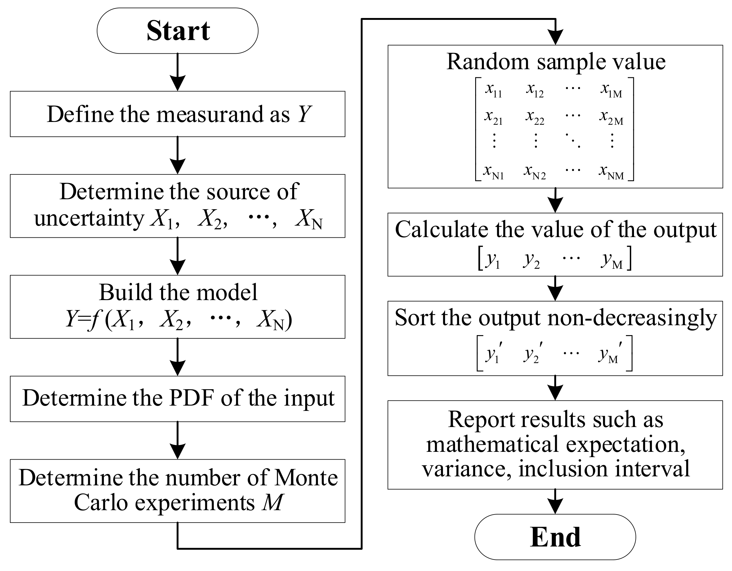
The Monte Carlo method uses discrete sampling of the probability density function (PDF) of the input quantity X_i, spreads the distribution of the input quantity from the measurement model, calculates the discrete sampling value of the PDF of the output quantity Y, and then directly determines the discrete distribution value of the output quantity to obtain the best estimates of the output, the standard uncertainty, and the inclusion interval of the agreed inclusion probability. The specific implementation steps are as follows:

(1)

Define the required measurement as output Y;

(2)

Determine the source of the uncertainty of the output, denoted as the input quantity X₁, X₂, …, X_N;

(3)

Establish the relationship between the output quantity Y and the input quantity of the measurement model Y = f (X₁, X₂, …, X_N);

(4)

Determine the PDF of each input according to the actual situation;

(5)

Determine the number of Monte Carlo experiments M;

(6)

Extract M sample values x_ir from the PDF of the input quantity X_i;

(7)

Substitute the input quantity samples into the output quantity model, and calculate the corresponding output value;

(8)

Carry out non-decreasing sorting on the obtained discrete output value;

(9)

Construct a report of the uncertain evaluation results, including the mathematical expectation, variance, and inclusion interval.

The whole process is shown in Figure 4.

In this paper, the quantities to be measured are the ratio difference ε_i, the angle difference ∆φ_i, and the nominal capacitance ∆C_i. These quantities should be used as inputs for the uncertainty evaluation. The output is the error between the resistance and capacitance parameters (R₁, R₂, C₁, and C₂) of the power divider and their actual measurement results. Through the Monte Carlo experiment on the distribution of the input quantity, the distribution of the output quantity is obtained. For the case study, see Section 5.2.

5. Case Study

5.1. Algorithm Study

As described in Section 2, multiple nonlinear equations can be obtained by paralleling nominal capacitors of different sizes in the low-voltage arm many times. Then, the values of R₁, R₂, C₁, and C₂ can be obtained by using the nonlinear optimization algorithm.

In this study, the sequential quadratic programming (SQP) algorithm was used to solve the nonlinear optimization problem. The solution model was built and verified. The verification process used was as follows.

(1)

Measure the actual values of R₁, R₂, C₁, and C₂ by direct measuring method;

(2)

Calculate the actual ratio difference and angle difference of the resistance–capacitance divider under the conditions of no paralleling nominal capacitance, paralleling 30 nF nominal capacitance, paralleling 60 nF nominal capacitance, paralleling 90 nF nominal capacitance, and paralleling 120 nF nominal capacitance of the low-voltage arm;

(3)

Measure the actual ratio difference and angle difference [22], and obtain the calculated values of R₁, R₂, C₁, and C₂ through the calculation of this model;

(4)

Compare the deviations between the calculated and measured values of R₁, R₂, C₁, and C₂.

The measured values of R₁, R₂, C₁, and C₂ were 20.02 MΩ, 2.002 kΩ, 439.6 pF, and 4344 nF, respectively. Following the steps above, five groups of capacitors were connected in parallel, and the ratio difference and angle difference of the system were measured, as shown in

Table 1. Ratio difference and angle difference in the actual situation.

Value of Parallel Capacitance/nF	Ratio Difference/%	Angle Difference/%
0	1.165	0.121
30	0.443	0.046
60	−0.177	−0.018
90	−0.887	−0.092
120	−1.533	−0.159

.

After substituting the parallel nominal capacitance value, the measured ratio difference, and the angle difference value into the solution model, the values of R₁, R₂, C₁, and C₂ were calculated, as shown in

Table 2. The results of the model.

	R1	R2	C1	C2
Measured Value	20.02 MΩ	2.002 kΩ	439.6 pF	4344 nF
Calculated Value	19.66 MΩ	1.965 kΩ	443.5 pF	4383 nF
Error	−1.8226%	−1.8246%	0.8900%	0.9021%

. Their respective deviation values were also calculated.

It can be seen that under the actual working conditions, the deviation between the actual values of R₁, R₂, C₁, and C₂ and those calculated by this model was not large, and the deviations of capacitance and resistance were within 1% and 2%, which is acceptable.

In this case, the nominal capacitance value rather than the measured value of the four parallel capacitance is adopted, since measurement of the standard substance would reduce its accuracy in use. However, there is still a difference between the nominal value and the actual value. These factors and the measurement error of frequency response all affect the calculation results, but the final calculation results show that the proposed method can overcome measurement errors within a certain range and has high practicability.

5.2. Uncertainty Evaluation Method Study

In this part, a case study of the uncertainty evaluation method is given based on the case given in Section 5.1.

In this case, fifteen inputs were included in the uncertainty analysis, namely, the nominal capacitances ∆C₁, ∆C₂, ∆C₃, and ∆C₄; the ratio differences ε₁, ε₂, ε₃, ε₄, and ε₅; and the angle differences ∆φ₁, ∆φ₂, ∆φ₃, ∆φ₄, and ∆φ₅. Among them, ∆C₁ represented the case where the low-voltage arm was not connected in parallel, and its value was 0, following a single-point distribution. The PDF of other input parameters should be studied.

The uncertainty levels of nominal capacitance were determined using the B-Type uncertainty method, i.e., the probability distribution of inputs is determined by calibration certificates [23]. The calibration certificate of the nominal capacitance indicates that the expanded uncertainty of the standard substance is 0.4% (k = 2). The PDF of nominal capacitance is determined as normal distribution with standard deviation 0.2%.

The uncertainty levels of the ratio difference and the angle difference were determined using the A-Type uncertainty method, i.e., the probability distribution of inputs is determined by multiple independent repeated measurements [23]. In this case, the uncertainty of the ratio difference and the angle difference obtained through 20 measurements was about 0.1%. The PDF of the ratio difference and the angle difference was determined as normal distribution with standard deviation 0.1%.

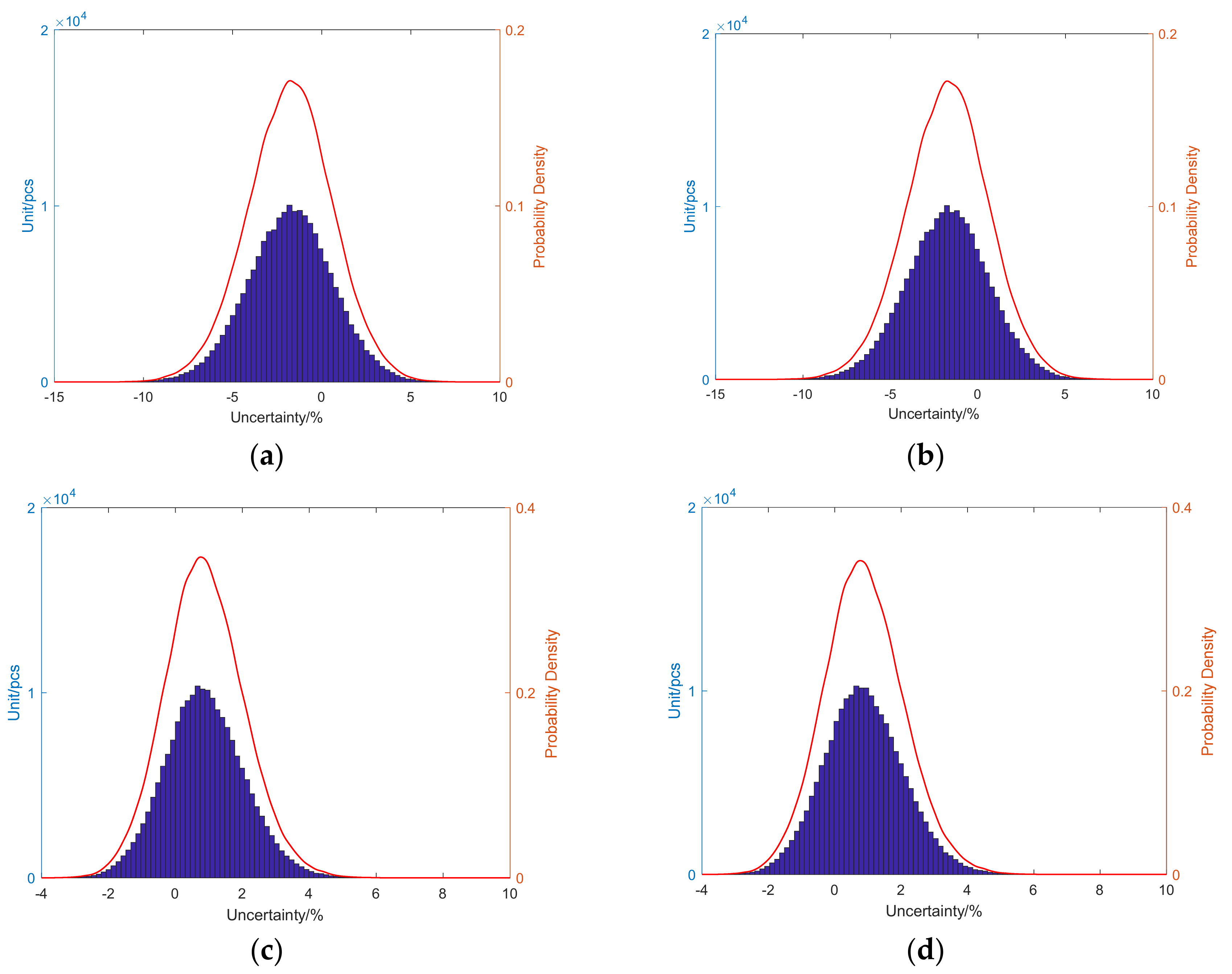
The Monte Carlo method was used to conduct 200,000 simulations. The blue and red parts of Figure 5 show the frequency distribution histogram (FDH) and probability density function (PDF) of each output.

Table 3. Confidence interval width under single-input uncertainty conditions.

	R1	R2	C1	C2
Average Value/%	−1.769	−1.750	0.869	0.877
Standard Deviation/%	2.375	2.354	1.182	1.197
Lower Bound of Interval/%	−6.449	−6.414	−1.456	−1.476
Upper Bound of Interval/%	2.926	2.878	3.200	3.242

shows the distribution characteristics of the deviation of the output, including the average value, standard deviation, and 95% confidence interval.

When the measurement uncertainty of the nominal capacitance, ratio difference, and angle difference was considered at the same time, the deviations in the values of R₁, R₂, C₁, and C₂ calculated by this model were not large. The deviations in values of the resistance and capacitance were within 2% and 1%, respectively, and the uncertainty was within 3%. The 95% confidence interval was also within a reasonable range.

It is worth noting that the voltage divider resistance and capacity parameters do not change during the whole Monte Carlo simulation process. What has changed is the measurement error of each input. The magnitude of variation of each input is determined by the A-Type or B-Type uncertainty assessment method. This evaluation method can basically simulate the actual application situation. After tests in Section 5.1 were repeated many times, it was found that all results fell within its 95% confidence interval, which further verified the effectiveness of the Monte Carlo evaluation method.

5.3. The Influence of Each Input on the Measurement Result

The influence of the measurement uncertainty of the nominal capacitance, ratio difference, and angle difference on the output has great significance for the selection of the measurement meter in practical applications.

This case uses the uncertainty evaluation method in Section 5.2 to analyze the variation of the 95% confidence interval width of output under different input uncertainty. The uncertainty of each input was [0.001, 0.002, 0.003, 0.004, 0.005], and when studying the influence of single-input uncertainty on the output error uncertainty, the uncertainty of the other inputs was set to 0.

The length of the confidence interval for the output error uncertainty under single-input uncertainty is shown in

Table 4. Ratio difference and angle difference in the actual situation.

Input	Input Uncertainty/%	Confidence Interval Width/%
		R1	R2	C1	C2
Nominal Capacitance	0.1	2.052	2.035	1.060	1.07
	0.2	3.478	3.452	1.848	1.875
	0.3	3.910	3.879	2.051	2.080
	0.4	3.881	3.849	2.028	2.056
	0.5	4.938	4.888	2.608	2.640
Ratio Difference	0.1	9.396	9.311	4.671	4.729
	0.2	17.047	16.879	8.420	8.531
	0.3	24.612	24.375	12.098	12.269
	0.4	31.965	31.711	15.733	15.918
	0.5	38.871	38.513	19.325	19.529
Angle Difference	0.1	5.635	5.575	2.828	2.854
	0.2	5.639	5.583	2.795	2.827
	0.3	5.862	5.808	2.873	2.912
	0.4	6.109	6.061	2.955	2.994
	0.5	6.493	6.433	3.062	3.106

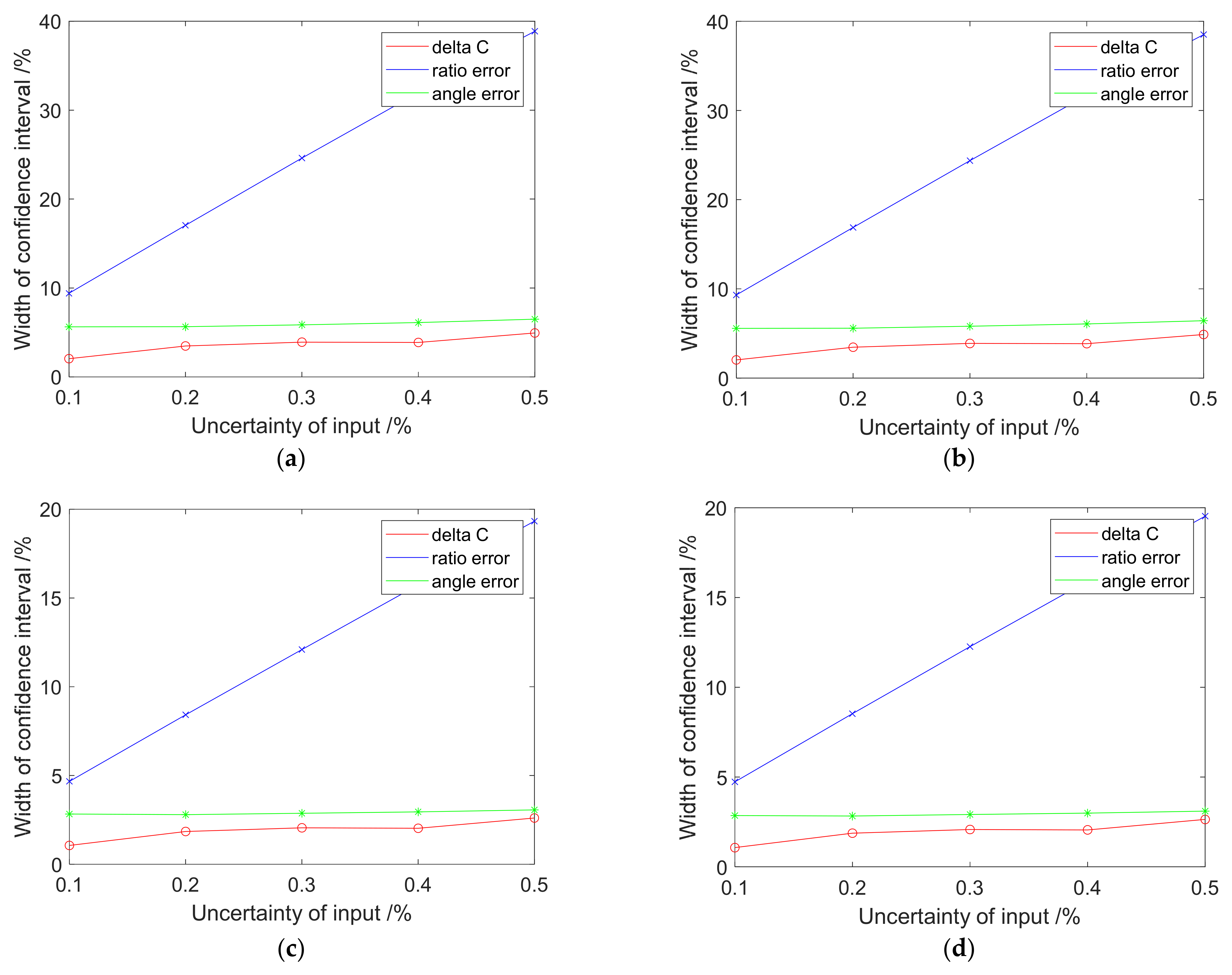
. In this case, R₁, R₂, C₁, and C₂ were used as examples to study the variation trend for the length of confidence interval for the output error uncertainty with single-input uncertainty, as shown in Figure 6. The results show that when the input uncertainty increased from 0.1% to 0.5%, the length of the confidence interval for each output showed an increasing trend. When the ratio difference uncertainty was taken as the input, the range of variation in the confidence interval length was the largest. When the nominal capacitance or angle difference uncertainty was taken as input, the confidence interval length was relatively small.

The results provide a reference for the selection of practical measuring instruments. First, it is recommended that a higher accuracy meter is used or the number of measurements is increased when measuring the ratio difference to reduce measurement uncertainty. Second, when selecting the nominal capacitance or measuring angular difference, relatively low-accuracy meters can be used to reduce test costs.

6. Application Scenarios

The application scenario of the measurement method proposed in this paper is of high practical value. After measuring the resistance and capacitance parameters of the faulty voltage divider in operation, the high- and low-voltage arm elements can be compensated to keep them still in use rather than being scrapped.

Since the high-voltage arm of the resistance–capacitance voltage divider has been packaged and cannot be modified, it is necessary to compensate by changing the resistance and capacitance of the low-voltage arm after calculating R₁, R₂, C₁, and C₂. When the resistance divider ratio is different from the rated transformation ratio, it is recommended that the low-voltage arm resistance components should not be modified on-site. Correspondingly, the proportional coefficient of the back-end merging unit should be adjusted to correct the overall voltage divider ratio so as not to affect the performance of the voltage divider in its other functions. After that, the capacitance value of the low-voltage arm and the compensation capacitance ∆C′ are calculated using (15) and (16), respectively:

$$C_2^{\prime }=\frac{R_1{C}_1}{R_2}$$

(15)

$$\Delta C^{\prime }=C_2^{\prime }-C_2$$

(16)

Generally, the capacitance of the high-voltage arm becomes larger after being broken down, and a parallel capacitor (∆C′ > 0) is required to achieve capacitance compensation. If ∆C′ < 0 is solved, the capacitance of the low-voltage arm can only be replaced with a value of C₂′ to compensate for the frequency response characteristics.

7. Results

In this paper, a method to evaluate the resistance–capacitance voltage divider is proposed. In this method, multiple nominal capacitors are connected in parallel on the low-voltage arm of the resistance–capacitance divider, and the ratio difference and angle difference of the partial voltage ratio are measured. R₁, R₂, C₁, and C₂ are estimated and calculated by the nonlinear optimization algorithm to avoid removing parts or disconnecting the lead wire for field measurements. The analysis results also show that the proposed method can overcome measurement errors within a certain range and has high practicability.

In addition, a Monte Carlo method is selected in this paper to quantify the measurement error of the proposed method. Through the case study, the feasibility of the evaluation method is verified. It can also be concluded that using instruments with relatively low accuracy can be appropriate when selecting nominal capacitance or measuring angular difference, which can reduce the cost of measuring instruments while ensuring measurement accuracy.

Besides, a very practical application scenario of the proposed method is given. After measuring the resistance and capacitance parameters of the faulty voltage divider in operation, the high- and low-voltage arm elements can be compensated to keep them still in use rather than being scrapped.

References

- Tang, G.F.; He, Z.Y.; Pang, H. Research, application and development of VSC-HVDC engineering technology. Autom. Electr. Power Syst. 2013, 37, 3–14. [Google Scholar]
- Zhang, S.H.; Zhou, Y.F.; Li, D.Y. On-site calibration test of ±800 kV converter station DC potential transformer. High Volt. Technol. 2011, 37, 2119–2125. [Google Scholar]
- Liu, J.; Ye, Y.J.; Hu, J.H. Principle and insulation structure analysis of the 800 kV DC voltage measuring device. Power Syst. Clean Energy 2019, 39, 158–167. [Google Scholar]
- Hrbac, R.; Kolar, V.; Bartlomiejczyk, M.; Mlcak, T. A development of a capacitive voltage divider for high voltage measurement as part of a combined current and voltage sensor. Elektron. Ir Elektrotech. 2020, 26, 25–31. [Google Scholar] [CrossRef]
- Fang, Z.; Luo, Y.; Zhai, S.; Qian, B.; Liao, Y.; Lan, L.; Wang, D. Temperature Rise Characteristics and Error Analysis of a DC Voltage Divider. Energies 2021, 14, 1914. [Google Scholar] [CrossRef]
- Kovacevic, U.D.; Stankovic, K.D.; Kartalovic, N.M. Design of capacitive voltage divider for measuring ultrafast voltages. Int. J. Electr. Power Energy Syst. 2018, 99, 426–433. [Google Scholar] [CrossRef]
- Koviljka, S.; Uroš, K. Combined measuring uncertainty of capacitive divider with concentrated capacitance on high-voltage scale. IEEE Trans. Plasma Sci. 2018, 46, 2972–2978. [Google Scholar]
- Zhang, R.Y.; Chen, C.Y.; Wang, C.C. High Voltage Test Technology; Tsinghua University Press: Beijing, China, 2002. [Google Scholar]
- Fei, Y.; Wang, X.Q.; Wang, B.J. Selection and development of ±1000 kV UHV DC transformer. High Volt. Technol. 2010, 36, 2380–2387. [Google Scholar]
- Li, K. Research on Voltage Measurement Device of ±1100 kV UHVDC Voltage Transformer and Its On-Line Monitoring System; Huazhong University of Science and Technology: Wuhan, China, 2017. [Google Scholar]
- Brandao, A.F.; Da Silva, I.P.; De Silos, A.C.; Ivanov, D.; Dias, E.M. On Site Calibration of Inductive Voltage Transformers. In Proceedings of the 8th WSEAS International Conference on System Science and Simulation in Engineering, Genova, Italy, 17–18 October 2009. [Google Scholar]
- Wu, D.W.; Zhou, H.G. Analysis of breakdown in capacitance voltage divider component of 500 kV CVT. Power Capacit. React. Power Compens. 2011, 32, 74–76, 79. [Google Scholar]
- Liang, X.M.; Chang, Y.; Wu, J.K. Internal fault analysis of high voltage direct current transmission DC voltage divider with anti-accident measures. Autom. Electr. Power Syst. 2012, 36, 118–121. [Google Scholar]
- Li, G.G.; Song, J.H.; Pi, J. Analysis on HVDC voltage abnormal fluctuation of Niuzhai-Conghua DC transmission system. Electr. Meas. Instrum. 2019, 56, 82–87. [Google Scholar]
- Wang, Q.; Tan, B.Y.; Liu, Q.S. Anomalous cause analysis of secondary voltage in DC voltage ivider for ±800 kV Converter Station. Hydropower Energy Sci. 2017, 35, 204–207. [Google Scholar]
- Song, S.L. Capacitance and Dielectric Loss Measurement of Capacitor Voltage Divider. Power Capacit. React. Power Compens. 2002, 4, 35–42. [Google Scholar]
- Luo, J.C.; Song, S.L. Research on Insulation Dielectric Loss Measurement of Capacitor Voltaae Transformer. Transformer 2012, 6, 39–46. [Google Scholar]
- Cui, Z.J.; Zhang, Q.M. Discussion About the Understanding of the CVT Dielectric Loss Tangent tan δ Pilot Test Standard. Smart Grid 2014, 10, 46–50. [Google Scholar]
- Chen, L.J. 220 kV Capacitive Voltage Transformer without Disassembling the Lead to Measure the Dielectric Loss and Capacitance Comparison of Different Wiring Methods. Autom. Appl. 2020, 4, 112–114. [Google Scholar]
- Zhang, Z.J. Self-excitation test method for capacitive voltage transformers without intermediate voltage leads. Electr. World 2011, 6, 39–41. [Google Scholar]
- Ma, Q.Y. Impedance Measurement and Parameter Sensitivity Analysis for Ultra High Voltage Capacitor Voltage Transformer. High Volt. Eng. 2014, 6, 1828–1838. [Google Scholar]
- Zhai, S.L. Field Test Power Supply and Test Method for Frequency Response of DC Voltage Divider. Southern Power System Tech. 2021, 15-8, 87–94. [Google Scholar]
- International Organization for Standardization. Uncertainty of Measurement Part 3: Guide to the Expression of Uncertainty in Measurement (GUM:1995); Supplement 1: Propagation of distributions using a Monte Carlo method, TS ISO/IEC GUIDE 98-3-2015; ISO, ISO Copyright Office: Geneva, Switzerland, 2015. [Google Scholar]