Optimisation of the Two-Tier Distribution System in Omni-Channel Environment

Abstract

This paper deals with the problem of the design and configuration of a distribution system that supports the delivery of goods to customers using various commercial channels. In this sense, a modelled distribution system, called an omni-channel distribution system, should ensure the delivery of the same products in different ways while guaranteeing its highest efficiency. The authors propose a single-criterion mixed-integer programming model for the configuration of a complex distribution system of goods in an omni-channel environment. A minimized cost function, composed of key logistics elements including transport, warehouse location, and manipulation processes, is the objective function. The model was experimentally verified, and as a result, potential savings of around 5–8% of the omni-channel design distribution system costs versus the multi-channel distribution system costs were identified. In the paper, an extended sensitivity analysis is also performed to show how specific parameters of the model can change the final recommendation.

1. General Consideration

1.1. Omni-Channel Context of a Distribution System

The dynamic increase in sales realized through online channels has reached a constantly high rate and some authors recognize this trend as global, see, e.g., Biggs and Suhren [1]. The global trend is driven not only by an increase in sales in existing electronic channels but also by the fact that growing numbers of traditional retailers have been entering into e-commerce. Recently, this phenomenon has vastly intensified, mainly due to the COVID-19 pandemic and the resulting radical change in customer behaviour. As a consequence, retailers need effective distribution systems to serve their customers through several commercial channels at the same time, see Hübner et al. [2].

Despite the ongoing trends in the electronic channels, traditional solutions cannot be neglected. Therefore, it is necessary to search for solutions that allow maintaining the sustainable development of transport and distribution systems within the everchanging market conditions. This has become very important recently and hence efforts are made globally to replace combustion engine vehicles used by the freight transport market with alternative fuel vehicles, mainly with electric vehicles (EV). This can be seen as an attempt to create energy-efficient forms of transport.

While this trend is highly recognised in passenger cars and light commercial vehicles, there are still some barriers to EV adoption in the heavy-duty commercial vehicles, including lower driving ranges and long charging time.

Taking all these limitations in the development of transport and distribution systems into account, it seems reasonable to constantly search for organizational solutions to minimize its negative environmental and social impacts. Therefore, it is necessary to configure distribution systems in such a way as to make better use of the existing potential, i.e., on the one hand, to reduce the costs of delivery and, on the other hand, to minimize the effects of transport on the environment. In this paper, the problem of the design, configuration, and parameterization of a distribution system capable to effectively serve customers through several alternative commercial channels is considered.

Up to now, few terms and definitions have been developed for the commercial context, including multi-, cross-, and omni-channel, which are used interchangeably. However, several authors, e.g., Beck and Rygl [3] and Hübner et al. [2], argue that the distinction among them is still not clear. Each of these channels has certain features and advantages, but a single channel is not suitable for all situations (Yadav et al. [4]), which is presented in detail by Chopra [5]. For the purpose of this paper, the authors have adopted the definition of omni-channel proposed in Brynjolfsson et al. [6] and Abdulkader et al. [7]. Omni-channel retailing is a business model in which the company provides the customers with a seamless experience in which there is no difference between physical and online shopping. In contrast, multi-channel retailing is a business model in which the operator provides the customers with the flexibility to use different channels to obtain products or services. Thus, it is concerned with delivering a product through several channels that are operated separately.

The research presented in this paper is concentrated on the design and configuration of distribution systems that are under the control of one operator. The customer, i.e., the final recipient of goods, receives all the requested products using the available types of commercial channels in an optimal way.

1.2. State-of-the-Art Distribution System Using Several Commercial Channels

Some of the first studies in the field of distribution system design come from the 1970s and 1980s. They focused on the facility location problem (e.g., Geoffrion and Graves [8], Geoffrion et al. [9], Gelders et al. [10]). Since that time, very extensive exploration in that research area has been conducted. Special attention is paid by Klose and Drexl [11] to capacity constraints (capacitated vs. incapacitated models), the complexity of system structure (single vs. several tier), the variety of distributed products (single vs. several), the volume of demand, dynamism (static vs. dynamic models), the level of demand (historical vs. forecasted), etc. Generally, a series of review papers in the field of optimization of distribution systems reveal numerous publications dealing with location facilities in a distribution system (Klose and Drexl [11], Laport et al. [12]), supply chain configuration (Melo et al. [13], Farahani [14]) or the practical implications of the applied optimisation procedure (Mangiaracina et al. [15]).

At the beginning of this century, some authors, e.g., Swaminathan and Tayur [16], suggested that e-commerce can significantly change the business model of a global commerce and thus become not only the main driver of growth but may also change the design of distribution systems, hence the concept of a distribution system that can serve more than one commercial channel. The literature on distribution system design within the context of more than one commercial channel can be divided into two key issues, including a strategic management-oriented research on channels configuration, e.g., Ishfaq et al. [17], Hübner et al. [2], and the optimisation of multiple channel distribution systems, e.g., Alptekinoğlu and Tang [18], Xie et al. [19], Zhang et al. [20], and Yadav et al. [4].

Within the first group, Ishfaq et al. [17] considered multiple attributes of the physical distribution process to identify the associations with order execution methods adopted by omni-channel retailers. They used a classification tree analysis to identify the associations among distribution attributes, the methods of order execution, and delivery services. Hübner et al. [2], in their research, investigated on how and why retailers with multiple channels transformed their logistics activities into omni-channel systems. They obtained empirical data via an exploratory survey of over 60 international executives from German retail and logistics enterprises. Another example of exploratory analysis is presented by Lim and Srai [21]. Based on a methodology combining empirical methods with case studies, the authors identified powerful relations among key dimensions that constitute the distribution system, including network structure, network flow, relationship governance, and service architecture.

The second group of research, concentrated on the optimisation of distribution systems, may be divided into two key subsets. One of them is devoted to the multi-channel concept and the related distribution system, while the other one deals with the omni-channel concept and its distribution system, see, e.g., Yadav et al. [4].

As far as the multi-channel concept is concerned, Alptekinoğlu and Tang [18] developed a model of a general multi-channel distribution system subject to stochastic demand. The objective of the optimization is to minimize the total expected distribution cost. Alptekinoğlu and Tang tested their multi-channel model with two specific applications. The first one deals with a store-based retailer expanding into a direct sales channel, while the other application intends to combine the distribution systems of two retailers after a potential merger-and-acquisition. In another research, Xie et al. [19] developed a two-stage decision-making process to improve the manufacturing capacity planning and its allocation in the supply chain. Zhang et al. [20], in their paper, proposed a model for designing supply chain networks with multiple channels. They constructed a multiple objective optimisation model that is concentrated on (a) reducing economic cost for supply chain enterprises, (b) improving the flexibility of order execution, and (c) diminishing the environmental impact. They argued that the considered problem was too complex to be solved with exact algorithms and proposed a multi-objective artificial bee colony intelligent algorithm (MOABC).

In the omni-channel context of the optimisation of distribution systems, few systematic literature reviews have been published up to now, see, e.g., Raza and Govindaluri [22], Ya-Jun and Chris [23]. Based on hundreds of papers published in the last 10 years, the authors performed a comprehensive review in this matter. Interestingly, despite the substantial number of papers, there are very few dealing with the optimisation of distribution systems or supply chains.

The common understanding of optimisation in omni-channel context is that both the facility location and product flow are considered inseparably. There are, however, some papers on other specific aspects of omni-channel distribution, including routing (e.g., Abdulkader et al. [7]) or demand allocation between channels (e.g., Shpak et al. [24]). Abdulkader et al. in their research, proposed a variant of vehicle routing problem (VRP) that involves the decision which customers need to be assigned to particular stores based on the availability of merchandise and finding the routes for the respective vehicles. The location of stores in this formulation is fixed. On the other hand, Shpak et al. have proposed two linear optimisation models of the repartition of production between sales channels. The first model is based on profit maximization, while the second one is concentrated on the risk minimisation.

One of the first papers on complex distribution system design with omni-channel environment was proposed in 2017 by Yadav et al. [4]. The authors constructed a multiple criteria mixed-integer programming model for the distribution system. The decision variables were responsible for facility locations (including manufacturers, central and regional depots) directly serving the customers and the product flow between facilities and customers. The authors proposed a bi-objective optimization model, where the first objective is a minimized total supply chain cost (including fixed costs of facility and transportation between facilities), while the second one is a minimized carbon footprint (produced from operating the facilities and the transport itself). The problem was solved with an exact algorithm using CPLEX solver. The authors, however, did not suggest a final solution to the considered problem. In the research of Si et al. [25], special attention was paid to the randomization of the model due to the uncertainty of the customer demand and the high number, i.e., four, of the network levels. They constructed an optimisation location routing model where the objective was to minimize the total cost of the operated network, including variable transportation and, similar to [4], the carbon treatment costs at each network level, and the fixed cost of location. Due to the complexity of the model, a particle swarm optimization (PSO) procedure was applied to solve the problem. A multiple level of the distribution system in an omni-channel context was also considered by Guerrero-Lorente et al. [26]. In the problem formulation, the authors exposed the customers’ preferences while selecting the place where the product is received, i.e., picked up. The problem was formulated by means of mixed integer programming (MIP). However, the location-routing aspect of the problem was simplified by local transport cost estimation. Finally, the problem was solved with specialized heuristic.

One of the last papers on the omni-channel distribution design problem was published by Huang and Shi [27]. In this research, a bi-objective programming model was constructed to minimize the distribution costs from the facilities to recipients, and to minimize the fixed cost of the facility’s location, related to its capacity, demand, and rent fluctuation. The problem was solved by combining programming and elite set multi-objective simulated annealing algorithm iteratively. The procedure was experimentally applied to relocate a set of facilities to serve a substantial number of e-commerce enterprises in Beijing, China.

A detailed review of the analysed works on the omni-channel distribution network design problem allows us to formulate comparative conclusions in several dimensions, including the structure of the distribution network, the nature of the operated commercial channels, the demand profile, the type and key dimensions of the mathematical model, the solution procedure, and the scope of the model’s application. The result of the comparison is presented in Appendix A in the form of

Table A1. A state-of-the-art in the optimisation of the omni-channel distribution network design problem-part 1.

Research			Distribution System (DS)				Commercial Channels			Demand 2
Reference	Decision Problem	Context	Type	Structure of DS			Channels	No. of Products	Tariff
				Actors 1	Location	Capacity
Alptekinoğlu, Tang [18]	Demand assignment	Logistics network design under stochastic demand	2-tier	S, D, C	Defined	Capacitated	Multi-	Single	Single	Stoch.
Zhang et al. [20]	Facility location and product flow	Compromise network design	4-tier	S, P, CD, RD, C	Defined	Capacitated	Multi-	Single	Single	Determ.
Yadav et al. [4]	Facility location and product flow	Comparison between omni-channel and conventional supply chain	4-tier	S, P, CD, RD, C	Defined	Capacitated	Omni-	Single	Single	Determ.
Si et al. [25]	Facility location and product flow	Logistics network design under uncertain demand	4-tier	CD, RD, LD, D, C	Defined	Capacitated	Omni-	Multiple	Single	Stoch.
Guerrero-Lorente et al. [26]	Facility location and product flow	logistics Network design for deliveries and returns	4-tier	CD, RD, LD, D, A	Pre-defined	Capacitated	Omni-	Single (parcel)	Different (per deliveries and returns)	Determ.
Huang, Shi [27]	Facility location	Relocation of the front distribution center	1-tier	D, C	Pre-defined	Capacitated	Omni-	Single	Single	Determ.
This paper	Facility location and product flow	Comparison between omni-channel and multi-channel	2-tier	S, RD, C	Pre-defined	Incapacitated	Omni-	Multiple	Different per product	Determ.

¹ S—Supplier; P—Producer/Manufacturer; CD—Central Depot; RD—Regional Depot; LD—Local Depot; C—Customer; A—Automated Stations; ² Determ.—deterministic; Stoch.—stochastic.

and

Table A2. A state-of-the-art in the optimisation of the omni-channel distribution network design problem-part 2.

Research	Mathematical Model								Solution and Application
	Program. Technique 1	No. of Criteria	Objective Function						Solution Procedure	Area of Application
			Cost Factors 2					Other Criteria
			Transp.	Facil. 3	Invent.	Backord.	Other
Alptekinoğlu, Tang [18]	NLP	1	Yes	No	Yes	Yes	No	N/a	Problem decomposition into single depot sub-network, solved by any convex NLP procedure	2 networks (small)
Zhang et al. [20]	MILP	3	Yes	Yes (f)	No	No	No	Demand coverage; Environmental aspect	MOABC (modified multi-objective artificial bee colony)	3 networks (small, medium, large)
Yadav et al. [4]	MIP	2	Yes	Yes (f, v)	No	No	No	Carbon content caused by facilities and transport	CPLEX	4 networks (different size)
Si et al. [25]	MIP	1	Yes	Yes (f, v)	No	No	Carbon treatment	N/a	CPLEX and improved PCO (particle swarm optimization)	1 network (medium)
Guerrero-Lorente et al. [26]	NMIP	1	Yes	Yes (f, v)	No	No	Penalty and discounts	N/a	MIP-based heuristic	1 network (medium)
Huang, Shi [27]	MIP	2	No	Yes (f)	No	No	Distribution costs	N/a	CPLEX, MOSA (multi-objective simulated annealing)	1 network (medium); region of Beijing
This paper	MILP	1	Yes	Yes (f, v)	No	No	No	N/a	Exact procedure, simplex	1 network (small)

¹ Programming technique, including, MIP—mixed integer programming, MILP—mixed integer linear programming, NLP—nonlinear programming, NMIP—nonlinear mixed integer programming; ² Cost factors, including, Transp.—transportation, Facil.—facility, Invent.—inventory, Backord.—backorders, Other—other cost factors; ³ Facility cost factor, including fixed costs (f) and/or variable costs (v).

. Based on that, several observations are formulated, which are as follows:

• Gross of the researchers formulates the distribution network design problem as the facility location and the flow of products, occasionally as the only facility location or the demand allocation.
• The key research objective discussed by the researchers is to build an optimal structure of a distribution network using a single-criterion approach or to obtain a compromise solution based on a multi-criteria evaluation. A few works compare the benefits of using the omni-channel distribution network in relation to conventional solutions; at the same time, there are no studies showing the benefits of using an omni-channel vs. a multi-channel distribution network.
• The structure of the distribution network considered in the literature is substantially different. It varies from a one-tier model composed of depots and customers to three-and four-tier models composed of suppliers, producers, depots at various operational levels, i.e., from central to local, and customers—either human beings or automatic devices. The location of each facility is usually defined a priori, and it is always with limited capacity. The results of the research presenting models with unlimited capacity of facilities have not been reported.
• Almost all distribution networks being the subject of the literature review consider the supply of single product type, except one case, where a variety of products are referred to.
• In most cases, there is presented in the literature a single, i.e., a unique, transport tariff at each distribution network tier; the exception is reported to one product with different tariffs depending on the type of products’ flow, i.e., one tariff for deliveries and the other tariff for returns. The results of the research with tariff differentiation at the same tier of the distribution network have not been reported.
• The distribution network design problem is modelled by many researchers using various programming techniques, both linear, i.e., MIP or MILP, and non-linear, e.g., NLP or NMIP. The mathematical model is formulated either with single-objective or multiple-criteria model; in each case, the basic and always present dimension is cost-oriented objective. The other dimensions are related to profitability, demand coverage, or environmental aspects. Moreover, the cost-oriented criterion can optionally be expressed in several dimensions, including the cost of transport, the cost of facilities (both fixed and variable costs), the cost of inventory or shortages, the cost of penalties, and price discounts.
• A demand in the analysed distribution networks is, in most cases, deterministic; only two results of the research are referred to stochastic demand.
• To solve the decision problem, single- and multi-criteria heuristic techniques are mostly used by the researchers. The experimental applications of the proposed models are verified on distribution networks of various sizes, considering the number of objects on different levels of this network; the medium-sized cases dominate.

As a result of the above-presented conclusions based on the literature review, a research gap has been discovered. The solution of the omni-channel distribution network design problem should be extended to the following dimensions: the comparison of benefits between omni-channel and multi-channel distribution networks, the design of optimisation models with unlimited object capacity, the consideration of heterogeneous products at different tiers of the distribution network (if relevant) and the focus on different transport tariffs per product (if relevant), the application of stochastic demand, and the application of different techniques to solve the design problem. The proposals of the extensions should provide a wider perspective of the omni-channel distribution network evaluation as well as its design.

1.3. Research Objective

The main objective of the research proposed in this paper is to optimize the structure of the omni-channel distribution network, which fills the identified research gap. The model is unique in the sense of fulfilling the following features:

• It includes the homogeneous product within each considered commercial channel; however, a diversified cargo unit, i.e., transport packaging, is applied;
• It defines the differentiated transport tariffs at each tier of the distribution network—each tariff can depend on the distance and/or the size of the cargo, i.e., transport packaging;
• It assumes an unlimited capacity of all facilities in the structure of the distribution network, and its volume is specified on the basis of optimisation computations;
• It allows the comparison of the benefits of using the omni-channel versus multi-channel distribution network.

The proposed research is also consistent with the assumptions described in the current state-of-the-art; in particular, the following aspects of the network design problem are taken into consideration:

• It is formulated as the facility location and the product flow problem;
• It assumes the multi-tier structure of the distribution network, i.e., a two-tier structure has been adopted, including the configuration of senders, depots, and receivers;
• It expresses the customers’ demand in a deterministic form;
• the mathematical model is formulated as a single criterion with the MILP technique; the objective function reflects the main components of the distribution network operating cost;
• It is applied a precise technique for LP problems solution due to the linear nature of the model and a consideration of a small size distribution network.

2. Methodology

2.1. Notations

In the research, some indices, decision variables, parameters, and objective functions are defined. The list of all of them are presented in the following table, see

Table 1. This list of indices, decision variables, parameters, and objective function in alphabetical order.

Symbol		Definition
Type	Notation
indices	i	– supplier in a distribution system responsible for sending correct quantity of products with respect to available volume, i = 1, 2, …, I
	j	– recipient in a distribution system, an entity whose demand for product is met, j = 1, 2, …, J
	k	– depot, a facility in a structure of a distribution system being located between supplier and recipient, responsible for receiving appropriate quantity of products from the supplier and their resupply to the customer, k = 1, 2, …, K
	p	– commercial channel, i.e., the composition of supply chain, p = 1, 2, …, P
decision variables	xikp, xkjp, xijp	– volume of transported products within a commercial p-channel, from i-supplier to k-depot (i,k), from k-depot to j-recipient (k,j), and from i-supplier to j-recipient (i,j), expressed in (unit)
	ykp	– location of k-depot in a distribution system within a commercial p-channel (-)
parameters	c(l)	– unit transportation cost depended on distance l
	c(q)	– unit transportation cost dependent on load size q, i.e., independent on distance l
	cikp, ckjp, cijp	– transportation cost of a product per unit within p-channel, from i-supplier to k-depot (i,k,p), from k-depot to j-recipient (k,j,p), and from i-supplier to j-recipient (i,j,p); expressed in (MU/unit) 1
	cikp(lik), ckjp(lkj), cijp(lij)	– unit transportation cost rate, dependent on distance (l), within p-channel at (i,k) relation, (k,j) and (i,j) relations, respectively, expressed in (MU/unit⋅km)
	cikp(qikp), ckjp(qkjp), cijp(qijp)	– unit transportation cost rate, dependent on load size (q), within p-channel at (i,k) relation, (k,j) and (i,j) relations, respectively, expressed in (MU/unit)
	Djp	– demand of j-recipient within p-channel; in (units/month)
	$h_{kp}^f$	– fixed storage cost (cost of facility) at k-location within p-channel; in (MU/month)
	$h_{kp}^v$	– variable storage cost (handling and commissioning costs) at k-location within p-channel; expressed in (MU/unit)
	l	– distance defined on a considered relation, expressed in (km)
	lik, lkj, lij	– distance from i-supplier to k-depot (i,k), from k-depot to j-recipient (k,j), and from i-supplier to j-recipient (i,j); expressed in (km)
	rikp, rkjp, rijp	– load conversion rate of unit load size transported within p-channel into the unified load size at (i,k) relation, (k,j) relation, and (i,j), respectively (-)
	Sip	– supply volume of i-supplier within p-channel (unit/month)
	Qkp	– processing capacity of k-depot within p-channel (unit/month)
	$q_{ikp}$$, q_{{}_{ikp}}^{min}$$, q_{{}_{ikp}}^{max}$	– unit load size (current, min and max) in (i,k) relation within p-channel (unit)
	$q_{kjp}$$, q_{kjp}^{min}$$, q_{kjp}^{max}$	– unit load size (current, min and max) in (k,j) relation within p-channel (unit)
	$q_{ijp}$$, q_{{}_{ijp}}^{min}$$, q_{{}_{ijp}}^{max}$	– unit load size (current, min and max) in (i,j) relation within p-channel (unit)
	$q_{{}_{ikp}}^u$$, q_{{}_{kjp}}^u$$, q_{{}_{ijp}}^u$	– unified load size offered in a distribution system, transported in relations (i,k), (k,j), and (i,j), respectively, of a commercial p-channel (unit)
objective function and components	F	– minimized cost of transportation and storage, expressed in (MU)
	T	– total transportation cost, expressed in (MU)
	TSD	– transportation cost of load movement between the supplier and depots (MU)
	TDR	– transportation cost of load movement between the depots and recipients (MU)
	TSR	– transportation cost of load movement between the suppliers and recipients (MU)
	W	– total storage cost, expressed in (MU)
	WD,f	– fixed cost of a depot, i.e., real estate cost (MU)
	WD,v	– variable cost of storing and handling process at depot, i.e., processing cost (MU)

¹ MU—monetary unit.

.

2.2. Key Analytical Assumptions

The logical model of the considered omni-channel distribution system is presented in Figure 1. Here, a two-tier distribution system is described with respect to four key dimensions (indices), including a finite list of i-suppliers (i = 1, 2, …, I), j-recipients (j = 1, 2, …, J), k-depots (k = 1, 2, …, K), and p-channels (p = 1, 2, …, P). The decision variables, i.e., the volume of transported products within the omni-channel, are represented by x_ikp, x_kjp, and x_ijp.

The analytical assumptions for constructing the optimization model of the two-tier omni-channel distribution system are as follows:

• A one-operator of the distribution system with minimum two types of operated commercial p-channels is considered;
• A list of alternative locations of i-suppliers is defined a priori; their supply volume S_ip is unknown;
• A list of alternative locations of k-depots is defined a priori; their capacity, Q_kp, is not defined;
• A location of each j-receiver and its demand within commercial p-channel is known and defined a priori;
• A homogenous product is assumed for each commercial channel, represented by a type of cargo unit, e.g., a EUR-pallet, pack, cartoon, or returnable container;
• A distance between two points in a considered network, i.e., l_ik, l_kj, and l_ij, is calculated using a typical shortest path procedure;
• Only the forward distribution is considered, i.e., returns (backflows) are omitted.

2.3. Decision Variables and Objective Function

The mathematical model of the considered decision problem is formulated as a mixed-integer programming model and is presented in this section. The cost-oriented minimised objective function F is composed of transportation costs T, resulting from cargo movement between the supplier and depots T^SD, between the depots and recipients T^DR, between the suppliers and recipients T^SR, and storage costs W, including fixed cost of a depot, i.e., real estate costs W^D,f, and variable costs of storage and manipulations, i.e., processing costs W^D,v. It is represented by the following Equations (1)–(6):

$$F=\min (T+W)=\min (T^{SD}+T^{DR}+T^{SR}+W^{D,f}+W^{D,v}),$$

(1)

where:

$$T^{SD}={\displaystyle \sum _{i=1}^I{\displaystyle \sum _{k=1}^K{\displaystyle \sum _{p=1}^P{c}_{ikp}·r_{ikp}}}}·x_{ikp},$$

(2)

$$T^{DR}={\displaystyle \sum _{k=1}^K{\displaystyle \sum _{j=1}^J{\displaystyle \sum _{p=1}^P{c}_{kjp}·r_{kjp}}}}·x_{kjp},$$

(3)

$$T^{SR}={\displaystyle \sum _{i=1}^I{\displaystyle \sum _{j=1}^J{\displaystyle \sum _{p=1}^P{c}_{ijp}·r_{ijp}}}}·x_{ijp},$$

(4)

$$W^{D,f}={\displaystyle \sum _{k=1}^K{\displaystyle \sum _{p=1}^P{h}_{kp}^f}}·y_{kp},$$

(5)

$$W^{D,v}={\displaystyle \sum _{k=1}^K{\displaystyle \sum _{j=1}^J{\displaystyle \sum _{p=1}^P{h}_{kp}^v}}·x_{kjp},}$$

(6)

The transportation costs per unit, c_ikp, c_kjp and c_ijp, applied to component T of objective function F can be expressed either as dependent on a distance (i,k), (k,j), and (i,j) between the origin and destination, i.e., c_ikp(l_ik), c_kjp(l_kj), c_ijp(l_ij), or independent on the distance, i.e., dependent on a load size, i.e., c_ikp(q_ikp), c_kjp(q_kjp), and c_ijp(q_ijp). Thus, formally, the transportation cost per unit can be calculated using Equations (7)–(12) as follows:

• for the transportation cost dependent on distance l:

$$c_{ikp}=c_{ikp}\left(l_{ik}\right)·l_{ik};\forall i\in I,k\in K,p\in P,$$

(7)

$$c_{kjp}=c_{kjp}\left(l_{kj}\right)·l_{kj};\forall k\in K,j\in J,p\in P,$$

(8)

$$c_{ijp}=c_{ijp}\left(l_{ij}\right)·l_{ij};\forall i\in I,j\in J,p\in P;$$

(9)

• for the transportation cost dependent on load size q:

$$c_{ikp}=c_{ikp}\left(q_{ikp}\right);\forall i\in I,k\in K,p\in P,q_{ikp}^{min}\le q_{ikp}\le q_{ikp}^{max},$$

(10)

$$c_{kjp}=c_{kjp}\left(q_{kjp}\right);\forall k\in K,j\in J,p\in P,q_{kjp}^{min}\le q_{kjp}\le q_{kjp}^{max},$$

(11)

$$c_{ijp}=c_{ijp}\left(q_{ijp}\right);\forall i\in I,j\in J,p\in P,q_{ijp}^{min}\le q_{ijp}\le q_{ijp}^{max};$$

(12)

A conversion rate of load unit size, i.e., r_ikp, r_kjp, and r_ijp applied to Equations (2)–(4) is calculated as follows, see Equations (13)–(15):

$$r_{ikp}=\frac{q_{ikp}}{q_{ikp}^u};\forall q_{ikp}^u\ne 0,q_{ikp}^{min}\le q_{ikp}\le q_{ikp}^{max},$$

(13)

$$r_{kjp}=\frac{q_{kjp}}{q_{kjp}^u};\forall q_{kjp}^u\ne 0,q_{kjp}^{min}\le q_{kjp}\le q_{kjp}^{max},$$

(14)

$$r_{ijp}=\frac{q_{ijp}}{q_{ijp}^u};\forall q_{ijp}^u\ne 0,q_{ijp}^{min}\le q_{ijp}\le q_{ijp}^{max}.$$

(15)

2.4. Constraints

The optimisation model for the two-tier omni-channel distribution system design is constructed with six constraints, see Equations below (16)–(21). The first Constraint (16) is responsible for delivering the requested volume of products to each j-recipient using all available p-channels, either directly from suppliers (x_ijp) or through depots (x_kjp). The next Constraint (17) involves a situation where a supply volume of i-supplier with p-channel, (x_ikp) and (x_ijp) must be balanced with the volume of available products at i-supplier site. Constraint (18) states that depot location variable y_kp is binary, and it is responsible for selecting appropriate locations. If the k-depot is rejected, i.e., y_kp = 0, every product flow from this location to recipients (x_kjp) is restricted, otherwise, it is accepted, see Constraint (19). Constraint (20) is responsible for maintaining the flow of product through k-depot. This is the equation for balancing deliveries to the k-depot (sum of x_ikp) and dispatching from that location (sum of x_kjp) for each p-channel. On the other hand, the balanced volume of product flow for p-channel indicates the required depot’s capacity Q_kp. The last constraint, see Equation (21), ensures the forward distribution only, i.e., every backward flow is excluded from the considerations. Equations (16)–(21) are calculated as follows:

$${\displaystyle \sum _{k=1}^K{x}_{kjp}}+{\displaystyle \sum _{i=1}^I{x}_{ijp}}=D_{jp};\forall j\in J,p\in P,$$

(16)

$${\displaystyle \sum _{k=1}^K{x}_{ikp}}+{\displaystyle \sum _{j=1}^J{x}_{ijp}}=S_{ip};\forall i\in I,p\in P,$$

(17)

$$y_{jp}=\{\begin{array}{l}1 \mathrm{if} k\text{-}\mathrm{depot} \mathrm{is} \mathrm{opened} \mathrm{in}p\text{-}\mathrm{channel}\\ 0 \mathrm{otherwise}\end{array};\forall k\in K,p\in P,$$

(18)

$$y_{kp}=\{\begin{array}{l}1 \mathrm{if} {\displaystyle \sum _{j=1}^J{x}_{kjp}>0}\\ 0 \mathrm{if} {\displaystyle \sum _{j=1}^J{x}_{kjp}=0}\end{array};\forall k\in K,p\in P,$$

(19)

$${\displaystyle \sum _{i=1}^I{x}_{ikp}}+{\displaystyle \sum _{j=1}^J{x}_{kjp}}=Q_{kp};\forall k\in K,p\in P,$$

(20)

$$\left(x_{ikp,}{x}_{kjp,}{x}_{ijp}\right)\ge 0;\forall i\in I,j\in J,k\in K,p\in P.$$

(21)

3. Experimental Application of the Optimization Model

3.1. Characteristic of the Decision Problem

The optimization model defined in Section 2 was experimentally verified to check its consistency. The decision problem analysed in this section involves designing an optimal omni-channel two-tier distribution system for two different commercial channels, i.e., p = 1 and p = 2. Within the first channel, p = 1, the market sales are performed with e-commerce support, i.e., the customer can buy products online, and the quantity of the requested product is relatively small. Deliveries to the recipients are composed of several items, and the total volume is expressed in (packs). Here, two options are considered (see Figure 2a) as follows:

• Option 1—a product is commissioned by i-supplier in (packs), and then palletised in (EUR) pallets; next, it is sent to the nearest selected depot as FTL service (vehicles’ capacity is 24 T, i.e., 33 EUR); after de-palletisation at k-depot site, the ordered quantity of products is delivered to j-recipients as a courier service (own or external) using the vehicles of capacity up to 3.5 T.
• Option 2—an ordered volume is commissioned by i-supplier in (packs) and sent directly to the j-recipient; the deliveries are performed by an external courier, exclusively.

Within the second channel, p = 2, the goods are delivered in a wholesale amount, mostly using EUR pallets. Here, two options are considered as well (see Figure 2b):

• Option 1—The ordered goods are placed on EUR-pallets at i-supplier site and delivered to k-depot in the quantity expressed in (EUR); at k-depot, the product is accepted for a short-term storage and then the ordered quantity is commissioned in appropriate configurations and sent to the j-recipient; the capacity of vehicles in both situations is 24 T, i.e., 33 EUR).
• Option 2—On the i-supplier site, the ordered quantity is prepared and sent directly to the j-recipient; the deliveries are performed by an external forwarder exclusively.

3.2. The Structure of Experimental Distribution System

The analysed two-tier distribution system in an omni-channel environment (see Figure 3) has an initial structure composed of a set of 3 alternative suppliers i = {1, 2, 3}, a set of 3 alternative depots k = {1, 2, 3}, and a set of 11 recipients j = {1, 2, …, 11}. Two commercial channels are considered, i.e., p = {1, 2}, where p = 1 means online commerce of small volumes (parcels), and p = 2 represents a typical sale with high volume of deliveries (pallets).

The key parameters for setting the optimisation model are presented in

Table 2. Parameters of the two-tier omni-channel distribution system.

Parameters		Distribution Channel/Scenario
Notation	Unit 2	p = 1		p = 2
		S1	S2
cikp(lik)	PLN/vkm	3.0	3.0	3.0
$q_{{}_{ikp}}^u$	kg	727.0	727.0	727.0
$q_{ikp}$	kg	(0.1, 10.0)	(10.1, 25.0)	(500.0, 727.0)
rikp	-	73	29	1
ckjp(lkj)	PLN/vkm	2.25	2.25	3.0
$q_{{}_{kjp}}^u$	kg	(0.1, 10.0)	(10.1, 25.0)	727.0
$q_{kjp}$	kg	(0.1, 10.0)	(10.1, 25.0)	(500.0, 727.0)
rkjp	-	1	1	1
cijp(lij)	PLN/vkm	2.25	2.25	3.0
$q_{{}_{ijp}}^u$	kg	(0.1, 10.0)	(10.1, 25.0)	727.0
qijp	kg	(0.1, 10.0)	(10.1, 25.0)	(500.0, 727.0)
rijp	-	1	1	1
cikp(qikp)	PLN/pack	16.18	24.31	105
ckjp(qkjp)	PLN/pack	16.18	24.31	105
cijp(qijp)	PLN/pack	16.18	24.31	105
lik	km	sp 1		sp 1
lkj	km	sp 1		sp 1
lij	km	sp 1		sp 1
$h_{{}_{kp}}^f$, k = 1	PLN/mth	2520.0		8700.0
$h_{{}_{kp}}^f$, k = 2	PLN/mth	2150.0		7500.0
$h_{{}_{kp}}^f$, k = 3	PLN/mth	2410.0		9200.0
$h_{{}_{kp}}^v$, k = 1	PLN/EUR	–		35.0
$h_{{}_{kp}}^v$, k = 2	PLN/EUR	–		32.0
$h_{{}_{kp}}^v$, k = 3	PLN/EUR	–		45.0
$h_{{}_{kp}}^v$, k = 1	PLN/pack	9.0		–
$h_{{}_{kp}}^v$, k = 2	PLN/pack	12.0		–
$h_{{}_{kp}}^v$, k = 3	PLN/pack	18.0		–

¹ origin–destination distance matrix defined using maps.google.com service, applied shortest path procedure, ² PLN—Polish monetary unit, an average exchange rate is 1 EUR = 4.2 PLN.

, e.g., the load size Q_ikp offered in the distribution system, transported from i-supplier to k-depot in the commercial channel p = 1, scenario S1 ranges from 0.1 to 10.0 kg and scenario S2 from 10.1 to 25.0 kg, while, in the commercial channel, p = 2 ranges from 500.0 to 727.0 kg.

Two alternative scenarios are also considered, applying different unit load size and corresponding tariffs as follows:

• scenario 1 (S1): typical load size for p = 1 channel is limited to q_ikp = (0.1, 10.0) kg;
• scenario 2 (S2): typical load size for p = 2 channel is limited to q_ikp = (10.1, 25.0) kg.

Typical load size for p = 2 equals to q_ikp = (500, 727) kg.

3.3. Experimantal Results

All the computations with reference to the optimisation model were performed using standard linear programming (LP) Solver engine on PC. The resulted structures and configurations of the omni-channel distribution system are plotted in Figure 4a,b for S1 and S2, respectively.

For the defined demand of both considered channels, two out of three warehouses are utilised in S1 and S2. In S1, two out of three suppliers participate in a distribution of products, while in S2, all three facilities are sed. In principle, the structure of deliveries to all recipients is similar, however, there are some differences as follows:

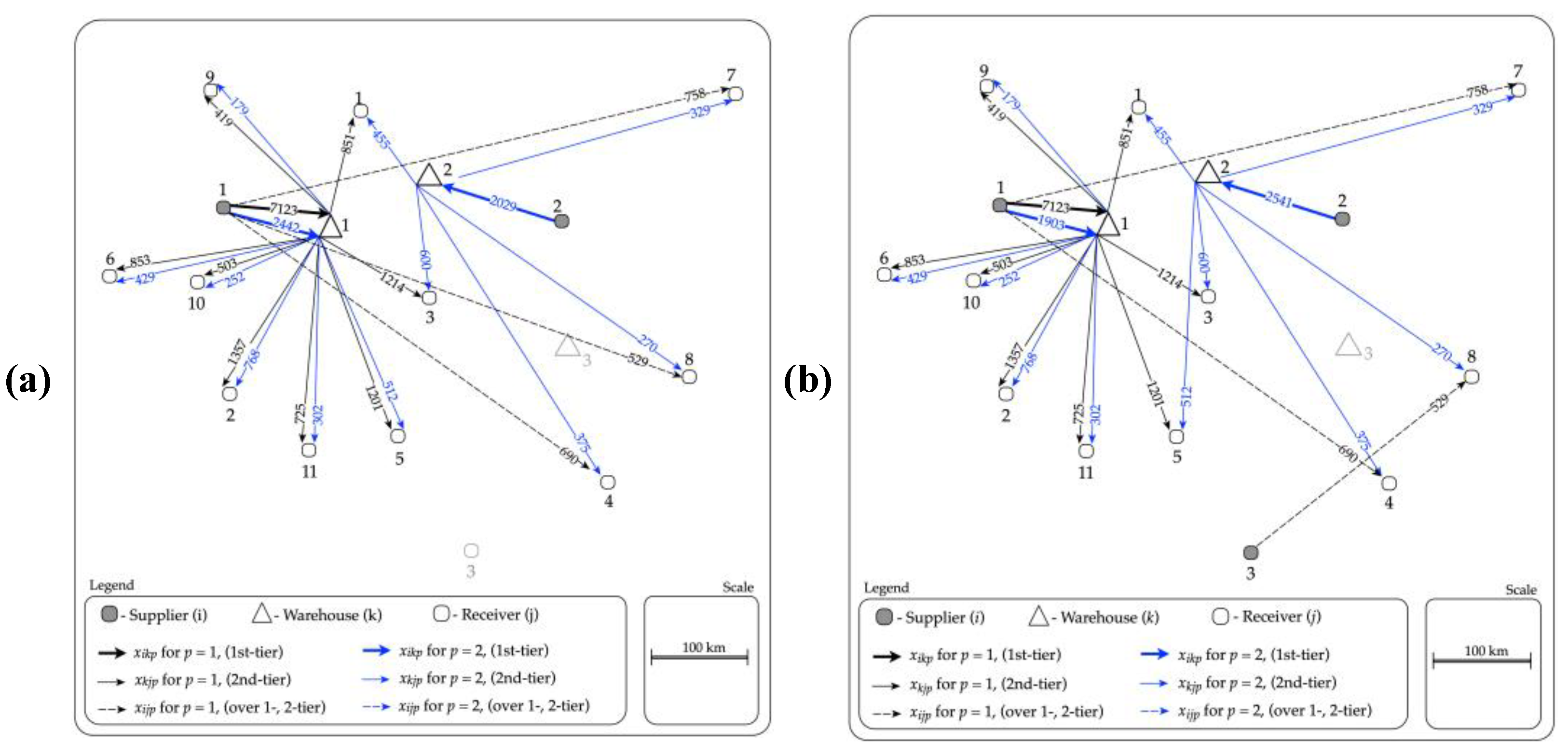
• The deliveries within p = 1 to recipient j = 8 (529 packs) are performed from supplier i = 1 (S1) or supplier i = 3 (S2);
• The deliveries within p = 2 to recipient j = 5 (512 packs) are performed from warehouse k = 1 (S1) or warehouse k = 2 (S2);
• The volume of deliveries from supplier i = 1 to depot k = 1 within p = 2 differs substantially, i.e., 2442 (packs) in S1 and 1903 (packs) in S2, and from supplier i = 2 to depot k = 2 is 2029 in S1 and 2541 in S2.

The values of the objective functions and their components, including (T^SD, T^DR, T^SR, W^D,f, and W^D,v) for an omni-channel distribution system are presented in

Table 3. Optimisation results: omni-channel vs. multi-channel distribution system.

Component of Objective Function	Unit	Omni-Channels				Multi-Channels
		S1		S2		S1		S2
		p = 1	p = 2	p = 1	p = 2	p = 1	p = 2	p = 1	p = 2
		qikp > 0	qikp > 500	qikp > 10	qikp > 500	qikp > 0	qikp > 500	qikp > 10	qikp > 500
		qikp ≤ 10	qikp ≤ 727	qikp ≤ 25	qikp ≤ 727	qikp ≤ 10	qikp ≤ 727	qikp ≤ 25	qikp ≤ 727
TSD	k.PLN/mth	0.899	42,528	2248	42,900	0	41,760	0	42,528
TDR	k.PLN/mth	27,907	78,988	69,767	80,152	0	79,509	0	78,988
TSR	k.PLN/mth	31,988	0	48,061	0	147,238	0	221,221	0
T	k.PLN/mth	60,794	121,516	120,076	123,052	147,238	121,269	221,221	121,516
WD,v	k.PLN/mth	64,107	150,398	64,107	148,862	0	153,563	0	150,398
WD,f	k.PLN/mth	2520	16,200	2520	16,200	0	16,200	0	16,200
W	k.PLN/mth	66,627	166,598	66,627	165,062	0	169,763	0	166,598
T + W	k.PLN/mth	127,421	288,114	186,703	288,114	147,238	291,032	221,221	288,114
		415,535		474,817		438,270		509,335
Savings	%	5.2		6.8		0		0

. The contrast of the final result, i.e., T + W value, is evident. It equals 59.3 k (PLN/mth), which is the difference between 474.8 k (PLN/mth) in S2 and 415.5 k (PLN/mth) in S1.

To compare this result with the reference solution, the authors optimised the structure of the multi-channel distribution system, which is dedicated to serve two commercial channels separately. The product flow between p = 1 and p = 2 is forbidden, i.e., r_ikp, r_kjp, and r_ijp equal 1. Using the previously mentioned parameters, the optimal multi-channel distribution system was achieved. Its graphic representation for S1 and S2 is presented in Figure 4c,d, respectively. The objective function of this distribution system is presented in Table 3.

In that case, two out of three alternative suppliers (i = 1 and i = 2) take part in the distribution process. Similarly, recipient alternative depot locations are applied to (k = 1 and k = 2). This structure guarantees that all deliveries within p = 1 (100% volume) are preformed directly from supplier i = 1 to recipients, and within p = 2, all deliveries (100% volume) are carried out from suppliers via depots. Since the result of optimisation multi-channel distribution system was set as a reference point in the experiments, one can compare an equivalent result of S1 and S2 for omni-channel vs. multi-channel options of distribution system, see Table 3. Based on the value of objective function T + W, it is noted that the omni-channel solution is favoured with respect to the multi-channel. The difference in T + W between these solutions is about 5 to 8%. The greater difference in favour of an omni-channel solution is noticeable when comparing the S2 scenario, i.e., the use of a larger weight range for unit load size used within p = 1, i.e., q_ijp = (10.1, 25.0) kg.

3.4. Sensitivity Analysis

A sensitivity analysis was carried out regarding the key parameters of the optimization model, including the storage and transport operations, as well as the demand fluctuation. The aim of this analysis was to determine which of the parameters and to what extent they affect the configuration of the omni-channel distribution network. To maintain the consistency of the analysis, a uniform relative range of variability of the considered parameters was determined, ranging from 0.5 to 1.5 (with 0.1 gradation) of the original value of each parameter applied to the optimization procedure. As a result, changes were observed in the objective function and its components (T, W). The changes in configuration of a distribution network within commercial channel was analysed along with the share and its role in the channels. All the observed trends were supposed to lead to more generic phenomena than the specific decision problem. The absolute values of the considered parameters applied to the optimisation model are presented in

Table 4. Variability ranges of the analysed parameters of the optimisation model.

Indices		Parameters
p	k	cijp(qijp)		cikp(lik)	ckjp(lkj)	$h_{kp}^f$	$h_{kp}^v$	Djp
-	-	PLN/pack	PLN/EUR	PLN/vkm	PLN/vkm	PLN/mth	PLN/pack	pack/mth	EUR/mth
1	1					1260–3780	4.5–13.5	(209, 678)–(628, 2035)	-
1	2	(16.18, 24.31)	-	(1.5–4.5)	(0.75–2.25)	1075–3225	6.0–18.0
1	3					1205–3615	8.5–25.5
2	1					4350–13,050	17.5–52.5	-	(89, 384)–(268, 1152)
2	2	-	(52.5–157.5)	(1.5–4.5)	(1.5–4.5)	3750–11,250	16.0–48.0
2	3					4600–13,800	22.5–67.5

.

The first part of the sensitivity analysis was carried out with reference to demand changes, applied to p = 1 (see Figure 5a,c) and p = 2 (see Figure 5b,d), and taking into account the different load size for p = 1, i.e., (0.1, 10.0) kg, see Figure 5a,b, and (10.1, 25.0) kg, see Figure 5c,d.

The analysis proved that a relatively wide range of demand variability results in the following phenomena:

• It does not change the number of warehouse facilities of each p-channel; one facility for p = 1, i.e., k = 1 in Figure 5a,c, and two facilities for p = 2, i.e., k = 1 ∧ k = 2, see Figure 5b,d;
• The changed demand applied to one channel does not change the number of facilities in another channel;
• It does lead to significant changes in the load volume structure; for channel p = 2, the volume structure per facility is 100% across k = 1 for (0.5, 0.7) D_jp and 55% across k = 1 and 45% across k = 2 for (0.7; 1.4) D_jp, see Figure 5b,d;
• The scale of volume structure change is more noticeable, the load unit is larger ((pack) for p = 1 vs. (EUR) for p = 2), and as a result, the increase in W components becomes more progressive referred to T, see Figure 5b,d vs. Figure 5a,c.

Another part of the analysis concerns the evaluation of the impact of transport cost changes per unit on the structure of the omni-channel distribution network. This analysis was performed with respect to transport tariffs dependent on the load weight per unit, i.e., c(q) and transportation distance c(l). In this paper, the first type of analysis is presented as it is more valuable for the purpose of the research.

The variation analysis of transport cost per unit, depending on the unit of load weight c(q), was performed with reference to both channels, i.e., p = 1, see Figure 6a,c, and p = 2, see Figure 6b,d, and to the different load size for p = 1, i.e., q_ikp = (0.1, 10.0) kg, see Figure 6a,b, and q_ikp = (10.1, 25.0) kg, see Figure 6c,d. The achieved results prove that the relatively wide range of variability of the transport cost depending on the size of freight, and independent of the distance, causes the following phenomena:

• A certain interval of c_ijp(q_ijp) changes stimulates the changes in the number of warehouse for individual sale channels; for interval (0.5, 0.8), c_ijp(q_ijp) all deliveries to j-recipients at p = 1 are carried out directly, i.e., the warehouse facilities are omitted, and for interval (0.8, 1.5) c_ijp(q_ijp), from one to three facilities are applied to, see Figure 6a,c;
• The change in transport cost per unit applied to one channel does not affect the change of the number of facilities in another channel;
• Specific intervals of c(q) lead to significant load volume structure changes (for p = 1 and q_ikp = (0.1, 10.0) kg load volume across k = 1 varies from 0 to 100%, see Figure 6a, and for q_ikp = (10.1; 25.0) kg load volume across k = 1 is 0–88%, 0–10% for k = 2, and 0–13% for k = 3, see Figure 6b; for p = 2 and interval (0.5, 0.8) c_ijp(q_ijp), the load volume across k = 1 and k = 2 varies from 0 to 80%, while for interval (0.8, 1.5), c_ijp(q_ijp) remains unchanged.

The changes in transport cost per unit applied to one channel have a limited effect on the volume structure within another channel (some changes applied to p = 1 have an impact on the volume structure for p = 2 in the wide spectrum of the analysis, see Figure 6a,c, while changes applied to p = 2 do not cause changes in the volume structure for p = 1, see Figure 6b,d).

The last part of the sensitivity analysis deals with the evaluation of an influence of unit storage cost changes on the structure of the omni-channel distribution network. This analysis can be performed with reference to both fixed and variable unit storage costs, however, due to the insignificant impact of fixed storage cost changes, the further deep analysis is limited to results on variable costs (see Figure 7), exclusively. This part of the analysis has been performed in the same cross-sections as before.

As far as obtained results are concerned, it has been proven that variable unit storage cost changes result in the following phenomena:

• In a very narrow range of $h_{{}_{kp}}^v$ changes, for a relatively very low value of $h_{{}_{kp}}^v$ changes, it influences the number of warehouse facilities for each channel of distribution network configuration, i.e., for p = 1 and q_ikp = (10.1, 25.0) (kg), two facilities exist (k = 1 ∧ k = 3), see Figure 7c; for p = 2 and the range (0.5, 0.6) $h_{kp}^v$, three facilities exist vs. two facilities for the remaining range of $h_{{}_{kp}}^v$ (k = 1 ∧ k = 2), see Figure 7b,d;
• Changes in the variable warehousing cost per unit applied to one channel does not affect the changes in the number of facilities in another channel;
• It leads to significant changes in the volume structure (for p = 1 and q_ikp = (0.1, 10.0) (kg), the volume across single facility k = 1 varies from 0 to 100% for a narrow range of $h_{{}_{kp}}^v$ changes, i.e., (1.0, 1.4), see Figure 7a; for p = 1, and q_ikp = (10.1, 25.0) (kg) for individual facilities it ranges from 0 to 30%, see Figure 7c for k = 1 ∧ k = 3, but for p = 2, a significant change in volume structure occurs (from 0 to 57%) for (0.5; 0.8) $h_{{}_{kp}}^v$);
• Changes applied to one channel have a limited impact on the volume structure in another one, i.e., changes introduced within p = 1 are translated into a very narrow range of the volume structure changes for p = 2 (from 0 to 12% of total volume); some changes applied to p = 2 do not reflect in the changes of volume structure for p = 1; see Figure 7b,d.

4. Conclusions

4.1. Result of the Research

The result of this research proves both the correctness of the optimisation model as well as the legitimacy of holistic optimizing of a distribution system in an omni-channel distribution system. The correctness of the proposed optimization model was confirmed on the basis of computational experiments. The values of decision variables were assessed with respect to the legitimacy of product flow at the first and the second tier of the distribution system. The validity of the holistic optimisation was demonstrated by way of comparing the results of the optimisation of distribution system for an omni-channel distribution system with reference to the optimisation of distribution system for each channel separately (multi-channel option).

The computational experiments performed in this research, although in fact related to the simplified case, render it possible to determine the estimated benefits of the omni-channel vs. the multi-channel distribution systems. The essence of the work was not to conduct an analysis of computational efficiency of optimising a complex, i.e., large-sized, decision problem but to identify potential benefits of designing an omni-channel solution. Depending on the applied parcel load and the adequate tariffs, a holistic optimization results in 5–8% savings on objective function (transportation and storage costs), compared to its competitor.

A configuration of the omni-channel distribution system was carried out based on the sensitivity analysis, referred to the key parameters of the optimization model, including warehouse and transport policy, as well as the level of demand. The applied changes were within a relatively wide range of variability, covering from 50% of the reduction to 50% of the increase in their primary values. As a result, it was discovered which of these parameters, and to what extent, influenced reconfiguration of the omni-channel distribution system. The observations made in such a context can help formulate some general principles regarding the configuration of the two-tier omni-channel distribution system, as follows:

• A significant change in the demand level with reference to one of the commercial channels does not result in a change in the number of facilities essential within the distribution system responsible for servicing this channel; it leads, however, to significant change in the structure of the product flow via these facilities.
• A change in the value of such parameters as the load unit index (dependent on distance) or the variable storage index, in relation to one of the commercial channels, causes a change in such quantities as the number of facilities and the structure of the flow of goods through the individual facilities of the considered part of the distribution system.
• Changes in the values of individual parameters of the optimisation model in relation to the distribution system responsible for servicing one of the commercial channels do not affect the change in the number of facilities responsible for servicing the other commercial channels; however, they significantly affect the structure of the product flow through these facilities.

Based on the conducted research, it is possible to formulate several practical guidelines supporting managerial decisions in the field of omni-channel distribution network design. The most important observations and suggestions referred to this case can be formulated as follows:

• The use of the omni-channel concept allows achieving noticeable benefits in contrast to multi-channel solutions; in the analysed case, 5–8% of operating costs savings is reached.
• The change in the structure of product flow through individual facilities in the distribution network depends mainly on the variation of such parameters as demand, transport rate, depending on the load size, and variable storage cost. The greatest sensitivity occurs, however, while changing the transport cost per unit c(q). In a relatively narrow range of the cost variation, it may lead to the disappearance of the product flow through the facility, or this flow can increase up to 100% of the total volume.
• The changes of all analysed parameters in relation to one of the commercial channels do not result in a change in the facilities serving other commercial channels.
• The number of facilities in the structure of the distribution network to a large extent depends on the variation of transport cost per unit c(q); the influence of the storage cost variations on the number of facilities is not significant, and this number does not depend on the demand variation, which, in fact, is crucial in the models with an unlimited capacity of facilities.

4.2. Limitation of the Research

The results of the research presented in this paper fill the identified research gap and contribute to the development of knowledge in the optimization of omni-channel distribution networks design area. However, there are identified the following limitations in practical application:

• The degree of complexity of the considered omni-channel distribution network structure is low, i.e., the analysed network is two-tiered, including senders, depots, and recipients.
• The degree of computational complexity of a distribution network expressed by the number of objects at each tier is low; the computations are performed for a relatively small instance, and in the case of a higher complexity, it is necessary to apply approximate procedures to search for a near-optimal solution in an acceptable computation time CPU.
• The transport functions are simplified to the shortest path in a direct one-to-one relation; the proposed model does not consider a typical one-to-many routing problem; it is, however, an acceptable simplification while a typical strategic decision problem is considered, including the distribution network design problem.

4.3. Further Research

Further research in the field of the optimisation of omni-channel distribution systems will be considered with respect to both economic and methodological aspects. From the economic point of view, an analysis of various forms of tariffs used by parcel carriers will be analysed. As a result, some observation of the impact of these parameters on the design and configuration of distribution systems are expected. From the methodological point of view, the research is expected to extend the optimisation model, to examine several further logistics issues, including the following:

• Diversified parcel structure, i.e., diversified weight ranges;
• Feet composition, i.e., variable structure of the means of transport used;
• Variable vehicle utilisation, i.e., introducing a variable degree of vehicle capacity utilisation;
• Do-or-buy, i.e., different structure of transport and warehouse service performed by own resources or the outsourced logistics contractors;
• Frequency of deliveries, i.e., the implementation of fixed vs. variable delivery schedule.

From the methodological point of view, it is also necessary to consider what impact the introduction of several evaluation criteria, including economic, technical, environmental, and social aspects, will have on the structure of the omni-channel distribution system under consideration.

References

1. Biggs, C.; Suhren, J. Omnichannel Alchemy: Turning Online Grocery Sales to Gold, The Boston Consulting Group Report, 1–20. 2013. Available online: https://www.bcg.com/publications/2013/retail-growth-omnichannel-alchemy-online-grocery-sales (accessed on 21 November 2018).
2. Hübner, A.; Holzapfel, A.; Kuhn, H. Distribution systems in omni-channel retailing. Bus. Res. 2016, 9, 255–296. [Google Scholar] [CrossRef] [Green Version]
3. Beck, N.; Rygl, D. Categorization of multiple channel retailing in multi-, cross-, and omni- channel retailing for retailers and retailing. J. Retail. Consum. Serv. 2015, 27, 170–178. [Google Scholar] [CrossRef]
4. Yadav, V.S.; Tripathi, S.; Singh, A.R. Exploring omnichannel and network design in omni environment. Cogent Eng. 2017, 4, 1382026. [Google Scholar] [CrossRef]
5. Chopra, S. How omni-channel can be the future of retailing. Decision 2016, 43, 135–144. [Google Scholar] [CrossRef]
6. Brynjolfsson, E.; HU, Y.J.; Rahman, M.S. Competing in the Age of Omnichannel Retailing. MIT Sloan Manag. Rev. 2013, 54, 23–29. [Google Scholar]
7. Abdulkader, M.M.S.; Gajpal, Y.; ElMekkawy, T.Y. Vehicle routing problem in omni-channel retailing distribution systems. Int. J. Prod. Econ. 2018, 196, 43–55. [Google Scholar] [CrossRef]
8. Geoffrion, A.M.; Graves, G.W. Multicommodity distribution system design by Benders decomposition. Manag. Sci. 1974, 20, 822–844. [Google Scholar] [CrossRef]
9. Geoffrion, A.M.; Graves, G.W.; Lee, S.J. A management support system for distribution planning. INFOR 1982, 20, 287–314. [Google Scholar] [CrossRef] [Green Version]
10. Gelders, L.F.; Pintelon, L.M.; van Wassenhove, L.N. A location-allocation problem in a large Belgian brewery. Eur. J. Oper. Res. 1987, 28, 196–206. [Google Scholar] [CrossRef]
11. Klose, A.; Drexl, A. Facility location models for distribution system design. Eur. J. Oper. Res. 2005, 162, 4–29. [Google Scholar] [CrossRef] [Green Version]
12. Laport, G.; Nickel, S.; Saldanha da Gama, F. Location Science; Springer: Berlin/Heidelberg, Germany, 2015. [Google Scholar] [CrossRef]
13. Melo, M.T.; Nickel, S.; Saldanha-da-Gama, F. Facility location and supply chain management—A review. Eur. J. Oper. Res. 2009, 196, 401–412. [Google Scholar] [CrossRef]
14. Farahani, R.Z.; Rezapour, S.; Drezner, T.; Fallah, S. Competitive supply chain network design: An overview of classifications, models, solution techniques and applications. Omega 2014, 45, 92–118. [Google Scholar] [CrossRef]
15. Mangiaracina, R.; Song, G.; Perego, A. Distribution network design: A literature review and a research agenda. Int. J. Phys. Distrib. Logist. Manag. 2015, 45, 506–531. [Google Scholar] [CrossRef]
16. Swaminathan, J.M.; Tayur, S.R. Models for supply chain in e-business. Manag. Sci. 2003, 49, 1387–1406. [Google Scholar] [CrossRef] [Green Version]
17. Ishfaq, R.; Defee, C.C.; Gibson, B.J.; Raja, U. Realignment of the physical distribution process in omni-channel fulfilment. Int. J. Phys. Distrib. Logist. Manag. 2016, 46, 543–561. [Google Scholar] [CrossRef]
18. Alptekinoğlu, A.; Tang, C.S. A model for analysing multi-channel distribution systems. Eur. J. Oper. Res. 2005, 163, 802–824. [Google Scholar] [CrossRef]
19. Xie, W.; Jiang, Z.; Zhao, Y.; Hong, J. Capacity planning and allocation with multi-channel distribution. Int. J. Prod. Econ. 2014, 147, 108–116. [Google Scholar] [CrossRef]
20. Zhang, S.; Lee, C.K.M.; Wu, K.; Choy, K.L. Multiobjective optimization for sustainable supply chain network design considering multiple distribution channels. Expert Syst. Appl. 2016, 65, 87–99. [Google Scholar] [CrossRef]
21. Lim, S.F.W.T.; Srai, J.S. Examining the anatomy of last-mile distribution in e-commerce omnichannel retailing: A supply network configuration approach. Int. J. Oper. Prod. Manag. 2018, 38, 1735–1764. [Google Scholar] [CrossRef] [Green Version]
22. Raza, S.A.; Govindaluri, S.M. Omni-channel retailing in supply chains: A systematic literature review. Benchmarking Int. J. 2021, 28. [Google Scholar] [CrossRef]
23. Ya-Jun, C.; Chris, K.Y.L. Omni-channel management in the new retailing era: A systematic review and future research agenda. Int. J. Prod. Econ. 2020, 229, 107729. [Google Scholar] [CrossRef]
24. Shpak, N.; Kyrylych, T.; Greblikaitė, J. Diversification models of sales activity for steady development of an enterprise. Sustainability 2016, 8, 393. [Google Scholar] [CrossRef] [Green Version]
25. Si, Z.; Heying, Z.; Xia, L.; Yan, W. Omni-Channel Product Distribution Network Design by Using the Improved Particle Swarm Optimization Algorithm. Discret. Dyn. Nat. Soc. 2019, 1520213. [Google Scholar] [CrossRef] [Green Version]
26. Guerrero-Lorente, J.; Gabor, A.G.; Ponce-Cueto, E. Omnichannel logistics network design with integrated customer preference for deliveries and returns. Comput. Ind. Eng. 2020, 144, 106433. [Google Scholar] [CrossRef]
27. Huang, J.; Shi, X. Solving the location problem of front distribution center for omni-channel retailing. Complex Intell. Syst. 2021, 7. [Google Scholar] [CrossRef]
Figure 1. Structure of the considered two-tier omni-channel distribution system.
Energies 14 07700 g001
Figure 2. Structure of the considered omni-channel two-tier distribution system, including the options of delivering (a) parcels within p = 1, (b) EUR pallets within p = 2.
Energies 14 07700 g002
Figure 3. The structure of an omni-channel two-tier distribution system.
Energies 14 07700 g003
Figure 4. Volumes flow at two-tier distribution network, including omni-channel distribution: (a) p = 1, qikp = (10.1, 25.0) kg, (b) p = 1, qikp = (0.1, 10.0) kg, and multi-channel distribution for: (c) p = 1, qikp = (10.1, 25.0) kg, (d) p = 1, qikp = (0.1, 10.0) kg.
Energies 14 07700 g004aEnergies 14 07700 g004b
Figure 5. Sensitivity analysis of omni-channel distribution network configuration with reference to demand changes: (a) p = 1, qikp = (0.1, 10.0) kg, (b) p = 2, qikp = (0.1, 10.0) kg, (c) p = 1, qikp = (10.1, 25.0) kg, (d) p = 2, qikp = (10.1, 25.0) kg.
Energies 14 07700 g005
Figure 6. Sensitivity analysis of omni-channel distribution network configuration with reference to the changes of transport cost per unit (a) p = 1, qikp = (0.1, 10.0) kg, (b) p = 2, qikp = (0.1, 10.0) kg, (c) p = 1, qikp = (10.1, 25.0) kg, (d) p = 2, qikp = (10.1; 25.0) kg.
Energies 14 07700 g006
Figure 7. Sensitivity analysis of variable storage cost changes per unit to the configuration of omni-channel distribution network (a) p = 1, qikp = (0.1, 10.0) kg, (b) p = 2, qikp = (0.1, 10.0) kg, (c) p = 1, qikp = (10.1, 25.0) kg, (d) p = 2, qikp = (10.1, 25.0) kg.
Energies 14 07700 g007aEnergies 14 07700 g007b