Experimental Analysis of GBM to Expand the Time Horizon of Irish Electricity Price Forecasts

Abstract

In response to the inherent challenges of generating cost-effective electricity consumption schedules for dynamic systems, this paper espouses the use of GBM or Gradient Boosting Machine-based models for electricity price forecasting. These models are applied to data streams from the Irish electricity market and achieve favorable results, relative to the current state-of-the-art. Presently, electricity prices are published 10 h in advance of the trade day of interest. Using the forecasting methodology outlined in this paper, an estimation of these prices can be made available one day in advance of the official price publication, thus extending the time available to plan electricity utilization from the grid to be as cost effectively as possible. Extreme Gradient Boosting Machine (XGBM) models achieved a Mean Absolute Error (MAE) of 9.93 for data from 30 September 2018 to 12 December 2019 which is an 11.4% improvement on the avant-garde. LGBM models achieve a MAE score 9.58 on more recent data: the full year of 2020.

1. Introduction

On 1 October 2018, the Integrated Single Electricity Market (I-SEM) went operational. It is now the enduring operational electricity market for both the Republic of Ireland and Northern Ireland [1]. EirGrid plc and SONI Ltd. respectively act as the Single Electricity Market Operator (SEMO) for the island of Ireland. This market structure was drafted to integrate the all-island electricity market with European electricity markets [2].

Observing SEMO market data from the first half of 2021, the energy prices reflect a record season in the European electricity markets and Ireland was no exception. During this period, the average electricity prices in the Irish SEMO SPOT market were around EUR 81/MWh with a deviation of approximately EUR 15/MWh. These values are relatively high figures for the usual price levels at that time of year, which in the previous two years fluctuated at around EUR 43/MWh. The German EPEX SPOT market disclosed prices from negative to almost EUR 100/MWh in the first half of 2021. A monthly average of EUR 74.08/MWh for June 2021 was the highest in the market since October 2008 [3].

In [4], Croonenbroeck et al. empirically demonstrate that inaccurate energy price forecasts have an impact on efficiency losses. While the I-SEM architecture offers day-ahead price data, more advanced forecasts are required to grant more protracted forecast time horizons to facilitate energy cost aware scheduling [5], optimal inter-connector operation, demand-side response, load shifting, maintenance scheduling, generation expansion planning, and bilateral contracting [6]. Additionally, disparate to load forecasting, electricity price forecasting is much more complex because of its unique characteristics, ambivalence in operation and the recondite bidding strategies of its market participants [7]. Furthermore, if they are to survive in the now deregulated and competing commercial environment, expanded short-term electricity price predictions are fundamental to the decision-making mechanisms of market participants [8]. Consequently, electricity price forecasting remains an arduous task and, together with the aforementioned, plays an essential element in balancing power generation and its consumption [9].The electricity price forecasting (EPF) is essential for decision-making mechanisms of market participants to sur-vive in the deregulated and competing commercial environment.

Rather than being based on speculation, in general, it is understood that electricity markets have quasi-deterministic principles. Hence, the desire to predict or estimate the price based on variables or features that can describe the outcome of the market [10]. Work by Lucas et al. [11] focused on the application of the Gradient Boosting Machine (GBM) algorithm to the balancing market.

To the author’s knowledge, GBM-based research has not been published for electricity price forecasting in the I-SEM. This paper presents an examination of gradient boosting algorithms to propagate further the prediction time horizon of day-ahead electricity price forecasts. In particular, the appropriateness of the GBM, the Extreme Gradient Boosting Machine (XGBM), and the Light GBM (LGBM) algorithms are investigated.

Section 2 offers an overview of the Irish electricity market and the framework used to benchmark this research. The data used, experiments undertaken, and evaluation procedures are presented in Section 3. Finally, the principal conclusions are summarized in Section 4. In comparison to the work by O’Leary et al. [6], it was found that XGBM reduces the MAE by 11.4%.

2. Literary Context and Background

2.1. I-SEM Electricity Market

The de novo grid power exchange hub in Ireland, I-SEM [12], offers a platform for the efficient trading of energy in a progressive wholesale market. The single electricity market operator (SEMO) auctions allow buyers to adopt a real-time pricing tariff structure, acquiring energy at fluctuating market rates [2]. As per Figure 1, each day, the Day-Ahead Market (DAM) within the I-SEM electricity market sees the release of 24 h spot prices representing the 24 trade periods for a particular trade day (D). Thus, at 13:00 (D-1) daily, the EUR/MWh prices for the D period operating from 23:00 to 23:00 is known (00:00 to 00:00 CET). The experimental analysis presented here aims to exceed the prediction horizon of 13:00 D-1, i.e., the time the day-ahead prices presently become known to market participants for a particular D of interest.

The focus of this research is to generate an ever-advanced day-ahead forecast of the DAM price schedule, which can effectively be used as a two-day-ahead price forecast. Thus, moving to double the unit price lead time available for market stakeholders for generating schedules, etc.

2.2. Research Benchmark

Due to the limited body of published literature centered around the wholesale electricity market in Ireland, the findings from this research were evaluated and benchmarked against the experimentation results presented in [6,13], respectively. In [13], using data from 2010 to 2011, 2015–2016, and 2016–2017 for comparison purposes, Lynch et al. developed a support vector machine (SVM) based model for the prediction of day-ahead electricity prices in the now obsolete Single Electricity Market (SEM) in Ireland—the SEM arrangement ended 30 September 2018. The constructed k-SVM-SVR ensemble model comprised the k-means, SVM, and Support Vector Regression (SVR) algorithm. The ensemble operates as follows: data are classified into clusters employing the k-means algorithm. An SVM classifier model is trained to discriminate between data of the K clusters. A separate SVR regression model is then trained on each cluster of data. Unseen incoming data is classified and fed into the relevant SVR regression model. Subsequently, whilst adopting the work presented in [13] as a barometer, O’Leary et al. in [6] detailed a comparison of deep learning and conventional machine learning methods for electricity price prediction in the current I-SEM arrangement. Contingent to the I-SEM exchange, the results of the 10 best performing models are presented in

Table 1. Excerpt of experimental results ^ⱡ by O’Leary et al. [6].

Algorithm/Model	MAE
K Nearest Neighbor (KNN)	11.21
Linear Regression	11.52
Random Forest	11.54
Lasso Regression	11.62
k-SVM-SVR [13]	11.97
Bayesian Ridge	12.48
Gated recurrent unit	13.00
Ridge regression	13.38
Decision Tree	13.44
Densely connect network	13.73

^ⱡ Data used: 30 September 2018 to 12 December 2019. All models employed an 80/10/10 training, validation, and testing split. As per [14], to ensure statistical significance, i.e., where analysis based upon the normal distribution is valid, MAE values are averaged over 30 instances.

based on available data at the time for the period 30 September 2018 to 12 December 2019.

It was found in [6] that deep learning models did not provide an improvement in the overall model performance while being slower to train. Densely connected, long short-term memory, gated recurrent unit, convolutional, and Capsule networks were all implemented. The Capsule networks in particular were found to be approximately three orders of magnitude slower than the KNN model. The non-neural network models used were Bayesian Ridge regression, Gaussian process, Random Forest, Decision Tree, extra tree, SVR, K-SVM-SVR, linear regression, Lasso regression, and ridge regression. The authors of [6] used a recursive single-step forecasting modeling methodology, i.e., the model produces a 24 h forecast by making 24 consecutive predictions, with each prediction being used to fill in missing feature data for the subsequent prediction.

To enable this research to serve as a point of reference for future efforts in this domain, performance indicators or regression error metrics including the Mean Absolute Error (MAE), the Mean Squared Error (MSE), the Root Mean Squared Error (RMSE), the Coefficient of Determination (𝑅²), and the Mean Absolute Percentage Error (MAPE) for 2019/20/21 data is included.

3. Data, Experiments, and Evaluation

3.1. Data

Domain literature suggest chronological index parameters, lagged variables, and data relating to seasonality as strong potential model inputs [15]. Additionally, exogenous variables such as generation capacity, load profiles, and ambient weather conditions have already been identified as suitable variables to explain electricity price dynamics [16,17]. The impact of external variables on the Irish day-ahead I-SEM spot prices are comprehensively investigated here by examining their correlations using the Pearson Correlation Coefficient (PCC). Variables tested include air temperature, wind speed, wind direction [18], oil prices (https://github.com/datasets/oil-prices [1], accessed on 1 May 2021), and natural gas prices (https://www.eia.gov/dnav/ng/hist/rngwhhdD.htm [2], accessed on 1 May 2021). The effects of wind speed are particularly pertinent due to the increasing proliferation of renewable energy generation. From 2010 to 2020, wind penetration has increased incrementally from 1.39 to 4.3 MW [19]. Today, wind generation accounts for approximately 36% of Ireland’s electricity demand [20]. The effect of the penetration of wind energy is highly dynamic as it adversely affects the stability of load frequency control (LFC) systems [21] but dampens the volatility of electricity prices [22].

This research also reviewed metrological parameters pertaining to principal geographical locations in Ireland along with daily oil and natural gas prices across the EU. Natural gas prices, as well as the wind speed, ambient temperature, and precipitation in all selected counties yielded favorable PCC values—c.f.

Table 2. Excerpt of model feature correlations *.

Feature	PCC Value
Windspeed Galway	0.315
Windspeed Cork	0.286
Daily Natural Gas Prices	0.259
Windspeed Dublin	0.237
Temperature Dublin	0.143
Temperature Cork	0.120
Temperature Galway	0.107
Daily Oil Prices	0.088

* Based on data 1 January 2019 to 12 December 2019.

. Feature engineering is an experimental process in Machine Learning (ML) that involves creating new artificial features using the existing raw data streams. Engineered features induce novelty and are proved to have a significant impact on performance of ML models [23].

As well as examining the suitability of Gradient Boosting algorithms in the domain of Irish electricity price forecasts, this research explores the application of elementary mathematical transformations and combinations thereof, including sum, mean, square, logarithm, and square root of the aforementioned independent variables to generate new predictor variables. Applying feature importance and ranking accordance to the Pearson’s score achieved, an excerpt of the results attained is presented in

Table 3. Excerpt of feature engineering correlations ^ⱡ.

Feature	PCC Value
Expanding Window Price	0.396
Windspeed-Mean	0.318
Windspeed-Mean Square Root	0.313
Windspeed-Mean Square	0.308
Windspeed-Mean Logarithm	0.299
Daily Natural Gas Price–Square Root	0.257
Day of the year	0.256
Hour	0.254

ⱡ Based on data 1 January 2019 to 12 December 2019.

. Similar to the rolling window technique, it can be observed that the application of the expanding window mean method [24] on historical spot prices yielded the leading PCC value.

3.2. Experiments

To validate the proposed solutions by scientific means, the following details the methodology of experiments employed:

▪

Initial data collection, integration, cleaning, and preparation.

▪

Data preparation: computing hourly lag features to advance the target variable 24 time-steps.

▪

Exploratory Data Analysis (EDA) [25].

▪

Feature importance and feature engineering.

▪

Feature selection.

▪

Imputing missing values using backfilling.

▪

Eliminating instances (matrix rows) where the target variable value is missing.

▪

Data splitting into training, validation, and test sets.

▪

Data pre-processing: scaling of numerical features.

▪

Model training, cross validation (cv) and, using the randomized search technique, hyperparameter tuning on selected feature lags and 24 target values for day-ahead prediction with an hourly resolution. This process used 80% of the available data, i.e., 277 days.

▪

Evaluation on test set (constituting 20% of total data instances for the period 1 January to 12 December 2019 that are chronologically consecutive, i.e., 69 days).

▪

Model training, cross validation (cv), and hyperparameter tuning on randomly sampled training data for the period 30 September 2018 to 12 December 2019. The training and validation process involved 394 days of data.

▪

Evaluation on test set constituting 10% of randomly sampled data instances for the period 30 September 2018–12 December 2019, i.e., 44 days.

▪

For data metrics, 30 iterations of the latter two steps are performed—an averaged thereof taken as the final score.

The models were implemented in Python 3 using the scikit-learn [26], XGBoost [27], and LightGBM [28] libraries. These Python packages are built on C libraries via Cython for more efficient execution times [26]. With 24 (hourly prices) values to predict, each model makes 24 predictions simultaneously. To achieve this, 24 separate model instances were created during model training, i.e., one for each hour of D + 1. Models and transformers such as scalers were only fitted to training data to prevent leakage (experimental code/dataset is available upon request).

3.3. Evaluation

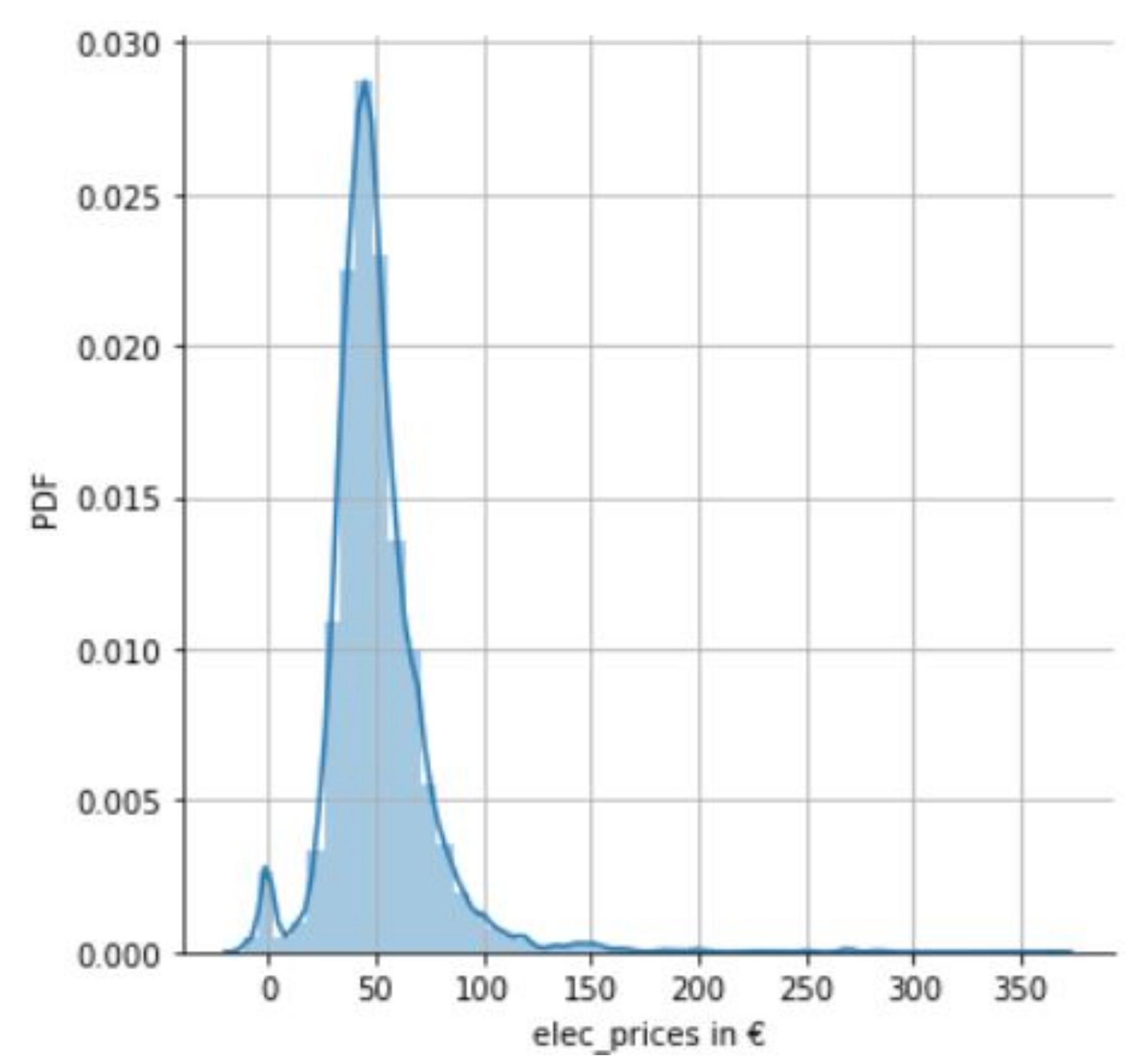
To demonstrate the volatility of the dataset, a univariate analysis of the electricity prices was performed for the evaluation period of interest, 1 January–12 December 2019. This saw min/max values of-EUR 11.86 and EUR 365, respectively. Figure 2 illustrates a Probability Density Function (PDF) of electricity prices for the same period, which indicates a higher than usual mean of circa EUR 50, as discussed earlier in the paper.

From the best features determined, detailed in part in Section 3.1, the Taguchi method, a process/product optimization method that is based on planning, conducting, and evaluating results of matrix experiments [29], was then employed to test the impact of each of the selected features and their impact on GBM, XGBM, and LGBM model performance for multi-step ahead prediction.

The tuned GBM based models were then evaluated on test sets comprising various permutations of the advocated input data streams. Combinations included the amalgamation of engineered and time-based features—an extract of the leading results of which are presented in

Table 4. MAE scores of best performing features–model combinations in each experiment for the period 1 January to 12 December 2019.

Features	Model	MAE Score
Basic time-based features + Wind Speed Average Logarithm	XGBM	10.045
Basic time-based features + Wind Speed Average Square root	XGBM	10.302
Basic time-based features + Wind Speed Average	XGBM	10.437
Basic time-based features + Wind Speed Average Square	XGBM	10.450
Basic time-based features + Wind Speed Galway	XGBM	10.493
Basic time-based features + Daily Natural Gas Price Square	LGBM	10.505
Basic time-based features + Windspeed Dublin	GBM	10.520
Basic time-based features + Daily Natural Gas Price	GBM	10.521
Basic time-based features + Daily Natural Gas Price Square Root	GBM	10.632
Basic time-based features + Wind Speed Cork	GBM	10.655
Basic time-based features + Expanding Window Price	LGBM	10.776
Basic time-based features	LGBM	10.788
Basic time-based features + Daily Natural Gas Price Logarithm	LGBM	11.073

. From this table, it is observed that a logarithm of the average wind speed as a feature had a significant impact on a model’s performance, deriving the lowest MAE score of 10.045. It was noted that including the logarithm of natural gas prices resulted in a weakened input matrix, producing one of the highest MAE values, 11.073.

To build on the results in Table 4, derived from following Taguchi’s method of experiments in assessing the various feature variables individually, the next effort explored an adjusted input matrix considering the top five features that augmented model performance. Statistical results from this, for two test periods, are presented in

Table 5. Summary of GBM, XGBM, and LGBM model performance ^♦ for the period 1 January to 12 December 2019.

Model	Metric	Score
GBM	MAE	10.79
	MSE	234.29
	RMSE	15.31
	MAPE	22.98
	R-Squared	0.10
XGBM	MAE	10.36
	MSE	218.42
	RMSE	14.78
	MAPE	22.07
	R-Squared	0.16
LGBM	MAE	10.68
	MSE	222.83
	RMSE	14.93
	MAPE	22.75
	R-Squared	0.12

^♦ all models used 23 lags of the top five features as per Table 2 and Table 3, respectively, and 24 lags of elec. prices.

and

Table 6. GBM, XGBM, and LGBM model performance ^♦ for the period 30 September 2018 to 12 December 2019.

Model	Metric	Avg. Score (30 Runs)
GBM	MAE	10.88
	MSE	285.23
	RMSE	16.78
	MAPE	19.84
	R-Squared	0.42
XGBM	MAE	10.021
	MSE	258.94
	RMSE	15.97
	MAPE	18.25
	R-Squared	0.48
LGBM	MAE	10.16
	MSE	261.10
	RMSE	16.06
	MAPE	18.51
	R-Squared	0.48

^♦ all models used 23 lags of top five features as per Table 2 and Table 3, respectively, and 24 lags of elec. prices. As per [14], to ensure statistical significance, MAE values are averaged over 30 instances.

, respectively.

In Table 5, which considers available 2019 calendar data for 1 January to 12 December, the minimum MAE score of 10.36 is achieved by the XGBM model. Additionally, observing the benchmark period, 30 September 2018 to 12 December 2019, Table 6 again elects the XGBM model as the algorithm of choice—achieving a MAE score of 10.021 over 30 runs.

Finally, this research analyzed the performance of GBM based models that gave consideration to all observed feature data. These results are displayed in

Table 7. Summary of GBM, XGBM and LGBM model performance ^♠ for the period 1 January to 12 December 2019.

Model	Metric	Score
GBM	MAE	10.93
	MSE	233.90
	RMSE	15.29
	MAPE	23.29
	R-Squared	0.08
XGBM	MAE	10.15
	MSE	210.04
	RMSE	14.49
	MAPE	21.63
	R-Squared	0.19
LGBM	MAE	10.58
	MSE	219.49
	RMSE	14.82
	MAPE	22.54
	R-Squared	0.14

^♠ 23 lags of all features examined and 24 lags of electricity prices.

and

Table 8. GBM, XGBM, and LGBM model performance ^♠ for the period 30 September 2018 to 12 December 2019.

Model	Metric	Avg. Score (30 runs)
GBM	MAE	10.85
	MSE	287.78
	RMSE	16.87
	MAPE	19.78
	R-Squared	0.41
XGBM	MAE	9.93
	MSE	255.03
	RMSE	15.86
	MAPE	18.10
	R-Squared	0.48
LGBM	MAE	10.15
	MSE	260.76
	RMSE	16.04
	MAPE	18.50
	R-Squared	0.48

^♠ 23 lags of all features examined and 24 lags of electricity prices.

, respectively, for the two test periods.

Looking at the 2019 test period, Table 7 presents the XGBM model as having the lowest MAE score of 10.15. Then, observing the benchmark period used by O’Leary et al. [6], i.e., 30 September 2018 to 12 December 2019, Table 8 again endorses the XGBM model as the algorithm of choice—achieving a MAE score of 9.93 over 30 runs.

For the purpose of scientific rigor and transparency in this domain, i.e., the Irish market, the outlined experimental methodology was also performed on 2020 data. These results should facilitate benchmarking outcomes on multiple contextual levels. Furthermore, as an additional feature, Brent crude and West Texas Intermediate (WTI) oil prices from the US Energy Information Administration with a correlation score of 0.16 was included. Results from the consideration of all conventional time series and engineered features are registered in

Table 9. Summary of GBM, XGBM, and LGBM model performance for the period 1 January to 31 December 2020.

Model	Outlier Processing	MAE Score
GBM	Capping	10.29
	Removal	10.40
	None	10.34
XGBM	Capping	10.08
	Removal	10.38
	None	10.15
LGBM	Capping	9.58
	Removal	9.63
	None	9.61

.

Additionally, included in Table 9 are the results of additional experiments to evaluate the efficacy of outlier preprocessing. Two means of outlier preprocessing were tested, i.e., outlier removal and outlier imputation. Outliers were first identified as being outside of a set threshold. This threshold was assumed to be four standard deviations from the mean. Outliers were then either capped at the outlier threshold or removed entirely from the training data. Outliers occurring in the test data were left unaltered.

It can be seen that the LGBM algorithm now presents itself as model of choice—yielding a single digit degree of error of 9.58 for the MAE. While outlier removal resulted in a slightly worse MAE score, outlier capping did consistently improve model performance.

From the experiments conducted in the research of this paper, it can be noted that there are some minor shortcomings of this methodology. Firstly, using different feature set and preprocessing combinations requires the reinitialization and retraining of models. This is a time-consuming process and is compounded multiplicatively by the forecast horizon size, i.e., by a factor of 24. Furthermore, the simulation time is also increased by a factor of 30 as experiments are repeated to achieve stable model rankings and scores.

4. Conclusions

In this paper, it was demonstrated that external/exogenous features have a significant impact on the day-ahead electricity spot prices. Wind speeds in counties Galway, Cork, and Dublin are highly correlated with the spot prices. This explains the sudden fluctuations of prices with variability in wind speeds. The natural gas price also exhibits a high degree of correlation with the spot prices.

Feature engineering has resulted in the creation of features that positively impacted price forecasting accuracy. Engineered features including expanding window price, average wind speed across the counties, and the mathematical transformations of daily natural gas prices has significantly strong correlations with the spot prices.

All feature-model combinations except for the logarithm of natural gas achieved MAE scores less than the baseline GBM model with basic time-based features as inputs for the period 1 January 2019 to 12 December 2019.

Multiple avenues for future research are evident from this study. While the GBM-based models presented expand the price forecast horizon by one day, a longer-term forecast could be achieved by adjusting the size of the bank of models used during model training, i.e., instead of training 24 model instances for a 24 h forecast, 48 instances could be trained for a 48-h forecast, and so on. It would also be possible to apply the specified forecasting methodology to other time series channels in the I-SEM such as load demand and the intra-day-ahead markets, IDA1 and IDA2, respectively.

The XGBM models with the top five features and all considered features as inputs achieved the best MAE (averaged over 30 runs/iterations) scores of 10.02 and 9.93, respectively, on the test set for the period 30 September 2018 to 12 December 2019. In conclusion, the XGBM model delivers an improvement of 11.4% when compared to the MAE score achieved by the KNR model implemented by O’Leary et al. [6]. The difference in input features used was ignored for this comparison. The final 𝑅² value of 0.49 approximately indicates that 49% of the data is fit on the XGBM model. Higher 𝑅² values indicate better model performance. Experimental results for 2020 data are also reported; LGBM models achieve an MAE score of just 9.58.