Article

Decoupling Analysis of Greenhouse Gas Emissions from Economic Growth: A Case Study of Tunisia

1
ISAEG, University of Gafsa, Rue Houssine Ben Kaddour, Sidi Ahmed Zarroug, Gafsa 2112, Tunisia
2
EUR ELMI, University Côte d’Azur, 5 Rue du 22ème BCA, 06300 Nice, France
*
Author to whom correspondence should be addressed.
Energies 2021, 14(22), 7550; https://doi.org/10.3390/en14227550
Submission received: 16 September 2021 / Revised: 28 October 2021 / Accepted: 7 November 2021 / Published: 12 November 2021

Abstract

:
The study examined the impact of different factors on greenhouse gas (GHG) emissions, by applying the extended STIRPAT model and decoupling analysis for Tunisia for the period 1990–2018. Furthermore, the study utilizes Tapio decoupling model, and the Auto-Regressive Distributed Lag (ARDL) bounds test approach to examine the relationship between the variables of greenhouse gas (GHG) emissions, economic growth, energy consumption, urbanization, innovation, and trade openness. The findings validated an inverted U-shape relationship between GDP and GHG emissions. In addition, we find that the consumption of renewable energy contributes to the reduction of GHG emissions in the long run. The findings call authority for the adaption of the regulatory framework relating to energy management, energy efficiency and the development of renewable energies, as well as to initiate energy market reforms, implement mitigation strategies and encourage investments in clean energies.

1. Introduction

The global warming and climate change, which occurred due to the increase in greenhouse gas (GHG) emissions in recent years, are among the most discussed issues in the world. The Intergovernmental Panel on Climate Change (IPCC) [1] highlights the importance of carbon emissions in contributing to GHG emissions. IPCC [1] reports that 76.7% of greenhouse gas emissions consists of carbon emissions produced mainly by developing countries which aim to accelerate their growth and increase domestic production in order to obtain better economic conditions. Moreover, according to Olivier and Peters [2], between 1990 and 2018, emissions were increased by 67.4%. Over this period, the biggest contributors to this increase were China (+370%), India (+340%), and the Middle East and North Africa (+210%). In addition, GHG emissions are presented as the main cause of pollution in the Kyoto Protocol, and it is clearly revealed that the greatest effect among these gases is caused by carbon dioxide (CO2) emissions (Udara Willhelm Abeydeera et al. [3]. Therefore, it is extremely important that policymakers rely on research outcomes to understand the current situation of GHG emissions in developing countries, thereby enhancing energy self-reliance and develop future strategies to reduce carbon emissions. At this stage, the literature on the main determinants of GHG emissions is gaining importance. Many different findings are obtained using data from different countries or a group of countries, and mobilizing decoupling decomposition analysis, econometric methods or other methodologies have led to the lack of a fundamental consensus on this issue. On the contrary, various studies agree on the fact that economic development, energy consumption, urbanization, innovation or even trade openness are among the important determinants of GHG emissions. Thus, the relationship between environmental quality and economic and social development factors has been widely explained by the environmental Kuznets curve (EKC) hypothesis which emerged in the early 1990s. According to the EKC hypothesis, during the early stages of development, there will be an increase in environmental pollution due to the use of energy-intensive technologies where economic growth is the main objective, but after reaching a certain level of economic development, socially conscious actions will be taken regarding the environment, there will be an increase in demand for clean and environmentally friendly energy. It is assumed that environmental degradation is avoided by using clean technologies. Many other models, methods and indicators have been proposed to quantitatively evaluate the determinants of GHG emissions. For example, STIRPAT (STochastic Impacts by Regression on Population, Affluence, and Technology) model, which is based on the IPAT (Influence, Population, Affluence, and Technology) model initially proposed by Ehrlich and Holdren in 1971, has often been used to assess the nexus between consumption of natural resources and pollutant emission, including GHG emissions. This model has been extended to include other variables such as urbanization, innovation, foreign direct investment, trade openness, financial development, and others. Furthermore, Tapio decoupling model or Logarithmic Mean Divisia Index (LMDI) decomposition method were also used to assess the decoupling relationship between GHG footprint and economic growth, and the respective contribution of the factors affecting GHG footprint decomposition.
With this perspective, due to its position as a developing country, Tunisia has the characteristics of a country with high energy demand and consumes intense fossil fuels. In this respect, it can be stated that there are important steps to be taken in the context of climate change. In order to carry out necessary studies in this area, greenhouse gas emissions that cause global warming should be analyzed in detail.
Against this background, the objective and main innovations of this research are two-fold. First, to examine whether there is a decoupling between economic growth and GHG emissions in Tunisia, relying on Tapio decoupling model. Second, to analyze the determinants of GHG emissions and the validity of EKC hypothesis, using the extended STIRPAT model.
This paper consists of five parts and organized as follows: after the introduction follows the literature review. Section 3 presents data and methodology. Section 4 provides the empirical results and discussion. Last section discusses conclusions and policy implications.

2. Literature Review

There is a variety of studies that investigate the causal relationship between GHG emissions, economic development, energy consumption, urbanization, innovation or even trade openness. According to Mardani et al., [4], the frequency of scientific articles in this field increased from 1996 to 2010, and the number of articles published in 2010 increased to nine articles per year and continued with this increasing momentum until 2019. China leads the way in this field with a rate of 18.86%, followed by Malaysia (14.86%), Tunisia (12.57%), Pakistan (7.43%), Turkey (6.29%) and Korea 4%. The most traditional empirical methodologies for countries case studies are the Johansen [5] cointegration approach, the ARDL method developed by Pesaran and Shin [6], decoupling models, and decomposition methods. While the case studies with panel data and Granger-type causality, the cointegration approach of Pedroni [7] and the causality model formalized by Dumitrescu and Hurlin [8] are usually used.
First, the studies that relate GHG emissions and economic growth and urbanization are covered. Traditional theory considers a positive relationship between increased economic growth, the rate of urbanization and GHG emissions (mainly CO2). Therefore, considering the effect of economic growth on the environment, two approaches have been proposed. The first estimates the relationship between per capita income and various environmental indicators. The second approach uses instead an index that measures the toxic intensity of sectoral manufacturing production to reflect the quality of the environment (air and water pollutants, solid waste per capita, access to drinking water, and deforestation indicators). Most of these studies tend to find that there is an inverted U-shaped relationship between pollution and income. This relationship is compared to that identified by Kuznets [9] who rather associated economic development with income inequalities. Empirical results reveal that increasing economic development and urbanization, through misuse of resources, increases GHG emissions [10,11,12,13,14,15,16].
The increase in environmental degradation is more observed in developing countries, especially in Asia, where energy intensity and the level of urbanization are very high. Ahmed et al. [10] find that energy consumption increases environmental degradation while verifying the existence of an environmental Kuznets curve for five Asian economies, they also find that there is a unidirectional causal relationship between energy consumption and urbanization. Amin et al. [11] have employed STIRPAT model, panel cointegration and FMOLS techniques to explore the dynamic relationship between CO2 emissions, urbanization, trade openness and technological innovation based on panel data from 13 Asian countries over the period 1985–2019. Their results reveal the existence of a long-term relationship among the variables. The panel causality analysis indicates a bidirectional causality between urbanization and CO2 emissions, technology and CO2 emissions, trade and CO2 emissions, in the long run. Behera and Dash [12], when incorporating the energy consumption of fossil fuels instead of the consumption of primary energy, find that there is a cointegration relationship between the energy consumption of fuels, urbanization, and CO2 emissions. For countries like China, where the urbanization process grows in parallel with energy consumption, which causes an increase in CO2 emissions [17]. Ding and Li [13] also explain that economic development factors are the main drivers of regional carbon dioxide emissions, compared to factors of structural change, energy intensity and social transition. Moreover, Gao et al. [18] used the Tapio decoupling model, coupled with the LMDI model and the Cobb-Douglas production function, to analyze the decoupling status of provincial carbon emissions from economic growth in China. Their results echoes previous findings on the favorable impacts of renewable energy on emission reduction. Zhang et al. [19] applied the PLS approach and Tapio decoupling to analyze the decoupling status of economic growth from greenhouse gas emissions, and found that for CO2, CH4, and N2O, only N2O emission showed a significant decoupling trend, while CO2 and CH4 emissions showed a slow decoupling trend. Similar outcomes were found by Kirikkaleli [20]. In Malaysia, in addition to the fact that economic growth contributes to CO2 emissions, increasing energy consumption rises this intensity [14]. Talbi [16] conducted a study on the causality between economic growth, energy consumption, energy intensity of road transport, urbanization, and fuel rate on CO2 emissions in Tunisia and found strong evidence that economic growth and urbanization play a dominant role in increasing CO2 emissions. Results further confirmed the EKC hypothesis. In contrast, Raggad [15] points out that the urbanization process does not significantly influence the increase in CO2 emissions in high-income countries such as Saudi Arabia, urbanization has a negative and significant impact on carbon emissions, arguing that urban development does not it is an obstacle to improving environmental quality.
Secondly, the studies that relate GHG emissions and energy consumption are covered. Empirical evidence suggests that there is a positive relationship between energy consumption and GHG emissions. At global level, this relationship varies according to countries and regions. Acheampong [21] finds that energy consumption causes carbon emissions in the Middle East and North Africa, but carbon emissions are negative in Sub-Saharan Africa and the Caribbean-Latin America. In contrast to the general theory, some authors mention that the consumption of energy from renewable sources reduces GHG emissions. For example, in Tunisia, Cherni and Essaber Jouini [22] find that the consumption of renewable energy contributes to the reduction of emissions while also having a positive effect on long-term economic growth. This is line in with the finding of Anwar et al. [23] for a group of ASEAN countries; Chen et al. [24] for China; Ito [25] for panel data of 42 developing countries; Njoh [26] for Africa; Zoundi [27] for a panel of 25 countries. Cai, et al. [28] find that there is no cointegration between clean energy consumption and CO2 emissions in Canada, France, Italy, the United States, and the United Kingdom, while this cointegration exists in Germany and Japan when CO2 emissions they serve as dependent variables. In this line, Amri [29] and Ben Jebli and Ben Youssef [30] find that clean energies does not contribute to the reduction of CO2 emissions in the long term, for Algeria and North Africa countries respectively.
The third group of studies includes the empirical evidence that relates GHG emissions and innovation, some authors argue that according to the level of technology the GHG emissions can be negatively affected [11,31,32]. Amri [31] find that innovation has not enabled Tunisia to decrease the CO2 emissions. This result is consistent with that obtained by Amin et al. [11] for the case of Tunisia. Dauda et al. [32] examined the EKC with total factor productivity as the proxy for innovation for Mauritius, Egypt, and South Africa. The results validated an inverted U-shape relationship between innovation and CO2 emissions.
Another variable frequently used as a determinant of GHG emissions and discussed in the study is trade openness. In the literature, the positive or negative effects of trade openness on environmental indicators can be explained by three different effects: scale effect, composition effect, and technical effect [33,34]. The scale effect expresses the increase in the quantity of pollution with the liberalization of trade and the increase in economic activities [35]. The structural effect is explained by changes in the composition of production, as well as by the increase in production volumes and the resulting specialization. In this process, it becomes important whether countries will specialize in pollution-intensive production or in the production of products that take environmental factors into account. Specialization in pollution-intensive activities will lead to overexploitation of the country’s natural resources and increasing environmental damage resulting from the production of these products. Therefore, such trade will have negative effects on the environment [33]. However, this situation will be reversed in countries that produce environmentally friendly production. Likewise, other countries trading with these countries will produce according to this demand in the country in question, and the positive effect of production on the environment will extend to larger areas [36]. The technical effect, on the other hand, is driven by the increase in commercial activities alongside with the increase in per capita income, the demand for more environmentally friendly clean technologies increases and investors change their production structures [37]. There are many studies in the literature dealing with the relationship between trade openness and the environment [11,38,39,40,41]. The different results obtained from these studies increase the importance of examining this topic. In this respect, to examine the existence of a long-run relationship between economic growth and the environmental pollution level in context of Vietnam, Do and Dinh [38] apply a Vector Error Correction model. They show that energy consumption and trade openness negatively affect CO2 emissions. Also, Mahmood et al. [40] investigated the asymmetrical effects of trade openness on CO2 emissions and the environmental Kuznets curve (EKC) hypothesis in Tunisia during the period 1971–2014. They prove an asymmetrical effects of trade openness on CO2 emissions. The effects of increasing and decreasing trade openness are found to be positive and insignificant on CO2 emissions, respectively. In the case of European economies, Jamel and Maktouf [39] investigate the causal nexus between economic growth, CO2 emissions, financial development, and trade openness. Their empirical results indicate a bidirectional Granger causality between among trade openness and pollution.

3. Data and Methodology

3.1. Data

In this study, yearly data stretching between 1990 and 2018 were used to capture the effects of economic growth, energy consumption, urbanization, innovation, and trade openness on environmental degradation in Tunisia. The dependent variable is LGHG, which represents environmental pollution and are measured as GHG emissions per capita. The independent variables are LGDP and LTRADE, which are GDP and trade openness, stand for affluence and are measured as GDP per capita and the sum of exports and imports as a share of GDP respectively, LREC and LNREC, which are renewable and non-renewable energies consumption represent energy structure and are calculated as energy consumption per capita, LURB represents urbanization, which are measured as population density, and LINNOV stands for domestic innovation and technological capabilities, which is measured as patent applications filed by residents. The data for LGHG, LGDP, LURB, LINNOV and LTRADE were extracted from the World Bank Development Indicators (WDI) database, while the data for LREC and LNREC were gathered from the US Energy Information Administration (EIA) database. Moreover, to reduce skewness, we transformed all the data into their natural logarithm. Table 1 presents the data, their sources, and some descriptive statistics.

3.2. Theoretical Framework

Several of the studies dealing with decoupling pollutant gas emissions from economic growth and energy use try to estimate the determinants of emissions to the atmosphere of some type of GHG, by a country or a group of countries. For this purpose, and from a methodological perspective, it is possible to distinguish between index decomposition methods and econometric methods. Index decomposition methods indicate that environmental impact can be decomposed into a series of factors. On the other hand, econometric methods can be used to perform hypothesis tests. Among the decomposition methods it is worth highlighting the Tapio [42] decoupling model and IPAT identity.

3.2.1. Tapio Decoupling Model

Tapio [42] indicates that the decoupling of pollutant gas (PG) emissions from economic growth is defined as the ratio of the change rate of PG emissions (∆PG) to the change rate of GDP (∆GDP) in a given period from a base year t − 1 to a target year t. Concretely, the Tapio decoupling index is expressed by the following equation as an elasticity index (DI).
D I = ( P G t P G t 1 ) / P G t 1 ( G D P t G D P t 1 ) / G D P t 1 = Δ P G / P G t 1 Δ G D P / G D P t 1 = % Δ P G % Δ G D P
where DI is the decoupling index, PGt−1 and GDPt−1 represent lags of PG emissions and economic growth, respectively, while ∆PG and ∆GDP denote the variation in PG emissions and economic growth. %PG and %GDP represent the growth rates of PG and GDP, respectively, between the base year and the target year.
A preliminary analysis of Tapio decoupling model was carried out by De Bruyn [43] who distinguishes two possibilities of decoupling in a growing economy, such as weak decoupling and strong decoupling (ΔPG < 0). Later, Tapio [42] initially considered three states in the degree of decoupling: coupling, decoupling and negative decoupling. A refinement by Tapio [42] and Vehmas et al. [44], distinguish between eight decoupling statuses as shown in Table 2 and Figure 1.
According to Tapio [42], in order to avoid overinterpreting slight changes as significant, elasticity values close to one continue to be considered as a coupling state. In Table 2, elasticity values between 0.8 and 1.2 are defined as a coupling state. This means that the change rate of GHG emissions is approximately equal to economic growth. For the other elasticity values, it is defined as a state of decoupling or negative decoupling. For a value of DI < 0, strong decoupling or strong negative decoupling can occur. The desirable scenario is the first, since PG emissions decrease in the face of economic growth, while in the second case the opposite occurs, that is, PG emissions increase in the face of a decrease in the economy. For values of 0 < DI < 0.8, a weak decoupling (PG emissions and economic growth increase) or weak negative decoupling (PG emissions and economic growth decrease) can occur. In both cases, the rate of variation of economic growth is higher in absolute value. For values of DI > 1.2, the possible state is a recessive decoupling (PG emissions and economic growth decrease) or expansive negative decoupling (PG emissions and economic growth increase). In both cases, the change rate of economic growth is lower in absolute value.

3.2.2. IPAT Identity

This identity arises from the paper-based debate between the researchers Holdren and Ehrlich and Commoner in the 1970s [45,46] about the anthropogenic forces that influence environmental impact. The IPAT identity states that the environmental impact can be broken down into three factors: population, affluence (GDP per capita) and a technological factor. Once this identity has been defined, some versions have been generated from it. The best known are the IPBAT [47], which includes, in addition to the aforementioned factors, the behavior of people (behavior), and the ImPACT [48], which disaggregate the technology factor into two factors: energy consumption and technological improvement.
The main limitations of the IPAT identity is that the number of factors is limited and also the impact of the factors is proportional, and it is considered that all factors affect the environment to the same extent. In addition, it does not allow hypothesis testing. Due to these problems, the STIRPAT model arises, which is nothing more than the stochastic version of the IPAT identity [49]. This STIRPAT model no longer belongs to the decomposition methods but is included in the econometric methods.
The specification of the STIRPAT model is as follows:
I i = a P i b A i c T i d e i
where t denotes the year, e is the error term, a is the constant term, and b, c and d are the elasticities of environmental impacts with respect to P, A and T, respectively, to be estimated.
The current research follows the theoretical framework introduced by Lin et al. [50] and contributes to theory by expanding the STIRPAT model to analyze the determinants of GHG emissions of Tunisia. This study conceptualizes the economic growth (GDP per capita) and trade openness as indicators for affluence to examine their impacts on GHG emissions. Additionally, the STIRPAT equation was expanded by including the square of GDP to test the environmental Kuznets curve hypothesis, energy structure, urbanization, and technology level. Hence, the proposed model takes the following form:
L G H G t = α 0 + α 1 L G D P t + α 2 L G D P t 2 + α 3 L R E C t + α 4 L N R E C t + α 5 L U R B t + α 6 L I N N O V t + α 7 L T R A D E t + e t
where α 1 , , α 7 are the models’ coefficients to be estimated and et denotes the error term.

3.3. Econometric Methodology

The above econometric model was regressed through Auto-Regressive Distributed Lag (ARDL) bounds test approach introduced by Pesaran and Shin [6] and Pesaran et al. [51]. This approach of estimation, contrary to the other approaches possesses numerous merits. Indeed, it performs better irrespective of order of integration of variables and estimates both long as well as short run coefficients simultaneously. Accordingly, ARDL technique is deemed to be robust in outcomes for small sample size [51]. Considering Equation (3), we specify the ARDL model as follows:
Δ L G H G t = β 0 + β 1 L G H G t 1 + β 2 L G D P t 1 + β 3 L G D P t 1 2 + β 4 L R E C t 1 + β 5 L N R E C t 1 + β 6 L U R B t 1 + β 7 L I N N O V t 1 + β 8 L T R A D E t 1 + i = 1 p 1 δ 1 Δ L G H G t i + i = 0 p 2 δ 2 Δ L G D P t i + i = 0 p 3 δ 3 Δ L G D P t i 2 + i = 0 p 4 δ 4 Δ L R E C t i + i = 0 p 5 δ 5 Δ L N R E C t i + i = 0 p 6 δ 6 Δ L U R B t i + i = 0 p 7 δ 7 Δ L I N N O V t i + i = 0 p 8 δ 8 Δ L T R A D E t i + η t
where Δ is the first-order differential operator, η t epresents the white noise and p 1 , , p 8 are the optimal numbers of lag which are determined by Akaike information criterion (AIC).

3.3.1. Unit Root Tests

Before proceeding with the ARDL techniques, a unit root tests must be done, to verify the stationarity of the different time-series data and to determine the order of integration of each variable. One way to do this is to use the traditional tests of augmented Dickey Fuller (ADF) [52] and Phillips and Perron (PP) [53] to test for the stationarity properties of the variables. Table 3 reports the results of these two tests. From this table, ADF test indicates that the null hypothesis of the unit roots cannot be rejected in level. These results strongly suggest that the variables in level are non-stationary and stationary in first-differences I(1). Similar results are obtained by the PP test except for LURB which is stationary at level I(0).

3.3.2. Lag Length for the ARDL Model

After finding the order of integration of the variables, the study needs to check the appropriate lag length for the different variables before the ARDL approach of cointegration. The model with the lowest available lag length selection criteria statistic is the optimal one. Considering AIC criteria, the ARDL (1, 1, 1, 2, 2, 2, 1, 1) model was identified to be the most appropriate.

3.3.3. Diagnostic and Stability Analysis

For the reliability and validity of the research findings, tests for residual heteroscedasticity, serial correlation, model misspecification and residual normality are conducted on the estimated model. The heteroscedasticity test selected is Breusch-Pagan-Godfrey. Breusch-Godfrey LM test was applied to check the serial correlation, while the Jarque-Bera statistic was used to test for normality. Ramsey RESET was performed to detect for both omitted variables and inappropriate functional form and to ensure that the model is correctly specified. The results of the diagnostic tests presented in Table 4 suggest that the findings of our study are robust and consistent.

4. Results and Discussion

4.1. Decoupling Index

Table 5 presents the trend of the decoupling states between the emissions of polluting gases (CO2 and GHG) and the economic growth obtained from the analysis of the Tapio elasticity analysis defined in Equation (1). The evaluation of the decoupling index and the decoupling status of pollutant gas emissions and economic growth of Tunisia from 1990 to 2018 reveals that growth rate of pollutant gas emissions and economic growth are variable, although that the elasticity value for several years is negative, but in most years, it turns out to be positive. Therefore, the weak decoupling state appears the most frequently during the period of 1990–2018, which suggest that the change rate of pollutant gas is obviously smaller than economic growth. The decoupling states of GHG emissions from economic growth can be classified into three periods: 1990–2000, 2001–2009 and 2010–2018. Hence, if the expected strong decoupling state (for GHG emissions) appears during 1990, 1994, 2013 and 2016, implying that pollutant gas declines while economic growth increases, the weak decoupling has appeared nine times, accounting for 100% in the period of 2001–2009. Analysis of the period 2010 to 2018 revealed that four different decoupling states emerged during this period: expansive negative decoupling in 2010, 2014, 2015 et 2017, recessive decoupling (RD) in 2011, weak decoupling in 2012 and 2018, and strong decoupling in 2016. Furthermore, according to Figure 2, it appears that Tunisia experienced a sudden change in the direction of decoupling after 2011. More specifically, it was found that GHG emissions and economic growth evolve negatively in the same direction in 2011. However, in 2013 the GHG emissions decreases and economic rate increases. This is virtually the same scenario as for the period 2014–2016. These findings reflect the different patterns of Tunisian economic development during the sampling period. Thus, the relative decrease of the growth rate for GHG emissions compared to the rate of change in economic growth can be explained by the relatively good economic performance over the period 2001–2009 and the reforms undertaken in terms of technology, changes in economic structure, mix of energy sources and energy efficiency. In addition, the mixed results associated with decoupling status during the period 2010–2018 may be caused by the effects of the recovery after the world economic crisis in 2008 and the consequences of the political and social instability that Tunisia experienced after the events of 2011. Finally, it seems that structural adjustment programs, privatization policy and decrease state spending in the 1990s are the main reasons of the fluctuations of economic activity and GHG emissions, and accordingly of the decoupling status during this period.
As the Tapio [42] decoupling analysis only provides the decoupling state from an elasticity perspective, the results of an in-depth analysis of the determinants of the decoupling of GHG emissions from economic growth, based on an econometric methodology, will be presented in the next subsection.

4.2. ARDL Model

4.2.1. ARDL Bounds Test for Cointegration

Long-run cointegration was examined through ARDL bounds testing approach based on the F-statistic with a null hypothesis no cointegration. The estimated F-statistic of 14.787 is above the upper critical bound at 1% significance level, thus rejecting the null hypothesis of non-cointegration between the variables which implies the existence of long-run cointegration relationships amongst the variables in the model. The test results are provided in Table 6.

4.2.2. Short-Run and Long-Run Estimates

The short-run and long-run ARDL estimate results are depicted in Table 7. The coefficient of the error correction term (ECT), which expresses the speed of adjustment of disequilibrium correction to a long-term equilibrium state, is negative and significant (−0.7722) at the significance level of 1%. Specifically, the speed of adjustment of any disequilibrium towards a long-term equilibrium is that approximately 77.22% of the disequilibrium in GHG emissions is corrected each year. Overall, the short-run and long-run coefficients (elasticities) are significant for all the variables retained in the model; except for trade openness, which is only statistically significant in the long run. It can also be observed that, most of the long run estimated coefficients are in line with theoretical expectations. As from the long-run estimates of the ARDL bounds test results, the coefficient of LGDP, LNREC and LURB were statistically significant in influencing GHG emissions at 1% level of significance. Moreover, the coefficients of LINNOV and LTRADE are significantly positive at the 5% and 10% level of significance respectively, while LGDP2 and LREC are negatively significant at the 1% level. Accordingly, a 1% rise renewable energy consumption will decrease GHG emissions by 0.07% in the long run. While the coefficient of non-renewable energy consumption (LNREC) reveals that 1% increase in LNREC cause a 0.15% raises in GHG emissions in the long run. Thus, policymakers must continue to adapt the regulatory framework relating to energy management, energy efficiency and the development of renewable energies, as well as to initiate energy market reforms, implement mitigation strategies and encourage investments in clean energies. It can be seen in Table 7 that the coefficient of LINNOV was positive, which means that technological innovations don’t help economic growth decoupling from GHG emissions. More specifically, a 1% rise in innovation triggers an increase of GHG emissions by 0.02%. This may have been due to the weakness of oriented energy-saving and emission-reduction technologies research and development (R&D) programs, where R&D and innovation spending are generally used to promote economic growth foremost. The coefficients of urbanization are found to significantly contribute to GHG emissions rise of about 0.49%, which is in line and consistent with the finding of Amin et al. [11], Behera and Dash [12] and Ding and Li [13]. Similarly, our findings indicate that trade openness leads to environmental degradation as it has a positive long-run effect on GHG emissions. A 1% increase in trade openness will intensify GHG emission by 0.07%. This result is also consistent with the studies of Jamel and Maktouf [39] and Mahmood et al. [40].
Furthermore, our empirical results support the existence of the EKC hypothesis for GHG emissions in Tunisia over the period 1990–2018. Indeed, the long run coefficients of GDP per capita and GDP per capita squared of 29.7361 and −1.7711 respectively, implying that an inverted U shape is well obtained. These results are similar to those of Mahmood et al. [40]. Moreover, building on our results, we conclude that the current relationship between economic growth and GHG emissions is on the ascending part of the EKC curve and has not yet reached the turning point. That is, with the continuous development of Tunisian economy, GHG emissions could rise but it is expected to fall after a certain level of GDP per capita. The estimated long-run relationship between GHG, GDP and GDP2 can be expressed as follows:
L G H G t 1 = β 1 L G D P t + β 2 ( L G D P t ) 2 = 29.736 L G D P + ( 1.771 ) ( L G D P ) 2
To find the location of the turning point of EKC, we set the first derivative of Equation (5) equal to zero (with respect to LGDP) and solved for LGDP; this gives:
29.736 + 2 ( 1.771 ) ( L G D P ) = 0 ( L G D P ) * = 8.395 G D P * = 4424.887
The value 4424.887 USD corresponds to the GDP per capita required for the GHG to begin their downward trajectory. Beyond this level, any increase in GDP translates into a reduction in GHG emissions.

5. Conclusions and Policy Implications

The main objective of the present study is to examine the decoupling effect of economic growth on GHG emissions in the context of Tunisia between 1980 and 2018. Our contribution to the literature is to use the decomposition methods Tapio [42] decoupling model and extended STIRPAT model and Auto-Regressive Distributed Lag (ARDL) bounds test approach. Also, we incorporate the energy consumption, urbanization, innovation, and trade openness as interesting variables to study their relationship with per capita GHG emissions, and to verify the EKC hypothesis. The empirical findings provided evidence of the decoupling effect of economic growth on GHG emissions, on the one hand, and support the existence of the EKC hypothesis for GHG emissions on the other.
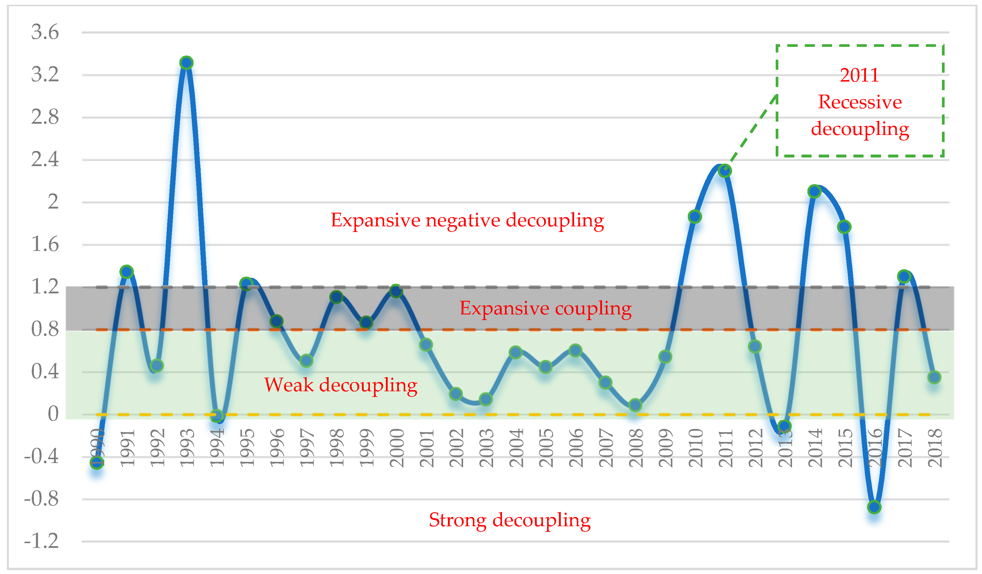
The decoupling analyses of economic growth on GHG emissions indicate that there are distinctive differences over the period 1990–2018. Between 2001 and 2009, Tunisian’s economic growth had been weakly decoupled from GHG emissions. For the years 1991, 1993, 1995, 2010, 2011, 2014, 2015, and 2017, Tunisia demonstrated expansive negative decoupling. Between 1998 and 2000 an expansive coupling occurred. For the periods 1990, 2013 and 2016, a strong decoupling was found.
After analyzing the decoupling elements, we found that urbanization, innovation, and non-renewable energies consumption effects was mostly responsible for the increase in GHG emissions. Also, our empirical results reveal that innovation contributes to the increase in GHG emissions in Tunisia, which seems to contradict theoretical predictions which consider innovation as one of the main channels for reducing greenhouse gas emissions. Such a result may provide proof that the Tunisian economy remains highly a consumer and still very little producer of technological innovations, particularly in the energy efficiency field. Public policies should balance technology-push, via subsidizing research and development and technology dissemination actions, and demand-pull policies for fostering innovations and accelerating their diffusion, through standards, taxes and cap-and-trade systems. Policy mixes may be more efficient than isolated measures. Hence, to strengthen the development of a low-GHG economy, Tunisia needs to rethink the urbanization structure and the energy management programs. Tunisia’s objective is to reach 30% of global electricity production from renewable energies by 2030. By having significant potential in wind and solar power, Tunisia has put in place a new regulatory framework through the promulgation of Law 2015–12 and its implementing government decree n° 2016–1123 of 24 August 2016 relating to the production of electricity from renewable energies. However, this sector faces several difficulties, and the installed energy capacity did not exceed 3% in 2019.
This work puts forward the following policy suggestions. Tunisia has relatively succeeded in establishing a legal regime favorable to the development of renewable energies. However, several obstacles hinder business owners from installing the equipment, real estate, and materials necessary to ensure the production of electricity from renewable energies. Indeed, the establishment of a project to build and operate an electricity production unit requires the intervention of several institutional and private actors. Entrepreneurs sometimes find it difficult to understand the authorization procedures for their projects. So, bureaucracy and the difficulty of accessing finance hamper the development of renewable energies. To remedy this shortcoming, the Tunisian Government must take certain measures: (1) involve private and civil society actors in carrying out any revision of the regulatory framework; (2) bring together the legal texts, application decrees and orders in a single collection to facilitate access and reading to potential investors; (3) clearly define responsibilities within institutions and strengthen human resources; and (4) involve local banks in the financing of renewable energies to promote investments in the field of renewable energies.

Author Contributions

Conceptualization, M.D.; methodology, M.D. and M.M.; formal analysis, M.D., M.M. and L.R.; writing—original draft preparation, M.D., M.M. and L.R.; writing—review and editing, M.D., M.M. and L.R. All authors have read and agreed to the published version of the manuscript.

Funding

This research received no external funding.

Institutional Review Board Statement

Not applicable.

Informed Consent Statement

Not applicable.

Data Availability Statement

The data that support the findings of this study are available from the corresponding author, upon reasonable request.

Conflicts of Interest

The authors declare no conflict of interest.

References

  1. IPCC. Global Warming of 1.5 °C; Masson-Delmotte, V., Zhai, P., Pörtner, H.-O., Roberts, D., Skea, J., Shukla, P.R., Pirani, A., Moufouma-Okia, W., Péan, C., Pidcock, R., et al., Eds.; An IPCC Special Report on the Impacts of Global Warming of 1.5 °C above Pre-Industrial Levels and Related Global Greenhouse Gas Emission Pathways, in the Context of Strengthening the Global Response to the Threat of Climate Change, Sustainable Development, and Efforts to Eradicate Poverty; IPCC: Geneva, Switzerland, 2019. [Google Scholar]
  2. Olivier, J.G.J.; Peters, J.A.H.W. Trends in Global CO2 and Total GHG Emissions; Report; PBL Netherlands Environmental Assessment Agency: The Hague, The Netherlands, 2019. [Google Scholar]
  3. Udara Willhelm Abeydeera, L.H.; Wadu Mesthrige, J.; Samarasinghalage, T.I. Global Research on Carbon Emissions: A Scientometric Review. Sustainability 2019, 11, 3972. [Google Scholar] [CrossRef] [Green Version]
  4. Mardani, A.; Streimikiene, D.; Cavallaro, F.; Loganathan, N.; Khoshnoudi, M. Carbon dioxide (CO2) emissions and economic growth: A systematic review of two decades of research from 1995 to 2017. Sci. Total Environ. 2019, 649, 31–49. [Google Scholar] [CrossRef] [PubMed]
  5. Johansen, S. Estimation and hypothesis testing of cointegration vectors in Gaussian vector autoregressive models. Econometrica 1991, 59, 1551–1580. [Google Scholar] [CrossRef]
  6. Pesaran, M.H.; Shin, Y. An Autoregressive Distributed lag Modelling Approach to Cointegration Analysis. In Econometrics and Economic Theory in the 20th Century: The Ragnar Frisch Centennial Symposium; Strom, S., Ed.; Cambridge University Press: Cambridge, UK, 1999; Chapter 11. [Google Scholar]
  7. Pedroni, P. Critical Values for Cointegration Tests in Heterogeneous Panels with Multiple Regressors. Oxf. Bull. Econ. And Stat. 1999, 61, 653–670. [Google Scholar] [CrossRef]
  8. Dumitrescu, E.-I.; Hurlin, C. Testing for Granger non-causality in heterogeneous panels. Econ. Model. 2012, 29, 1450–1460. [Google Scholar] [CrossRef] [Green Version]
  9. Kuznets, S. Economic growth and income inequality. Am. Econ. Rev. 1955, 45, 1–28. [Google Scholar]
  10. Ahmed, K.; Rehman, M.U.; Ozturk, I. What drives carbon dioxide emissions in the long-run? Evidence from selected South Asian Countries. Renew. Sustain. Energy Rev. 2017, 70, 1142–1153. [Google Scholar] [CrossRef] [Green Version]
  11. Amin, A.; Aziz, B.; Liu, X.-H. The relationship between urbanization, technology innovation, trade openness, and CO2 emissions: Evidence from a panel of Asian countries. Environ. Sci. Pollut. Res. Int. 2020, 27, 35349–35363. [Google Scholar] [CrossRef]
  12. Behera, S.R.; Dash, D.P. The effect of urbanization, energy consumption, and foreign direct investment on the carbon dioxide emission in the SSEA (South and Southeast Asian) region. Renew. Sustain. Energy Rev. 2017, 70, 96–106. [Google Scholar] [CrossRef]
  13. Ding, Y.; Li, F. Examining the effects of urbanization and industrialization on carbon dioxide emission: Evidence from China’s provincial regions. Energy 2017, 125, 533–542. [Google Scholar] [CrossRef]
  14. Etokakpan, M.; Solarin, S.A.; Yorucu, V.; Bekun, F.; Sarkodie, S.A. Modeling natural gas consumption, capital formation, globalization, CO2 emissions and economic growth nexus in Malaysia: Fresh evidence from combined cointegration and causality analysis. Energy Strategy Rev. 2020, 2017, 100526. [Google Scholar] [CrossRef]
  15. Raggad, B. Carbon dioxide emissions, economic growth, energy use, and urbanisation in Saudi Arabia: Evidence from the ARDL approach and impulse saturation break tests. Environ. Sci. Pollut. Res. 2018, 25, 14882–14898. [Google Scholar] [CrossRef] [PubMed]
  16. Talbi, B. CO2 emissions reduction in road transport sector in Tunisia. Renew. Sustain. Energy Rev. 2017, 69, 232–238. [Google Scholar] [CrossRef]
  17. Li, G.; Zakari, A.; Tawiah, V. Energy resource melioration and CO2 emissions in China and Nigeria: Efficiency and trade perspectives. Resour. Policy 2020, 68, 101769. [Google Scholar] [CrossRef]
  18. Gao, C.; Ge, H.; Lu, Y.; Wang, W.; Zhang, Y. Decoupling of provincial energy-related CO2 emissions from economic growth in China and its convergence from 1995 to 2017. J. Clean. Prod. 2021, 297, 126627. [Google Scholar] [CrossRef]
  19. Zhang, Z.; Ma, X.; Lian, X.; Guo, Y.; Song, Y.; Chang, B.; Luo, L. Research on the relationship between China’s greenhouse gas emissions and industrial structure and economic growth from the perspective of energy consumption. Environ. Sci. Pollut. Res. Int. 2020, 27, 41839–41855. [Google Scholar] [CrossRef]
  20. Kirikkaleli, D. New insights into an old issue: Exploring the nexus between economic growth and CO2 emissions in China. Environ. Sci. Pollut. Res. Int. 2020, 27, 40777–40786. [Google Scholar] [CrossRef]
  21. Acheampong, A.O. Economic growth, CO2 emissions and energy consumption: What causes what and where? Energy Econ. 2018, 74, 677–692. [Google Scholar] [CrossRef]
  22. Cherni, A.; Essaber Jouini, S. An ARDL approach to the CO2 emissions, renewable energy and economic growth nexus: Tunisian evidence. Int. J. Hydrogen Energy 2017, 42, 29056–29066. [Google Scholar] [CrossRef]
  23. Anwar, A.; Siddique, M.; Dogan, E.; Sharif, A. The moderating role of renewable and non-renewable energy in environment-income nexus for ASEAN countries: Evidence from Method of Moments Quantile Regression. Renew. Energy 2021, 164, 956–967. [Google Scholar] [CrossRef]
  24. Chen, Y.; Zhao, J.; Lai, Z.; Wang, Z.; Xia, H. Exploring the effects of economic growth, and renewable and non-renewable energy consumption on China’s CO2 emissions: Evidence from a regional panel analysis. Renew. Energy 2019, 140, 341–353. [Google Scholar] [CrossRef]
  25. Ito, K. CO2 emissions, renewable and non-renewable energy consumption, and economic growth: Evidence from panel data for developing countries. Int. Econ. 2017, 151, 1–6. [Google Scholar] [CrossRef]
  26. Njoh, A.J. Renewable energy as a determinant of inter-country differentials in CO2 emissions in Africa. Renew. Energy 2021, 172, 1225–1232. [Google Scholar] [CrossRef]
  27. Zoundi, Z. CO2 emissions, renewable energy and the Environmental Kuznets Curve, a panel cointegration approach. Renew. Sustain. Energy Rev. 2017, 72, 1067–1075. [Google Scholar] [CrossRef]
  28. Cai, Y.; Sam, C.Y.; Chang, T. Nexus between clean energy consumption, economic growth and CO2 emissions. J. Clean. Prod. 2018, 182, 1001–1011. [Google Scholar] [CrossRef]
  29. Amri, F. Carbon dioxide emissions, output, and energy consumption categories in Algeria. Environ. Sci. Pollut. Res. Int. 2017, 24, 14567–14578. [Google Scholar] [CrossRef]
  30. Ben Jebli, M.; Ben Youssef, S. The role of renewable energy and agriculture in reducing CO2 emissions: Evidence for North Africa countries. Ecol. Indic. 2017, 74, 295–301. [Google Scholar] [CrossRef] [Green Version]
  31. Amri, F. Carbon dioxide emissions, total factor productivity, ICT, trade, financial development, and energy consumption: Testing environmental Kuznets curve hypothesis for Tunisia. Environ. Sci. Pollut. Res. Int. 2018, 25, 33691–33701. [Google Scholar] [CrossRef] [PubMed]
  32. Dauda, L.; Long, X.; Mensah, C.N.; Salman, M.; Boamah, K.B.; Ampon-Wireko, S.; Courage, S.K.D. Innovation, trade openness and CO2 emissions in selected countries in Africa. J. Clean. Prod. 2021, 281, 125143. [Google Scholar] [CrossRef]
  33. Copeland, B.R.; Taylor, M.S. Trade, Growth, and the Environment. J. Econ. Lit. 2004, 42, 7–71. [Google Scholar] [CrossRef]
  34. Grossman, G.M.; Krueger, A.B. Environmental Impacts of a North American Free Trade Agreement. In The US-Mexico Free Trade Agreement; Garber, P., Ed.; MIT Press: Cambridge, MA, USA, 1993. [Google Scholar]
  35. Antweiler, W.; Copeland, B.R.; Taylor, M.S. Is Free Trade Good for the Environment? Am. Econ. Rev. 2001, 91, 877–908. [Google Scholar] [CrossRef] [Green Version]
  36. Brack, D. Balancing trade and the environment. Int. Aff. 1995, 71, 497–514. [Google Scholar] [CrossRef]
  37. Cole, M.A.; Elliott, R.J.R. Determining the trade–environment composition effect: The role of capital, labor and environmental regulations. J. Environ. Econ. Manag. 2003, 46, 363–383. [Google Scholar] [CrossRef]
  38. Do, T.; Dinh, H. Short-and long-term effects of GDP, energy consumption, FDI, and trade openness on CO2 emissions. Accounting 2020, 6, 365–372. [Google Scholar] [CrossRef]
  39. Jamel, L.; Maktouf, S. The nexus between economic growth, financial development, trade openness, and CO2 emissions in European countries. Cogent Econ. Financ. 2017, 2020, 1. [Google Scholar] [CrossRef]
  40. Mahmood, H.; Maalel, N.; Zarrad, O. Trade openness and CO2 emissions: Evidence from Tunisia. Sustainability 2019, 11, 3295. [Google Scholar] [CrossRef] [Green Version]
  41. Sebri, M.; Ben-Salha, O. On the causal dynamics between economic growth, renewable energy consumption, CO2 emissions and trade openness: Fresh evidence from BRICS countries Renew. Renew. Sustain. Energy Rev. 2014, 39, 14–23. [Google Scholar] [CrossRef] [Green Version]
  42. Tapio, P. Towards a theory of decoupling: Degrees of decoupling in the EU and the case of road traffic in Finland between 1970 and 2001. Transp. Policy 2005, 12, 137–151. [Google Scholar] [CrossRef] [Green Version]
  43. De Bruyn, S.M. Economic Growth and the Environment: An Empirical Analysis; Kluwer Academic Publishers: Dordrecht, The Netherlands, 2000. [Google Scholar]
  44. Vehmas, J.; Luukkanen, J.; Kaivo-oja, J. Linking analyses and environmental Kuznets curves for aggregated material flows in the EU. J. Clean. Prod. 2007, 15, 1662–1673. [Google Scholar] [CrossRef]
  45. Commoner, B. The Closing Circle: Nature, Man, and Technology; Jonathan Cape: London, UK, 1972. [Google Scholar]
  46. Ehrlich, P.R.; Holdren, J.P. Impact of population growth. Science 1971, 171, 1212–1217. [Google Scholar] [CrossRef]
  47. Schulze, P.C. I = PAT. Ecol. Econ. 2002, 40, 149–150. [Google Scholar] [CrossRef]
  48. Waggoner, P.E.; Ausubel, J.H. A framework for sustainability science: A renovated IPAT identity. Proc. Natl. Acad. Sci. USA 2002, 99, 7860–7865. [Google Scholar] [CrossRef] [PubMed] [Green Version]
  49. Dietz, T.; Rosa, E.A. Rethinking the environmental impacts of population, affluence, and technology. Hum. Ecol. Rev. 1994, 1, 277–300. [Google Scholar]
  50. Lin, S.; Wang, S.; Marinova, D.; Zhao, D.; Hong, J. Impacts of urbanization and real economic development on CO2 emissions in non-high income countries: Empirical research based on the extended STIRPAT model. J. Clean. Prod. 2017, 166, 952–966. [Google Scholar] [CrossRef]
  51. Pesaran, M.H.; Shin, Y.; Smith, R.J. Bounds Testing Approaches to the Analysis of Level Relationships. J. Appl. Econ. 2001, 16, 289–326. [Google Scholar] [CrossRef]
  52. Dickey, D.A.; Fuller, W.A. Likelihood Ratio Statistics for Autoregressive Time Series with a Unit Root. Econometrica 1981, 49, 1057–1072. [Google Scholar] [CrossRef]
  53. Phillips, P.C.B.; Perron, P. Testing for Unit Roots in Time Series Regression. Biometrika 1988, 75, 335–346. [Google Scholar] [CrossRef]
Figure 1. The schematic diagram of decoupling states.
Energies 14 07550 g001
Figure 2. Trend of decoupling effect of GHG footprint in Tunisia.
Energies 14 07550 g002
Table 1. Variables’ definition and Descriptive Statistics.
VariablesDescriptionObservationMeanStandard DeviationMinimumMaximumSource
LGHGGHG per capita: The ratio between greenhouse gas emissions and population (million metric tons of CO2 equivalent/person)293.1350.3822.4083.593WDI
LGDPGDP per capita: The ratio between gross domestic product (constant 2010 US$) and population293378.985766.3662224.8344408.334WDI
LRECThe ratio between energy consumption from renewables and population (Mtoe/person)290.0860.0350.0190.140EIA
LNRECThe ratio between total energy consumption (except renewables) and population (Mtoe/person)297.5601.6554.07810.216EIA
LURBPopulation density: (people per square km of land area)2964.4945.97053.05474.441WDI
LINNOVNumber of patent applications by residents2982.20758.50822.000235.000WDI
LTRADETrade openness: the sum of imports and exports normalized by GDP (% of the GDP)2990.78411.21276.655114.344WDI
Note: Variables are log-transformed.
Table 2. Criteria for Defining the Decoupling Status.
Decoupling Status%∆PG%∆GDPRange of DI
CouplingExpansive coupling (EC)>0>00.8 < DI < 1.2
Recessive coupling (RC)<0<00.8 < DI < 1.2
DecouplingWeak decoupling (WD)>0>00 < DI < 0.8
Strong decoupling (SD)<0>0DI < 0
Recessive decoupling (RD)<0<0DI > 1.2
Negative decouplingWeak negative decoupling (WND)<0<00 < DI < 0.8
Strong negative decoupling (SND)>0<0DI < 0
Expansive negative decoupling (END)>0>0DI > 1.2
Table 3. Results of Unit Root Tests.
VariablesLevelFirst-DifferenceOrder
Without TrendWith TrendWithout TrendWith Trend
LGHG−2.327−1.442−6.257 ***−6.987 ***I(1)
LGDP−1.723−0.078−4.168 ***−4.662 ***I(1)
LGDP2−1.849−0.017−4.137 ***−4.711 ***I(1)
LREC−1.669−1.575−5.579 ***−5.625 ***I(1)
LNREC−1.257−2.049−6.981 ***−7.118 ***I(1)
LURB−0.075−4.563 ***−5.187 ***−5.227 ***I(1)
LINNOV−0.384−3.655 **−6.591 ***−6.418 ***I(1)
LTRADE−1.230−4.077 **−5.850 ***−5.739 ***I(1)
LGHG−3.545−1.154−6.257 ***−7.833 ***I(1)
LGDP−1.665−0.171−4.168 ***−4.663 ***I(1)
LGDP2−1.789−0.017−4.137 ***−4.711 ***I(1)
LREC−1.661−1.529−5.611 ***−5.672 ***I(1)
LNREC−1.047−1.991−6.981 ***−7.207 ***I(1)
LURB−5.714 ***−5.828 ***−5.811 ***5.635 ***I(0)
LINNOV−0.754−3.706 **−17.081 ***−17.350 ***I(1)
LTRADE−0.843−3.258 *−6.773 ***−6.541 ***I(1)
Notes: The unit-root test was performed under the null hypothesis wherein the variables are homogeneous non-stationary. (***), (**) and (*) denote statistical significance level at 1%, 5% and 10%, respectively.
Table 4. Residual and Stability Diagnostics.
Diagnostic Statistics TestTest StatisticsProb.Result
Breusch-Pagan-Godfrey1.58860.2570No problem of heteroscedasticity
Breusch-Godfrey LM5.82130.1538No problem of serial correlations
Jarque-Bera3.39330.1833Estimated residual are normal
Ramsey RESET0.73700.4206Model is specified correctly
Table 5. Decoupling status of Tunisia’s economic growth.
YearPollutants GasYearPollutants GasYearPollutants Gas
CO2GHGCO2GHGCO2GHG
1990WDSD2000ECEC2010ENDEND
1991ENDEND2001ECWD2011RDRD
1992WDWD2002WDWD2012ECWD
1993ENDEND2003WDWD2013WDSD
1994WDSD2004WDWD2014ENDEND
1995ECEND2005WDWD2015ENDEND
1996WDEC2006WDWD2016SDSD
1997WDWD2007WDWD2017ENDEND
1998ECEC2008WDWD2018WDWD
1999ECEC2009WDWD
Source: Author’s own calculations.
Table 6. Results of ARDL Bounds Test.
Test StatisticValueSignificance.I(0) BoundI(1) Bound
F-statistic14.7871810%2.033.13
k75%2.323.5
2.5%2.63.84
1%2.964.26
Table 7. Estimated Short-run and Long-run Relationships.
VariablesCoefficientStd. Errort-StatisticProb.
Short-Run Coefficients
C−209.8684 ***40.1117−5.23210.0008
LGDP(−1)52.9062 ***9.80145.39780.0006
LGDP2(−1)−3.1518 ***0.5999−5.25250.0008
LREC(−1)−0.1296 ***0.0213−6.07630.0003
LNREC(−1)0.2739 ***0.06634.12940.0033
LURB(−1)2.6507 ***0.61694.29640.0026
LINNOV(−1)0.0437 **0.01762.48240.0380
LTRADE(−1)0.13930.08101.72020.1237
ΔLGDP25.0750 ***7.29943.43520.0089
ΔLGDP2−1.4863 ***0.4499−3.30310.0108
ΔLREC−0.0193 **0.0072−2.66460.0286
ΔLREC(−1)−0.0430 ***0.0110−3.91190.0045
ΔLNREC0.04540.03561.27610.2377
ΔLNREC(−1)−0.2172 ***0.0406−5.34590.0007
ΔLURB42.062 ***9.74194.31760.0026
ΔLURB(−1)62.0168 ***9.90336.26220.0002
ΔLINNOV0.0320 ***0.01063.01180.0168
ΔLTRADE−0.03490.0622−0.56200.5895
Long-Run Coefficients
LGDP29.7361 ***5.05515.88240.0004
LGDP2−1.7711 ***0.3114−5.68720.0005
LREC−0.0729 ***0.0097−7.49820.0001
LNREC0.1540 ***0.03124.93690.0011
LURB1.4899 ***0.29864.99010.0011
LINNOV0.0246 **0.00902.72520.0260
LTRADE0.0783 *0.04171.87700.0974
ECT−0.7792 ***0.1915−9.28880.0000
R-squared0.9886
Akaike info criterion−6.7470
Schwarz criterion−5.8351
Prob (F-statistic)0.0000 ***
Note: (***), (**) and (*) denote statistical significance level at 1%, 5% and 10%, respectively.
Publisher’s Note: MDPI stays neutral with regard to jurisdictional claims in published maps and institutional affiliations.

