Economic Model and Risk Analysis of Energy Investments Based on Cogeneration Systems and Renewable Energy Sources

Abstract

Today, distributed energy production is a key activity supporting energy systems in many countries around the world. Applicable regulations, fees and subsidies encourage entrepreneurs to look for solutions that will reduce operating costs and limit their negative impact on the natural environment. In the article, it was decided to carry out a technical and economic analysis and investment risk analysis for the distributed production of electricity and heat based on natural gas. Six scenarios were taken into account, depending on the number of gas engines, the use of the photovoltaic installation and the Organic Rankine Cycle (ORC) system. It has been shown that the most advantageous of the presented solution is the use of a system adjusted to the power of an industrial plant (return on investment in 4th year). The least beneficial for the investor are solutions aimed at the use and resale of energy supplemented with photovoltaic panels and an ORC system. An investment risk analysis and a sensitivity analysis were also performed. It shows how changes in electricity and gas prices and the environmental fee affect the profitability of investments. It has been shown that solutions with variable power are characterised by the lowest investment risk. The summary indicates the possible activities leading to greater economic efficiency. Such actions will be forced in the future by the market, political and environmental situation. Analyses such as these will allow entrepreneurs to thoroughly prepare for the European Union energy modernization process.

1. Introduction

In business, one of the major parameters influencing profitability is the price of energy. It depends on many variables such as fuel prices, environmental fees and exchange rates. Many of them can change with geopolitical conditions, which may gave a significant impact on the price of the final product and its competitiveness on market. The Emissions Trading System (ETS) market was introduced in 2005 and its main purpose is forcing modernisation of the energy sector in European Union. Now it is one of the main reasons for rising energy prices. It has a particular impact on the economy of countries where the energy sector is mostly based on hard coal and lignite. Depending on the type of energy produced, CO₂ emission factors for these fuels are among the highest and are within the range of 93 to 108 tCO₂/TJ [1]. Countries with the highest coal consumption are Germany, Poland and Turkey. The worst situation can be observed in Poland, where over 70% of energy is produced from this fuel [2]. A new energy strategy of Poland has been introduced in 2021. The main goals of modernisation of the national energy system are introducing nuclear energy, increasing the share of renewable energy sources, the transformation of heat energy systems and extending distributed energy [3]. For the last point, works over Baltic Pipe could increase imported natural gas in Poland. This could reduce the price of this fuel and have a positive effect on energy prices. Moreover, the CO₂ emission factor for methane is 55.8 tCO₂/TJ [1] and is almost half then for hard coal. Another method of reducing CO₂ emissions can be the use of alternative fuels such as ammonia, which can be produced using renewable energy sources [4]. Investigation shows that in a swirl burner it is possible to burn 5% of ammonia in fuel gases. The flameless technology improves this process by reducing the emission of nitrogen oxides by five times [5].

A good way to achieve mentioned above goals is to target distributed energy sources on the grids. Another argument for this solution is no ETS fees for energy producers with total power lower than 20 MW. Distributed energy is characterised by the use of smaller units of its production (electricity, heat, cold) in relation to conventional solutions. Often there are located in the area of their use. Thanks to this, it is possible to use low-temperature heat and the final efficiency of energy generation can be higher. In the case of conventional solutions, energy is lost during its transmission over long distances [6]. The most popular extended distributed energy are CHP units (Combine Heat and Power) mostly based on reciprocating engines. Analyses of this system in public buildings like hospitals or hotels were carried out [7,8,9]. The main parameter on which the nominal power of unit was focused was the minimum thermal power of the building. This allows the engine to work on nominal parameters and maximum efficiency for all the year. It also gives opportunity to get profits as high efficiently cogeneration certificates which could be sold. In the industry sector, the best condition for high-efficiency cogeneration could be found in thermal treatment companies. 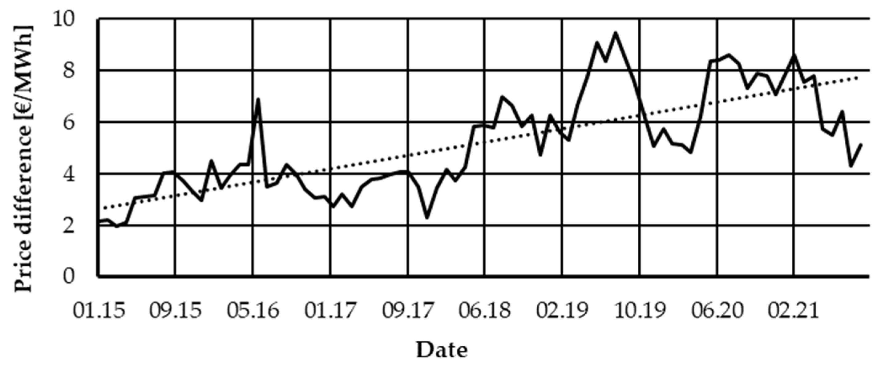An example of this is the paper industry where the demand for thermal power is similar all year [10,11]. Until now, in plants where thermal power has changed significantly, using CHP units were non-economic. The reason for this was the impossibility to achieve high-efficiency cogeneration and as result no certificate to obtain which allowed for the profitability of the investment. With current electricity prices, it may be necessary to use local cogeneration systems focused on electricity demand. This will cause high heat losses, but the growing ratio between the prices of electricity and natural gas shown in Figure 1 may be more important from an economic perspective for companies.

Another aspect suggesting using distributed energy production is its stability. Regions with problems of a power outage can still be found in Poland. However, it should be kept in mind that a significant part of these situations is caused by planned breaks, in most cases resulting from maintenance works on the power grid. The average value of outages over 2015–2020 was 413 MWh for 77 min. From these values, the value of unplanned outages was 94 MWh for 17 min [13]. For example, in Germany, which has one of the most reliable power grids in Europe, in 2015 there were 12 min and 42 s of power outages which was a consequence of extreme weather events. In Brazil, power cuts are more than 24 h a year, while in Japan it is 6 min a year. This result is caused by used energy microgrids. Every hour of power outage generates economic losses [14]. Simulations of four-hour power outages in Austria show a loss of 287 mln € [15]. This argument justified using the energy microgrid based at local power generator for example CHP units.

Searching for new sources of energy for existing industrial facilities requires the analysis of many variables to determine the profitability of the investment. Consider the daily and yearly energy consumption profile. It is also necessary to take into account the location of the buildings for renewable energy systems like photovoltaics (PV). Earlier works proved that analyses based on static economic models and risk economic models can be successfully used to assess investments in the modernisation of existing installations. Researchers from Slovenia proved that using models to assess investment risk can help decision-makers in making key decisions [16]. Usually in this type of analysis, the Monte Carlo Method (MCM) is used to estimate the behaviour of economic parameters which may help the decision, considering the risk in project sustainability. The examples of using MCM can be found in several works. The Edinaldo Jose da Silva Pereira research group analysed the energy generation systems with photovoltaic located on Amazon Region in Brazil. Their research, conducted by Monte Carlo Method (MCM), shows that considered installation are economically unviable without subsidies [17]. Arnold and Yildiz used the MCM approach to carry out a risk analysis based on an entire life-cycle representation of Renewable Energy Technology (RET) investment projects. They demonstrated that “Monte Carlo Simulation generates substantial value-added information with respect to project risk that is relevant for investors, lenders and the feasibility of project financing” [18]. Urbanucci and Testi used MCM to concern the implementation of a CHP system for a hospital. The analysed building is located in Italy. In conclusion, they say that “they have shown how traditional deterministic methods tend to oversize cogeneration units and overestimate cost savings” [19]. The Zaroni research group checked the economic risk of purchasing an electric generator to provide energy during peak time. Their research has shown that “diesel and natural gas-based generators can guarantee a low risk of return on investment to investors and such risk is truly dependent on the generator rated power” [20]. A good method to analyse risk in investments projects can be FMEA (Failure Mode and Effect Analysis) analysis but it is good only to consider one case so it will be impossible to use this method in this work. An example of using FMEA analysis to risk assessment is the risk analysis of geothermal power plants [21].

However, it should be remembered that the goal of all business activities in the market environment is the long-term economic well-being of business entities, which is determined by the profitability of the business [22]. For the company to make a profit, it is necessary to obtain financial indicators that suggest the success of the investment. The actions of entrepreneurs are not always clear. The Kliestik et al. research proves that the countries of the Visegrad group tend to manipulate earnings. Such distorted financial results, presenting an overly positive financial situation, may result in taking a risk that is inadequate to the current macroeconomic situation [23].

Based on the presented information it was decided to prepare a simulation model which allows one to estimate the payback time of energy investment for nowadays economic situation. The next part of the article presents a technical, economic and investment risk analysis for distributed production of electricity and heat based on natural gas. It was made for a model building located in the west-central part of Poland. Six variants of the power supply systems were created, starting from gas engines (GE) with constant and variable power. In the following variants, additional photovoltaic systems (PV) and Organic Rankine Cycle (ORC) were used.

2. Methods

To carry out the analysis, it was decided to choose an industrial plant located in Poland. Therefore, to obtain probable results, one should look at the situation in the energy market. Based on data from the Energy Regulatory Office, the electricity market is geographically divided, and the market has five large distribution network operators whose networks are directly connected to the transmission network [24]. They have a legal obligation to separate the distribution activities carried out by the system operator from other activities not related to electricity distribution (unbundling). In addition, in 2019, there were 184 enterprises designated as operators of distribution networks, operating as part of vertically integrated enterprises with no obligation to unbundle [24].

The price lists of the mentioned companies were used for further analysis. Based on the analysis of prices and trends, it was possible to estimate the current electricity price and its forecast value.

The analyses omitted: fixed costs of the company (building maintenance, leasing, etc.), costs of employee salaries, depreciation of equipment.

It was assumed that the planned investment would be covered with cash or external sources—therefore the costs related to the loan granted for the investment were not taken into account.

A reference system has been used to model facilities that were supplied in energy from the electricity grid and heating network. This system is commonly used for buildings located in cities. In comparison, six scenarios of the CHP system are connected with renewable energy installations.

2.1. Modernisation Setup

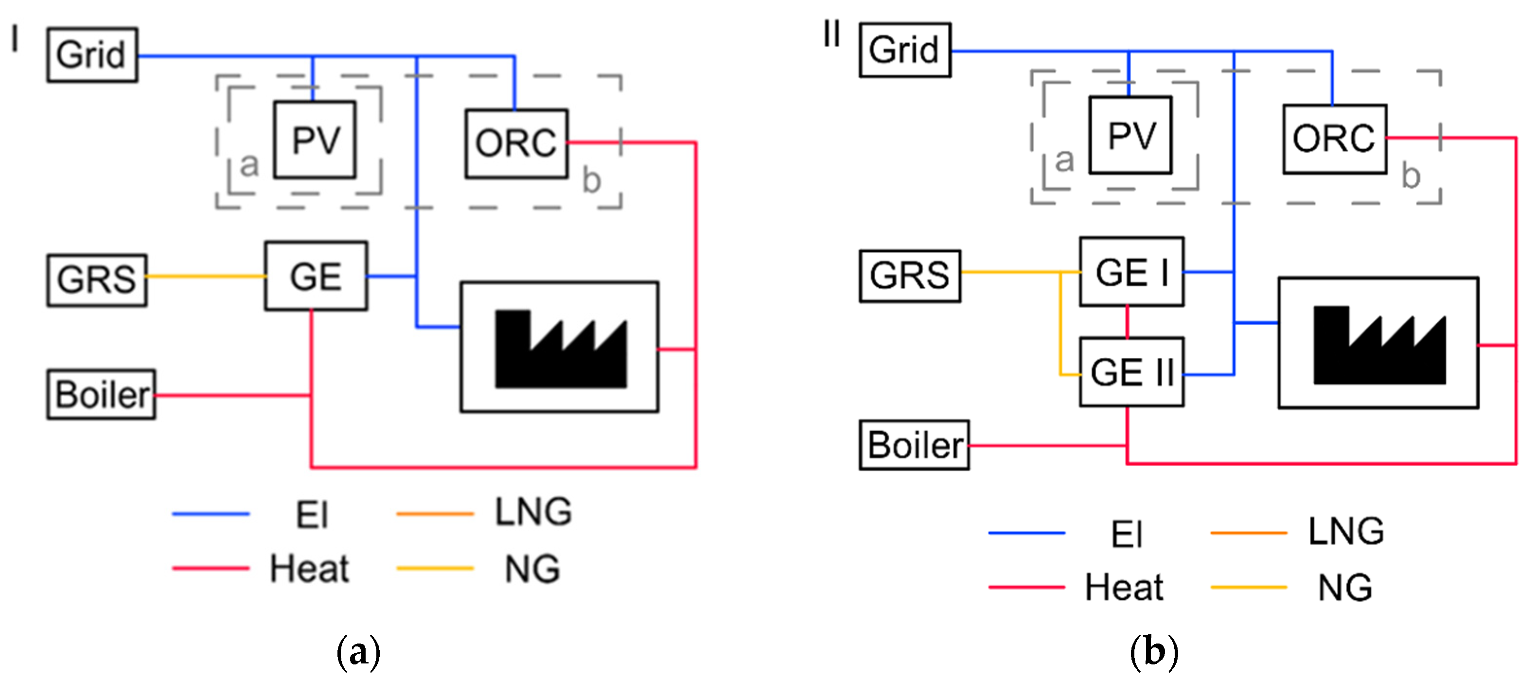
The first type of CHP systems (I) are based on the single gas engine which power cover the maximum electrical power demand of facilities. The power generator works on nominal power for all year the exception of service time. The difference between production and consumption of energy is sold to the electric grid. Waste heat from gas engines is used for heating buildings. In case of higher demands for heat, gas boilers were used.

In the second type of system (II), two gas engines with power 350 kWe and 650 kWe were used. The power of each engine was controlled by the actual hourly demand of facilities. According to load, it was assumed changes of mechanical and heating efficiency of CHP unit. Generated heat like in systems type I is used for heating buildings and in case of higher demand, assisted by gas boilers.

In presented systems, renewable energy system like photovoltaic (Ia, IIa) and ORC (Ib, IIb) were additionally implemented. Thanks to that waste heat could be also used to improve the overall efficiency of the CHP unit. The above system schemes were shown in Figure 2.

Analysis was prepared for existing facilities where electricity connection to the grid was left. It allows one to make maintenance of CHP units or its brake down without stops of production.

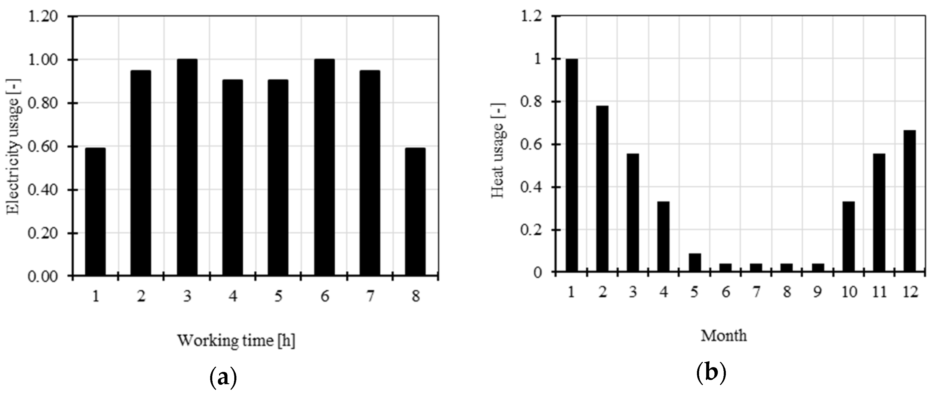
A shift system was used with a specific profile of relative electricity consumption shown in Figure 3. The building was located in the mid-west of Poland. Energy demand was determined based on average monthly temperatures and examples of buildings of this type. The values of the required power of the power connections are presented in

Table 1. Nominal power of energy connection.

Energy	Unit	Value
Electricity	kW	1000
Heat	kW	3500

.

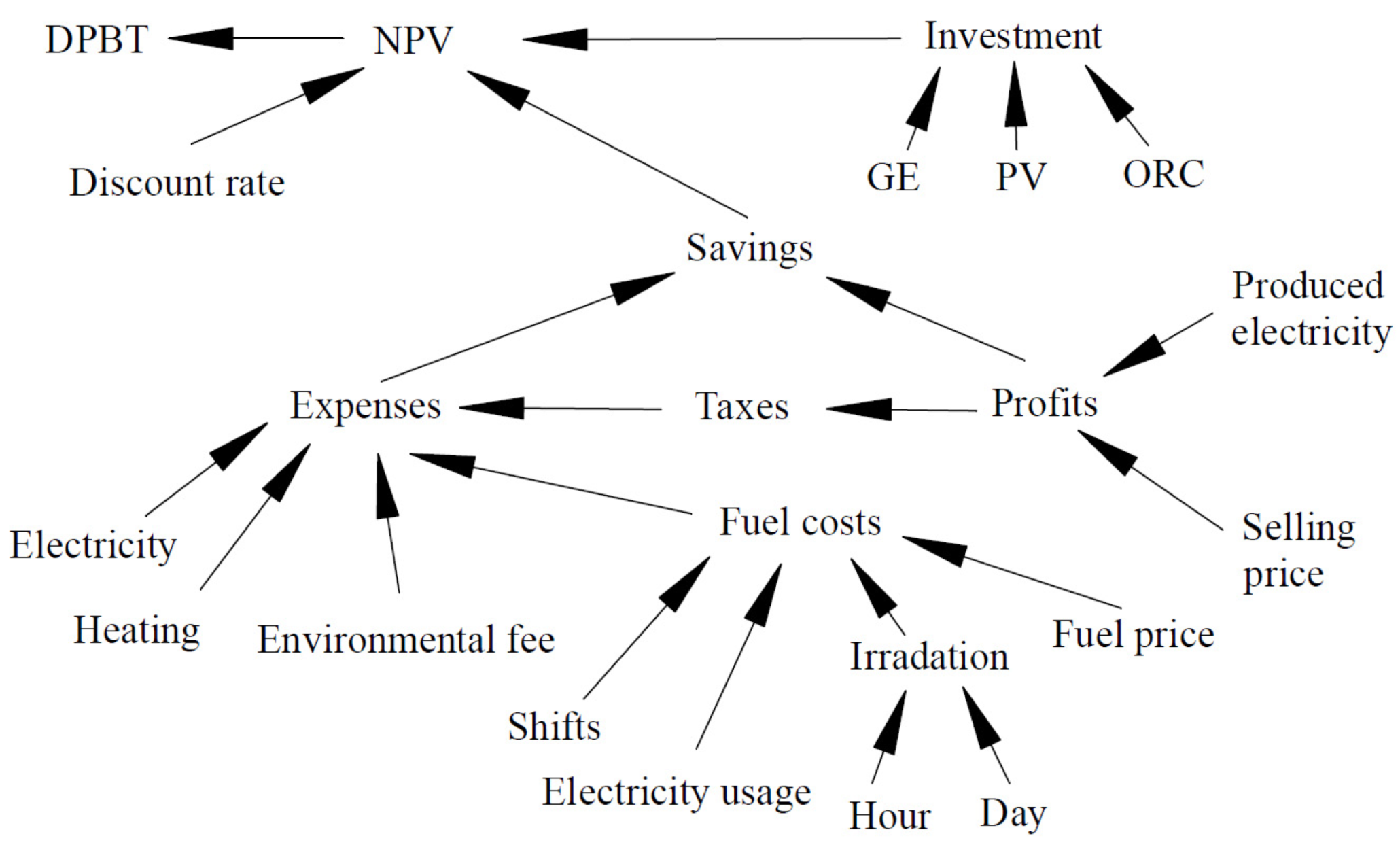
Figure 4 shows the graphic version of the model. The main elements influencing the Net Present Value (NPV) were: investment costs and the difference in annual costs to the reference system. These depend on the prices of electricity, gas and energy consumption. The last one depends on the day and the number of job shifts. All scenarios were prepared for three work shifts.

2.2. Irradiation Model

The model uses a variable value of energy generated from photovoltaic panels for systems Ia, Ib, IIa, IIb. The changes in the angle of incidence (AOI) of sunlight with respect to azimuth and zenith depending on the day and time were used for this. Installation of photovoltaic panels were fixed to the roof of the production halls without the possibility of tracking the position of the sun. For the obtained data, the AOI of sunlight on the panels was calculated depending on the day and time. The AOI angle was calculated using the Formula (1) [25]:

$$AOI=co{s}^{-1}\left[cos\left(\beta \right)·cos\left(\varphi \right)+sin\left(\beta \right)·sin\left(\varphi \right)·cos\left(\psi -\gamma \right)\right]$$

(1)

where $\beta$ is the angle of inclination of PV modules; $\varphi$ is the angle between the zenith and a line from the sun; $\psi$ is the angle from the north for a line from the sun and $\gamma$ is PV module azimuth angle from the north.

Based on the database [26], the distributions of sun irradiance during the day for individual months were adopted. The total solar radiation reaching the photovoltaic panels $E$ was calculated according to the Formula (2) [27]:

$$E=E_b+E_g+E_d=DNI·cos\left(AOI\right)+GHI·a·\frac{\left(1-cos\left(\beta \right)\right)}{2}+DHI$$

(2)

where $E_b$ is direct normal irradiance on PV panels, $E_g$ is global horizontal irradiance on PV panels, $E_d$ is diffuse horizontal irradiance on PV panels, $DNI$ is direct normal irradiance; $GHI$ is global horizontal irradiance; $DHI$ is diffuse horizontal irradiance, $a$ is ground Albedo coefficient and $\beta$ is the angle of inclination of PV modules.

Instantaneous power of PV system was calculated by Formula (3) where was taking account actual irradiation data, AOI angle and area of PV panels:

$$N_{PV}=A_{PV}E$$

(3)

where $A_{PV}$ is the area of PV panels, $E$ is the actual total solar irradiance on PV panels.

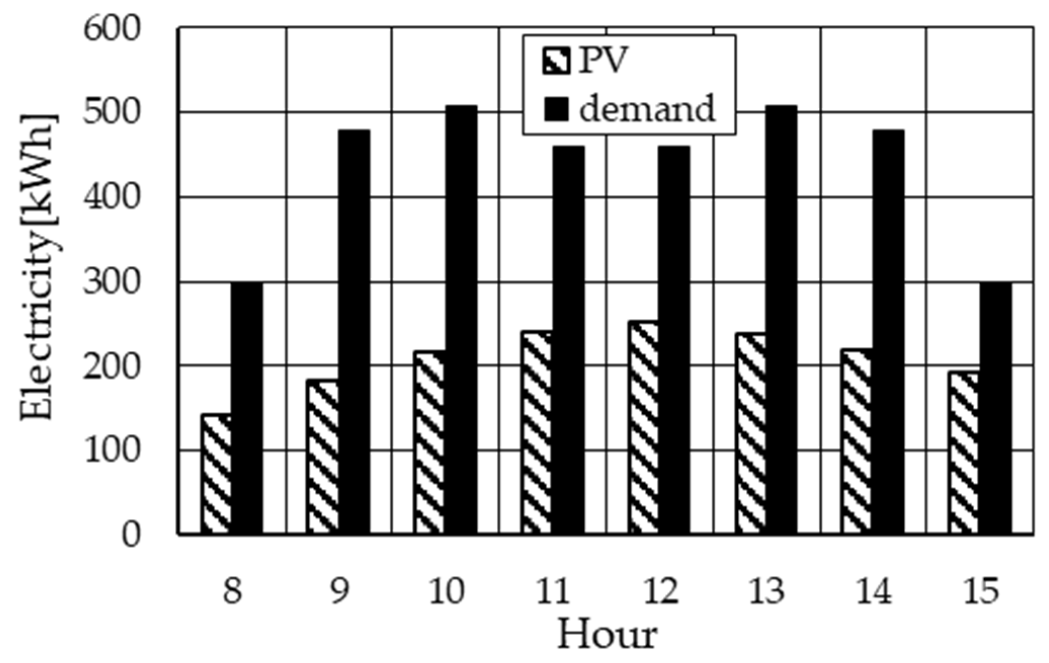
For the analysed model a south-oriented solar installation was adopted, installed on the roof of production halls. The installation capacity was dictated by the average electricity demand during a single shift operation compared to the average energy production from photovoltaic panels. The assumed efficiency of the PV system was 19%.

2.3. Costs of Energy Usage

The costs in individual variants were divided into the cost of gas fuel, electricity, heat and the cost of servicing individual parts of the system.

The cost of electricity was defined as the part depending on the ordered power and energy consumption. According to the adopted assumptions, electricity is purchased only during servicing of cogeneration systems. The cost of consumed electricity was calculated according to the Formula (4) adopted from the supplier in Poland:

$$C_e=N_e·c_{eN}+E_e·\left(c_{eE}+c_{eOZE}+c_{eK}\right)+c_{ae}$$

(4)

where $N_e$ is the power of power grid connection; $c_{eN}$ is the price of power; $E_e$ is the amount of consumed electricity; $c_{eE}$ is the price of electricity (energy and distribution); $c_{eOZE}$ is renewable energy costs; $c_{eK}$ is cogeneration costs and $c_{ae}$ is the fee.

Heat energy was also priced based on the ordered power and the energy consumed. In the adopted model, the cost of heat was determined based on the Formula (5) used by the heat supplier from Poland:

$$C_h=N_h·c_{hN}+Q_h·c_h+c_{ah}$$

(5)

where $N_h$ is the power of heat connection; $c_{hN}$ is the price of heat power (energy and distribution); $Q_h$ is the amount of heat; $c_h$ is the price of heat (energy and distribution) and $c_{ah}$ is the fee.

Costs of natural gas was calculated based on a Formula (6) approved by the gas supplier in Poland:

$$C_g=N_g·c_{gN}+Q_g·c_g+c_{ag}$$

(6)

where $N_g$ is power in fuel, $c_{gN}$ price of power in the fuel; $Q_g$ is the amount of used gas; $c_g$ is the price of fuel (energy and distribution) and $c_{ag}$ is the fee.

To calculate the tax on income for the sale of electricity, the value of taxes was adopted at the level of 19%. This value was adopted based on the average value of taxes in Poland. Energy prices are presented in

Table 2. Costs of energy adopted in model.

Energy	Unit	Price
Electricity	€/kWh	0.13
Heat	€/GJ	10
Natural Gas	€/kWh	0.03
Electricity (sale)	€/kWh	0.057

. The cost of the components was determined based on average market data and is presented in

Table 3. Costs of components of systems adopted in model.

Element	Unit	Cost
CHP	€	730,000
PV	€	550,000
ORC	€	300,000

.

2.4. Profits

Possible income was assumed only in systems type I. It results from the overproduction of electricity and its sale at prices in a competitive market. The adopted nature of the demand for electricity and heat does not allow the achievement of heat utilisation parameters required for high-efficiency cogeneration. Therefore, the benefits of such a solution were not taken into account.

2.5. Financial Efficiency

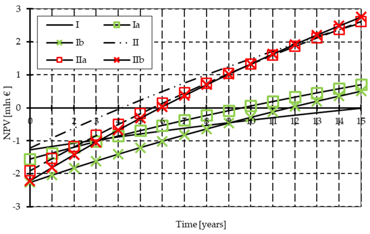
To determine the Dynamic Pay Back Time (DPBT), discounted cash flows (NPV) were used, taking into account investment costs, savings, annual interest and the value of inflation. NPV values were calculated according to the Formula (7):

$$NPV=I+{\displaystyle \sum }_{i=1}^n\frac{S_i}{{\left(1+d\right)}^n}$$

(7)

where $I$ is investment cost; $S$ is savings compared to the standard system; $d$ is the discount rate; $n$ is the year of analysis.

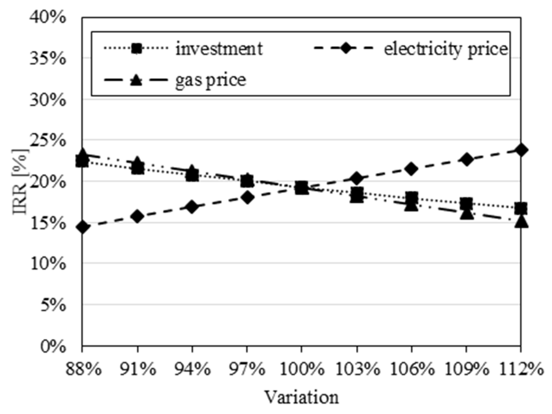
2.6. Sensitivity Analysis

The value of the efficiency indicators is determined for strictly defined investment parameters, such as the size and time distribution of investment expenditures and the assumed economic effects. The result of the analysis, i.e., the values of the indicators, are therefore an assessment of the profitability of the investment for rigidly defined assumptions—valid as at the date of the analysis.

However, the values of individual parameters are subject to a degree of uncertainty, hence the need to perform a sensitivity analysis. It consists in assessing changes in various selected parameters and variables used in the profitability assessment methods, analysing their impact on the profitability of projects and determining the critical values and safety margins determining the profitability level [28,29].

In other words, it consists in calculating the boundary values of selected performance indicators for the assumed confidence levels for determining the main parameters of the investment. Each of the parameters influences the profitability of the investment in a specific way (value of the indicators). The sensitivity analysis determines the impact of the most important investment parameters on its profitability [30,31,32].

The most variable and at the same time, the most influential values determining the profitability of investments are energy prices (both purchase and sale), fuel prices and the benefits of using renewable energy sources.

2.7. The Modelling Procedure

In the scenario method of profitability analysis, several possible cash flows that can be obtained in a given period are determined and assigned a certain probability. Therefore, the predetermined approach to financial forecasting, where the achievement of one value of cash flows is assumed for each period, with the probability of obtaining this result equal to one, is abandoned [33,34].

Before starting the scenario analysis, it was necessary to check the values of the basic statistical meters:

• the Expected Net Present Value—E(NPV),
• standard deviation of the NPV—S(NPV),
• the coefficient of variation—V(NPV).

Values were determined according to the Formulas (8)–(10):

$$E\left(NPV\right)={\displaystyle \sum }_{i=1}^n{p}_i·NP{V}_i$$

(8)

$$S\left(NPV\right)=\sqrt{{\displaystyle \sum }_{i=1}^n{p}_i\ast {(NP{V}_i-E\left(NPV\right))}^2}$$

(9)

$$V\left(NPV\right)=\frac{S\left(NPV\right)}{E\left(NPV\right)}$$

(10)

where $p_i$ is the probability associated with $i$ th possible value; $NP{V}_i$ is $NPV$ value obtained in the case of the $i$-th state of nature; $n$ is the number of possible states of nature (number of obtainable $NPV$ values).

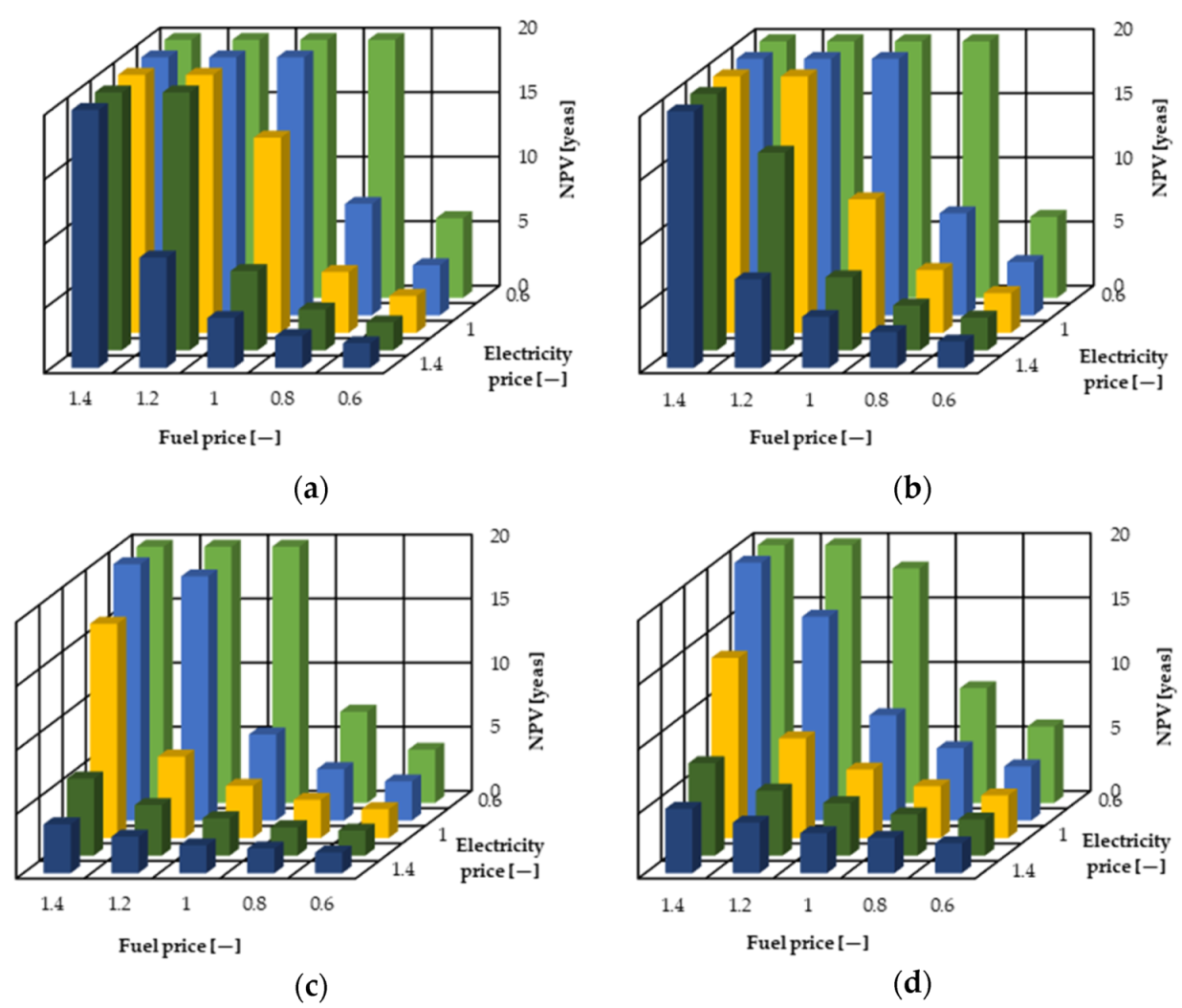
It was decided to adopt three scenarios: optimistic, realistic and pessimistic (

Table 4. Electricity and fuel prices in optimistic, realistic and pessimistic scenarios.

Scenario:	Electricity Price	Fuel Price
optimistic	+10% p.a.	−10% p.a.
realistic	+5% p.a.	−2% p.a.
pessimistic	−10% p.a.	+10% p.a.

). The variables analysed are the price of electricity and the fuel price. These values were selected based on considerations carried out in the first part of this article (introduction). In the first scenario (optimistic) it was assumed that the price of electricity would increase annually by 10%. This assumption is very unlikely, but the scenario analysis is based on adopting extreme solutions. The inverse relationship was adopted for the fuel price—a decrease of 10% annually. In the realistic scenario, market data was used. Based on an analysis of electricity and natural gas suppliers price lists, it was determined that the average annual increase in electricity prices is 3–5%. The scenario assumes a higher value in the range, as prices can be expected to increase along with the increase in the number of distributed electricity producers. Price list analysis also shows that the gas fuel price is decreasing by around 2% per year. In the pessimistic scenario, quite extreme values were again adopted—a decrease in the price of electricity by 10% annually and an increase in fuel prices by 10% a year.

3. Results and Discussion

3.1. PV System during Shift Analysis

The power of the PV system was assumed as 500 kWp. The comparison was made for June when the highest electricity production was achieved with the irradiation database (Figure 5). The average maximum value of energy production was reached at 12 and it was around 250 kWe. Higher nominal power of PV system could not give higher profits. It is caused by two times lower price of electricity at the aftermarket. Analysis of irradiation gives also optimum working hours which was 8–17.

3.2. NPV Analyses

The results of the analysis carried out for the considered variants are shown in Figure 6. There is a significant difference between the time of return on the investment based on one and two gas engines. The solution with the lowest DPBT (equals 4.1 years) was the variant with two gas engines. The longest DPBT (15 years) was achieved for a single-engine variant. This is due to the low selling price of electricity in relation to its purchase. Consequently, an engine operating at nominal power achieves less profit. The confirmation of this explanation can be found in solutions based on photovoltaic systems. In the case of Ia and Ib systems, the energy from PV and ORC is treated as free (recovered) energy, which reduces the payback time to 9.5 and 12.0 years. As a result, the unfavourable energy price ratio is eliminated. For variants IIa and IIb, the payback time is extended to 5.5 and 5.8 years (instead of 4.1 for the basic model), but this variant achieves a higher NPV (after 15 years).

3.3. Sensitivity Results

Sensitivity analysis of the payback period was made (calculated) by the parameter (input) one by one (Figure 7). The payback period are sensitive to the fuel price, electricity prices and investment. The most sensitive parameter is electricity price—the difference between the maximum and minimum payback period is almost 2 years. The highest payback time was achieved with a 12% increase in fuel prices—an increase in almost a year. A 12% change in investment will result in a half-year extension of the payback period.

Sensitivity analysis of the IRR was also made by input one by one (Figure 8). The conventional methodology was applied. In the case of the IRR, it was observed that the price of electricity is the most sensitive parameter. The difference between the highest and lowest values is 9%. A change in the investment value by 12% causes a change in IRR by 2–3%, in the case of the fuel price the difference is 4%.

Figure 9 show the times of return on investment depending on changes in fuel and electricity prices. The values are presented as a value depending on the current price (increased and decreased by 20 and 40%, respectively). The variants based on one gas engine operating at nominal power are most sensitive to changes in these parameters. For variant I, a 20% increase in fuel prices would have to be combined with a 30% increase in electricity prices to maintain the base payback time. In comparison, variant II requires only an 18% increase in electricity prices to maintain a constant DPBT. The implementation of the PV system in Ia reduces the required 28% price decline. No significant changes were noticed in variant IIa.

The change in the prices of certificates for renewable energy sources does not cause significant changes to the DPBT (Figure 10). A 40% decrease in prices caused an increase in DPBT for systems Ia, Ib, IIa and IIb, respectively: 4.3%, 2.0%, 2.4% and 2.0%. These slight differences are a result of the low amount of energy produced from PV in relation to the power of the CHP system.

The analysis was performed for all variants discussed in the paper (I, Ia, Ib, II, IIa, IIb).

Table 5. NPV and probability in optimistic, realistic and pessimistic scenarios for variant II.

Scenario:	NPV						pi
	I	Ia	Ib	II	IIa	IIb
optimistic	156.35	159.97	152.42	172.14	165.58	163.20	25%
realistic	47.94	55.13	46.93	81.51	76.79	76.01	50%
pessimistic	−201.77	−181.81	−192.32	−104.94	−103.13	−98.26	25%

shows the detailed results. A 50% probability of a realistic scenario was assumed, and a 25% probability of an optimistic and pessimistic scenario.

Further analysing the project risk using the scenario method, the expected NPV value, standard deviation NPV and the coefficient of variation for all scenarios were determined. Using the appropriate Formulas and data from Table 4 and Table 5, the calculation results presented in

Table 6. Basic statistical meters for all analysed variants.

Basic Statistical Meters
Variant:	E(NPV)	S(NPV)
I	56.37	114.43
Ia	22.11	108.88
Ib	13.49	109.89
II	57.55	86.98
IIa	54.00	84.15
IIb	54.24	81.70

were obtained.

The maximum standard deviation of NPV was recorded for Variant I (it amounts to over 112 million €) the investment under consideration may therefore bring the NPV by 112 million € lower or higher than the average value estimated at approximately 12.5 million €. This project may therefore turn out to be in fact unprofitable and ineffective. It is characterised by relatively high risk and therefore should not be accepted by investors.

The considerations can be confirmed by the NPV coefficient of variation, which for the example discussed here is over 9. The obtained result suggests that the project has nine times higher risk than any other investment possible for the company, generating relatively more reliable cash flow. It is believed that the NPV coefficient of variation can be compared with the coefficient of variation calculated for another, the so-called average asset that is or maybe at the company’s disposal.

In the case of using two engines (variants II, IIa and IIb), the coefficient of variation is approx. 1.5, which means that the investment risk is acceptable. The lowest standard deviation was calculated for variant IIb. The calculations showed that the investment under consideration may therefore bring the NPV by 82 million € lower or higher than the average value estimated at almost 55 million €.

4. Discussion, Conclusions and Further Research

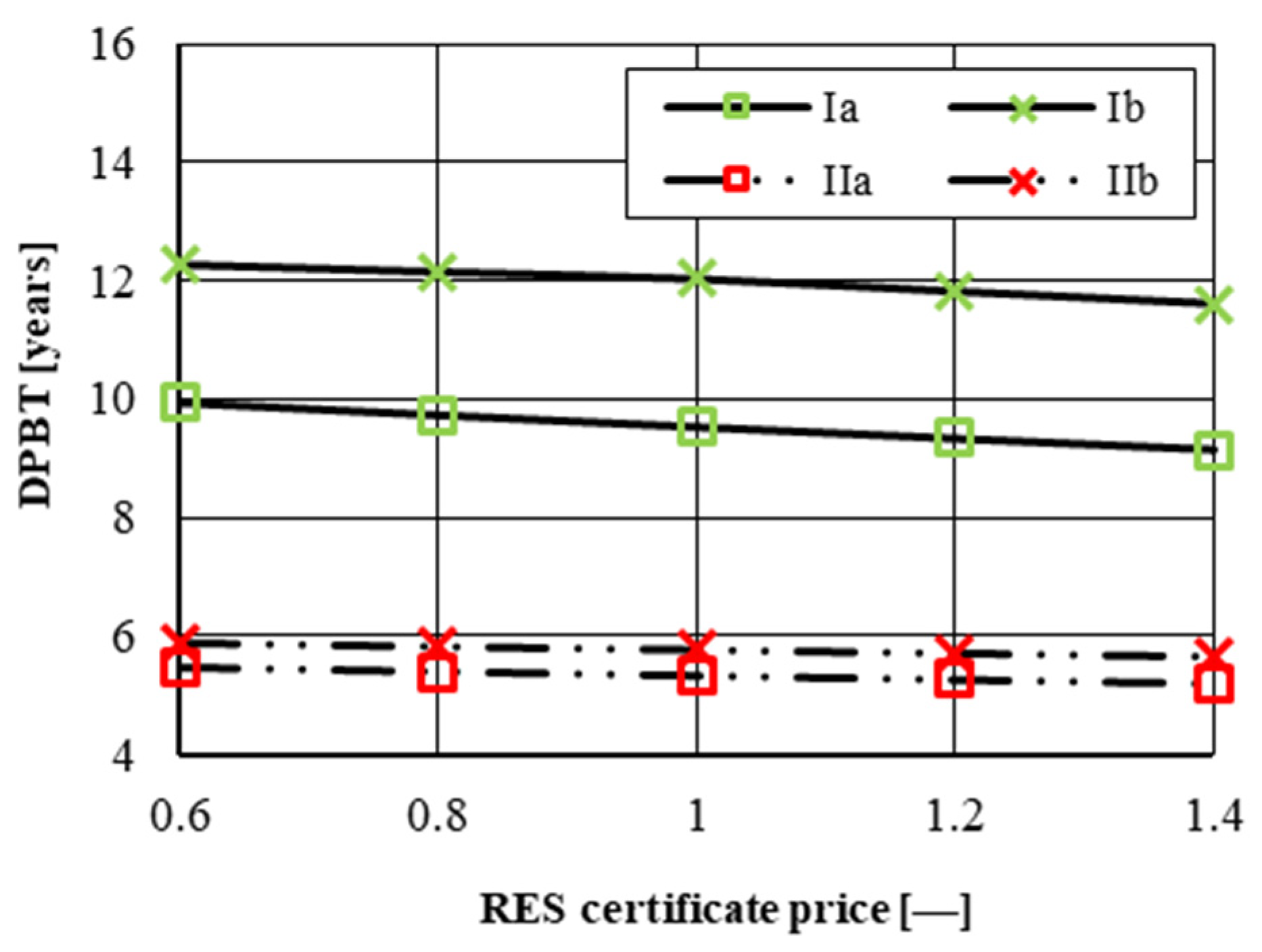
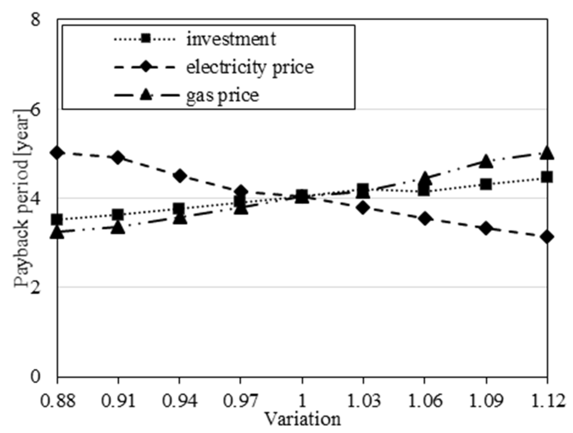
The conducted analysis proved that the use of distributed energy was right in the current situation on the energy price market. The use of small and medium-sized installations for the production of electricity and heat up to 20 MW allows one to avoid ETS fees which increase the costs of energy consumption. In addition, the use of natural gas allows one to reduce CO₂ emissions by half, which is of particular importance for countries whose energy is based on hard coal. The results of the analysis carried out for the model industrial plant showed that with the current energy prices, technology and investment costs, the most profitable system turns out to be a system focused on the current energy demand. The payback time (DPBT) for this solution was calculated at 4.1 years. This is the reason for the unfavourable ratio of fuel prices to electricity purchase prices, which means that its resale brings little profit. The use of photovoltaic systems brings an increase in the NPV value after 15 years, but the payback time is extended due to the significant investment costs. The new plans to purchase energy from PV producers will not give better results. The conducted investment risk analysis also indicated CHP systems focused on the current consumer demand as those with the lowest risk. 10% changes in fuel prices and −10% changes in electricity prices are the least harmful to the II and IIb systems.

Taking into account the results of the work carried out, it is possible to identify further measures to increase the economy and reduce the impact on the environment. First, in the future, it will be required to introduce PV systems with much higher efficiency than 19% today. In addition, it will be necessary to improve the process of their production and at the same time reduce costs. At current prices, the best economical use of PV is to use the generated energy for own needs. Unfortunately, the limited availability of space where their installation is possible limits the power of the installation. Another activity increasing the economics of the modernisation carried out must be to focus on the availability of renewable energy. The nature of the plant’s operation should be as focused as possible while solar energy is available. A complete conversion to solar energy is not possible, but changes in the working hours of the shifts can bring about noticeable changes in the energy cost.

As it was said in the beginning, there are few publications in the scientific literature which discus similar analyses. For example in [17] was shown that using the photovoltaic system is too expensive to get benefits without subsidies. It was proved that the smaller investments are less affected by energy demand uncertainties than the larger ones, which, in turn, provide better performance in terms of expected values [19].

The most important conclusions:

• the most advantageous of the presented solution is the use of a system adjusted to the power of an industrial plant (return on investment in 4th year),
• the least beneficial for the investor are solutions aimed at the use and resale of energy supplemented with photovoltaic panels and an ORC system,
• solutions with variable power are characterised by the lowest investment risk,
• analyses like this are strongly connected with the global market. The developed model will allow for fast and effective NPV analyses in changing conditions on its.

Further research:

• we plan to consider the sensitivity to changing other parameters (such as the interest rate),
• developing a company’s work plan based on the presented model,
• extension of the model to include analysis for enterprises that do not have access to gas networks.