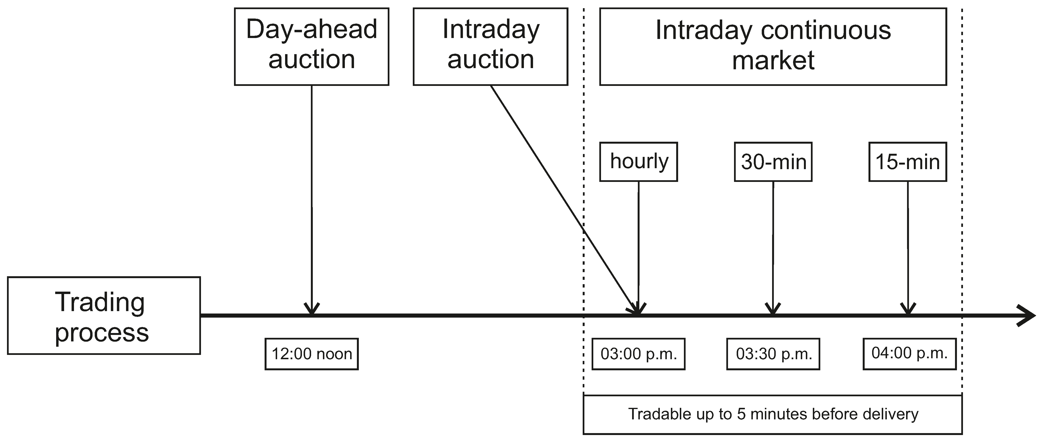
Figure 1.
Typical structure of a trading day on EPEX SPOT. The day-ahead auction is at 12 p.m. (noon). Trading for hourly contracts on the continuous intraday market starts at 3 p.m. and is possible until 5 min before delivery. Until June 2017, trading on the continuous intraday market was possible only up to 30 min before delivery. Afterwards, trading was possible within a control zone until 5 min before delivery.
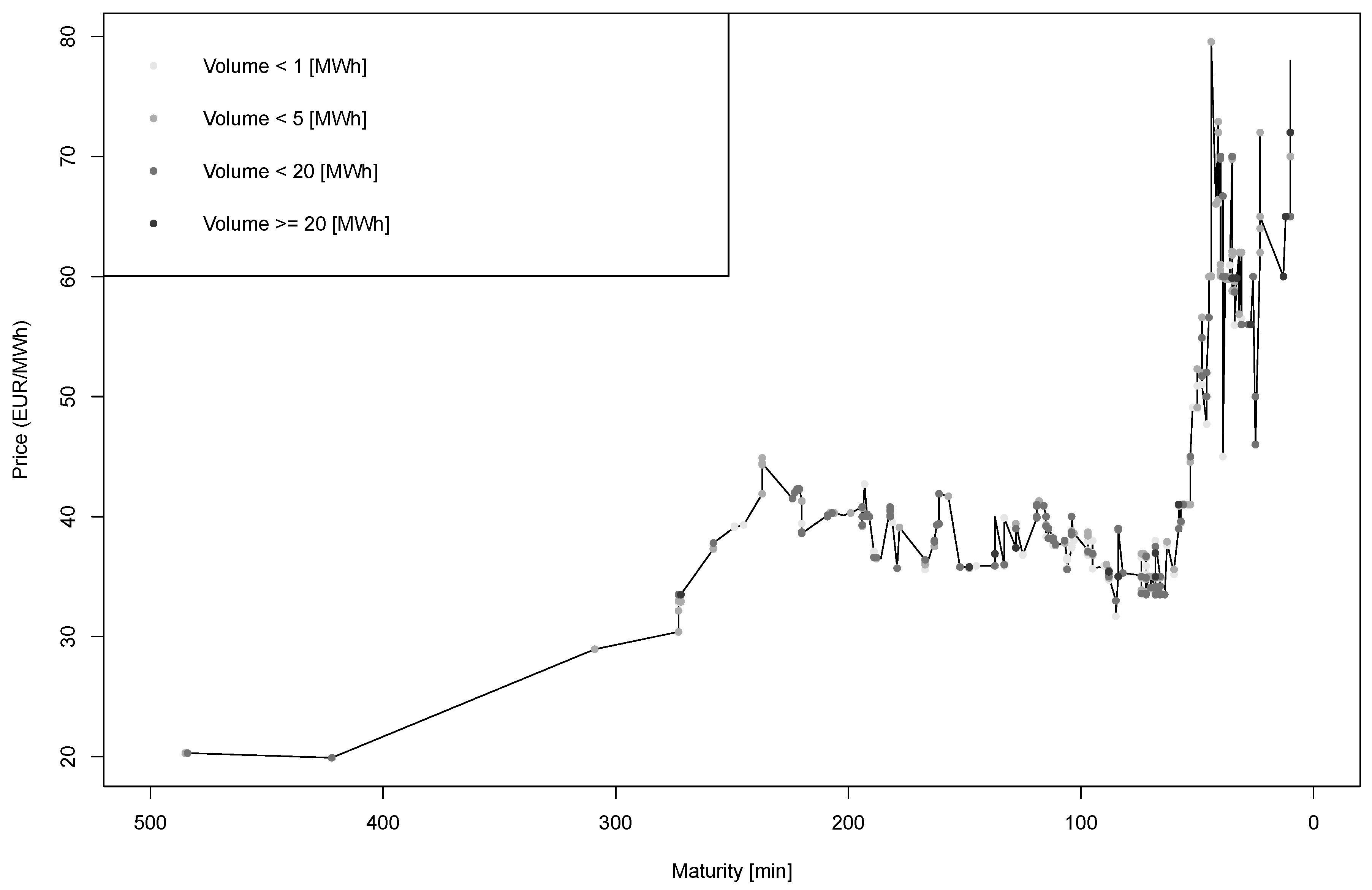
Figure 2.
Selected realized price development of the 00h–01h contract on 23 September 2018 with remaining maturity of the continuous intraday market. The figure illustrates the differences between a classic stock market and the continuous intraday market for electricity. There are large price movements from about EUR 20 to 80 per MWh within the few hours of trading. Furthermore, trades are unevenly distributed and cluster at the end of the period.
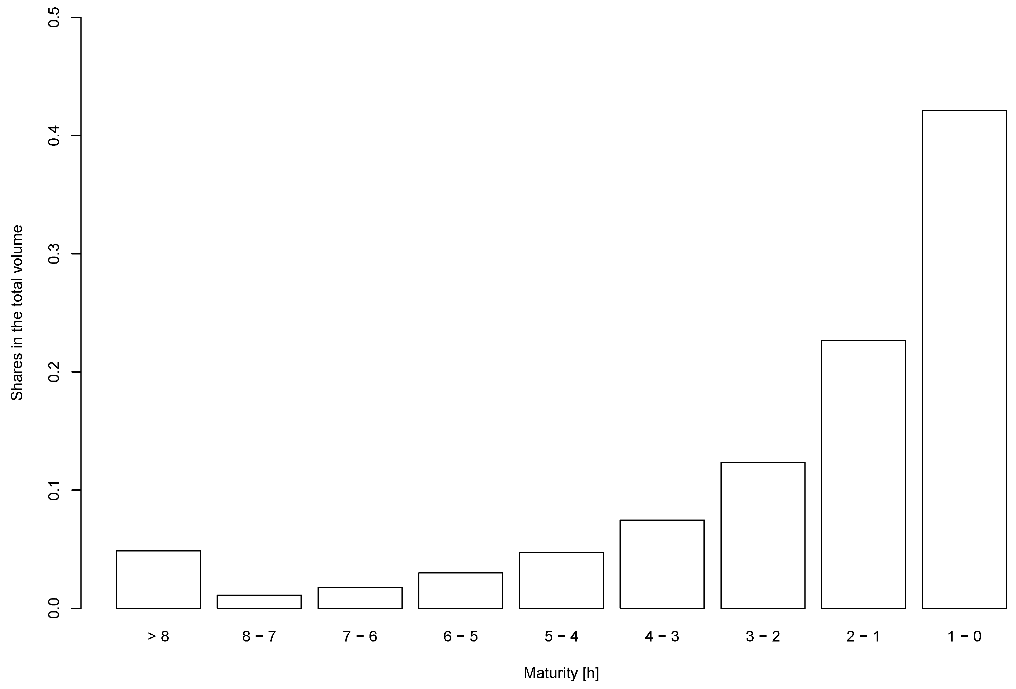
Figure 3.
Relative trading volume of the continuous intraday market per hour before maturity (up to 30 min before delivery). The figure illustrates that trading volume increases sharply with decreasing time to maturity.
Figure 3.
Relative trading volume of the continuous intraday market per hour before maturity (up to 30 min before delivery). The figure illustrates that trading volume increases sharply with decreasing time to maturity.
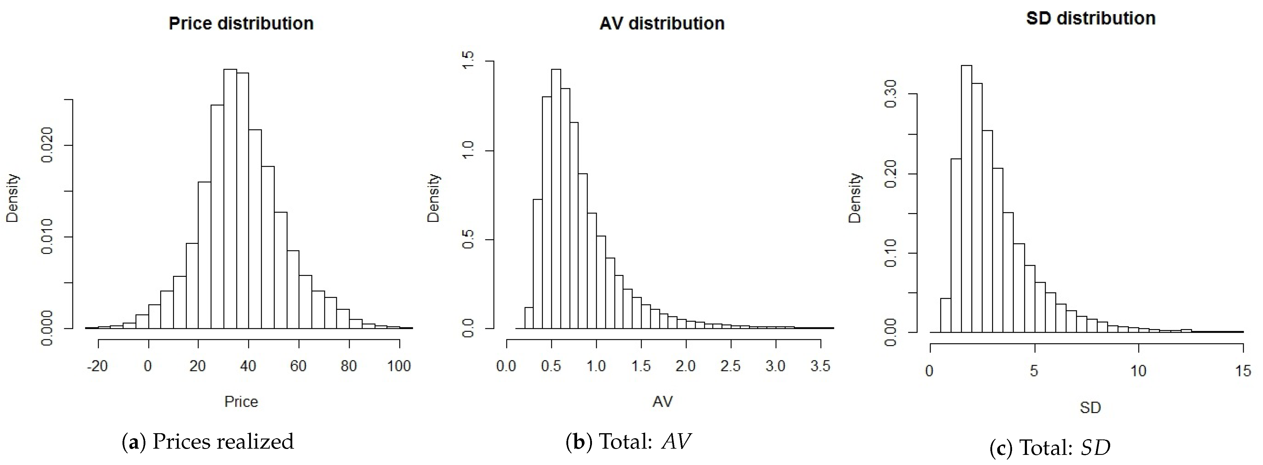
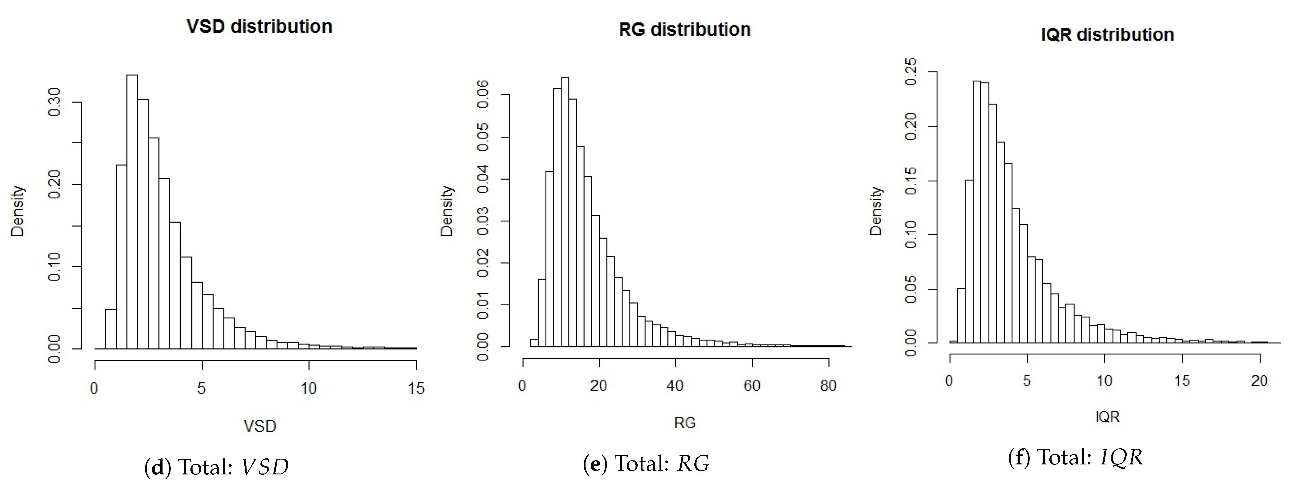
Figure 4.
Histograms of all realized prices (subfigure (a)) and the total five price fluctuation measures (subfigures (b–f)). Extreme values at the tails of the distributions were omitted to provide clarity.
Figure 4.
Histograms of all realized prices (subfigure (a)) and the total five price fluctuation measures (subfigures (b–f)). Extreme values at the tails of the distributions were omitted to provide clarity.
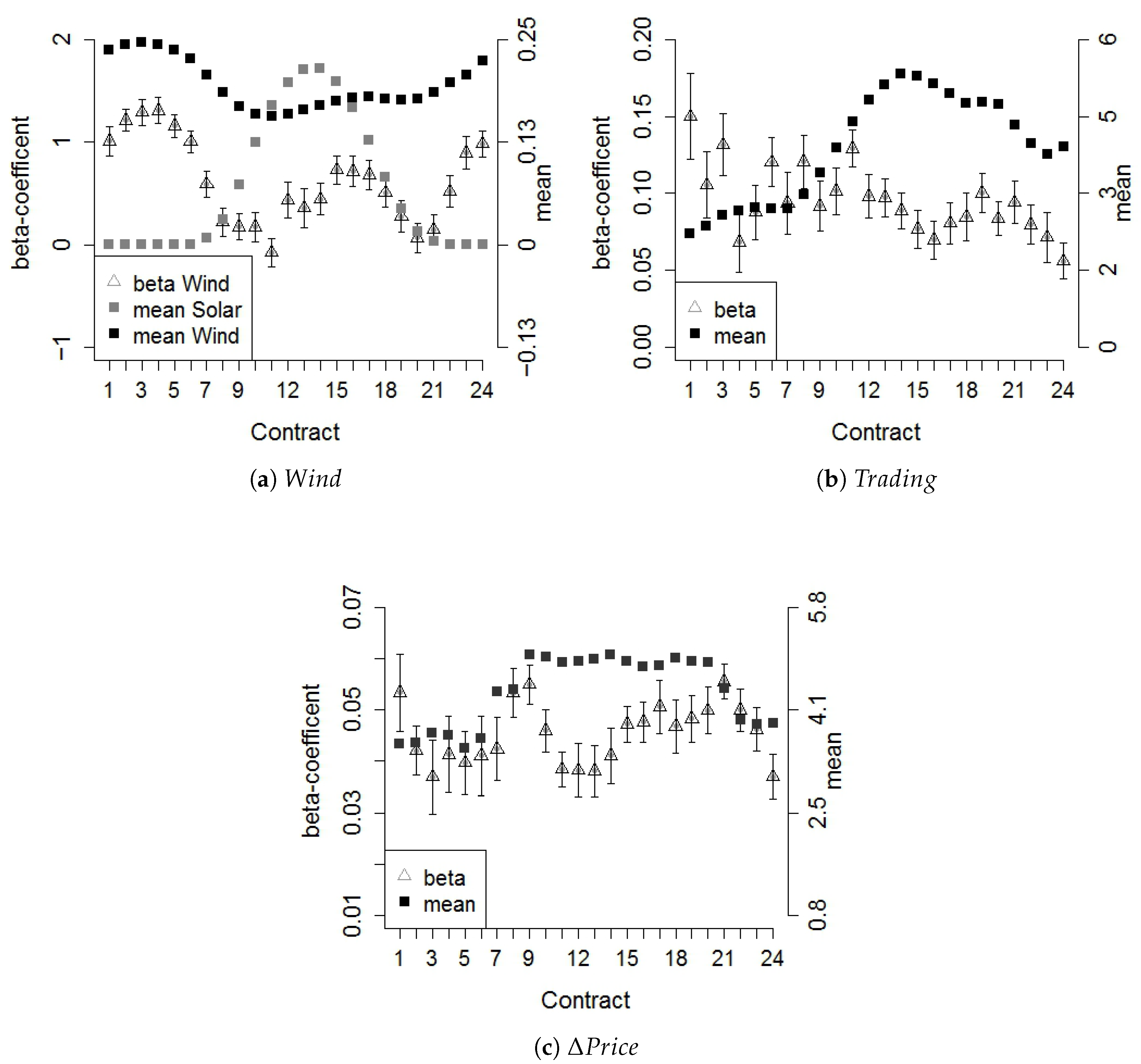
Figure 5.
Regression -coefficients (left axis) for the volume-weighted average standard deviation as the dependent variable, with standard errors, plotted against the corresponding mean (right axis) of the variables separately for the individual hourly contracts. Subfigure (a) shows as the relative wind share of the total consumption (together with the relative solar share of the total consumption ). Subfigure (b) shows as the traded volume of the intraday market in GWh, and Subfigure (c) shows as the absolute price difference of the day-ahead auction price and the volume-weighted average price of the intraday market. Significant influence of coincides with the highest share of wind energy in the overall mix. and were always significant regardless of fluctuating averages.
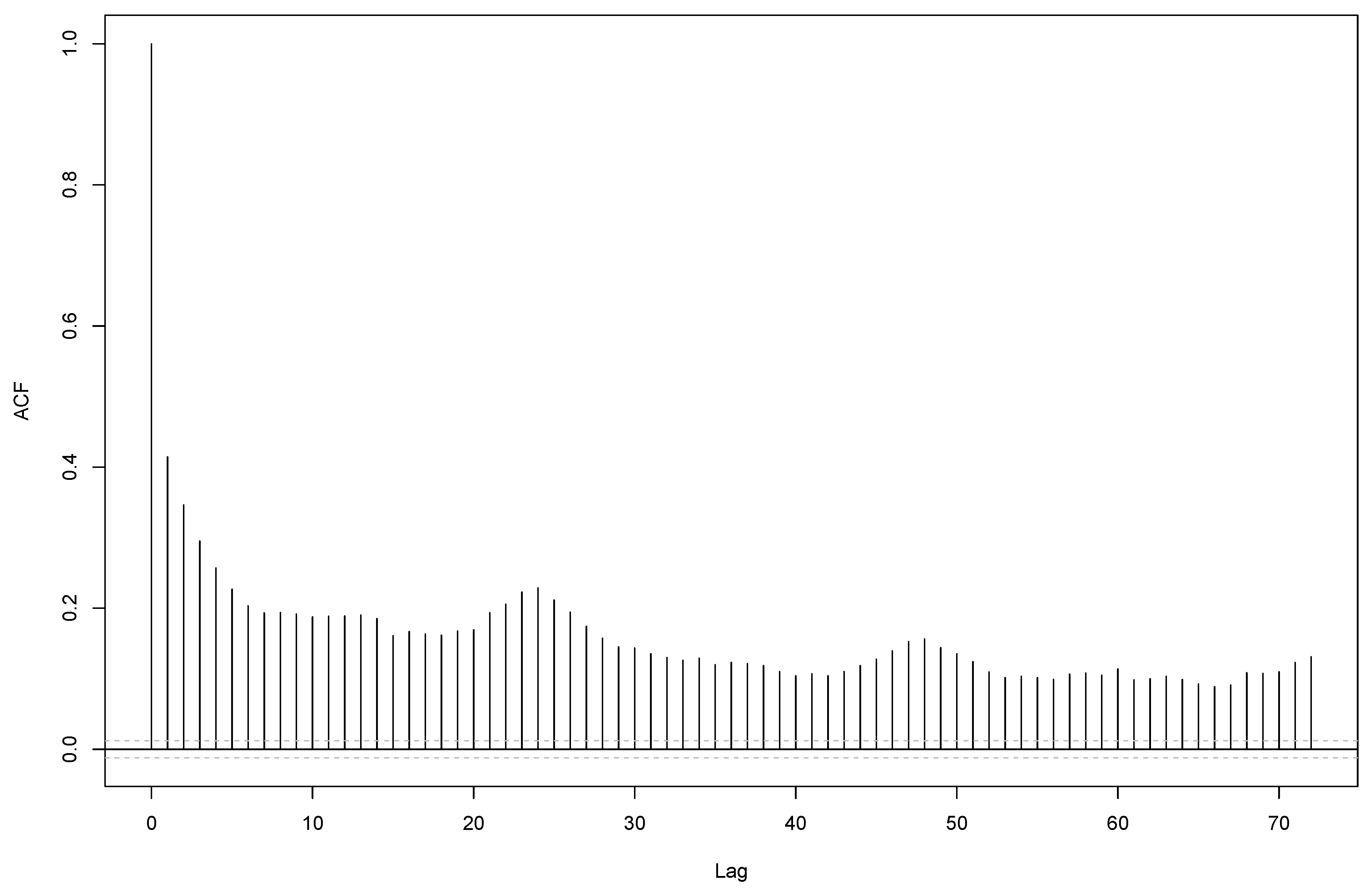
Figure 6.
Autocorrelations of the dispersion measure , the volume-weighted average standard deviation for the final trading hour. Especially for small lags, the correlation is pronounced. A correlation with the price fluctuations of the same hourly contract on the previous day (lag 24) can also be observed.
Table 1.
Descriptive statistics and correlations between the five fluctuation measures. Panel A covers all data and Panel B only the final trading hour of each contract. is the standard deviation of the price differences of consecutive trades. is the standard deviation, the volume-weighted average standard deviation, the range, and the interquartile range of all prices for a single contract. All figures of the descriptive statistics for the measures are given in EUR per MWh.
| | Panel A: Total Price Fluctuations | | Panel B: Last Trading Hour |
|---|
| Transactions | 13.6 millions | | 6.2 millions |
| Volume | 102 TWh | | 44 TWh |
| | | | | | | | | | | | |
| 1% | 0.293 | 0.872 | 0.854 | 4.900 | 0.900 | | 0.245 | 0.606 | 0.594 | 2.800 | 0.600 |
| 25% | 0.527 | 1.862 | 1.854 | 10.25 | 2.200 | | 0.482 | 1.447 | 1.434 | 6.500 | 1.800 |
| Median | 0.706 | 2.682 | 2.681 | 14.40 | 3.300 | | 0.667 | 2.155 | 2.138 | 9.500 | 2.900 |
| Mean | 0.881 | 3.409 | 3.409 | 18.49 | 4.397 | | 0.830 | 2.804 | 2.778 | 12.21 | 3.941 |
| 75% | 0.987 | 3.967 | 3.956 | 21.19 | 5.200 | | 0.943 | 3.304 | 3.278 | 14.00 | 4.800 |
| 99% | 3.393 | 14.88 | 14.84 | 79.58 | 19.80 | | 3.241 | 12.16 | 12.23 | 53.10 | 18.12 |
| SD | 1.310 | 3.215 | 3.682 | 21.88 | 4.367 | | 1.148 | 3.007 | 2.930 | 13.59 | 4.250 |
| Skewness | 38.78 | 9.325 | 28.27 | 21.51 | 7.235 | | 40.19 | 14.15 | 14.10 | 15.25 | 8.857 |
| Kurtosis | 2087 | 193.9 | 1989 | 826.6 | 105.0 | | 2493 | 443.0 | 453.8 | 444.9 | 183.2 |
| 1 | - | - | - | - | | 1 | - | - | - | - |
| 0.542 | 1 | - | - | - | | 0.653 | 1 | - | - | - |
| 0.527 | 0.875 | 1 | - | - | | 0.592 | 0.982 | 1 | - | - |
| 0.872 | 0.810 | 0.754 | 1 | - | | 0.786 | 0.923 | 0.887 | 1 | - |
| 0.256 | 0.843 | 0.739 | 0.516 | 1 | | 0.364 | 0.861 | 0.883 | 0.698 | 1 |
Table 2.
Descriptive statistics of the explanatory variables. is the relative solar share of the total consumption, and is the relative solar forecast error of the total consumption. and are analogously defined as the relative wind share and the relative wind forecast error of the total consumption. is the volume of the total consumption in TWh, is the unsigned relative excess generation over consumption in Germany, is the traded volume of the intraday market in GWh, is the relative share of the volume (buy and sell) traded between Germany and a foreign country and the total traded volume of the intraday market, and is the absolute price difference of the day-ahead auction price and the volume-weighted average intraday price.
| | | | | | | | | | |
|---|
| Min | 0.0000 | 0.00000 | 0.002 | 0.0000 | 0.031 | 0.000 | 0.272 | 0.000 | 0.000 |
| 25% | 0.0000 | 0.00000 | 0.077 | 0.0054 | 0.048 | 0.044 | 2.715 | 0.075 | 1.437 |
| Median | 0.0023 | 0.00030 | 0.154 | 0.0124 | 0.056 | 0.087 | 3.709 | 0.192 | 3.101 |
| Mean | 0.0704 | 0.00525 | 0.191 | 0.0180 | 0.056 | 0.105 | 3.928 | 0.203 | 4.397 |
| 75% | 0.1097 | 0.00639 | 0.270 | 0.0247 | 0.065 | 0.149 | 4.893 | 0.312 | 5.660 |
| Max | 0.5837 | 0.09744 | 0.848 | 0.2829 | 0.079 | 0.536 | 14.31 | 0.718 | 111.3 |
| SD | 0.1090 | 0.00979 | 0.147 | 0.0182 | 0.010 | 0.079 | 1.625 | 0.144 | 5.057 |
Table 3.
Regression results for the five measures for the total price fluctuations. is the standard deviation of the price differences consecutive trades, is the standard deviation, is the volume-weighted average standard deviation, is the range, and is the interquartile range of all observable prices. is the relative solar share of the total consumption, and is the relative solar forecast error of the total consumption. and are analogously defined as the relative wind share and the relative wind forecast error of the total consumption. is the volume of the total consumption in TWh, is the unsigned relative excess generation over consumption in Germany, is the traded volume of the intraday market in GWh, is the relative share of the volume (buy and sell) traded between Germany and a foreign country and the total traded volume of the intraday market, and is the absolute price difference of the day-ahead auction price and the volume-weighted average intraday price. The successive variables represent fixed effects for hour, day, season, year, summer time, and late trading within a control zone. RMSE is the root mean squared error, and MAE is the mean absolute error. The asterisks denote the significance level with *** = 0.1%, ** = 1%, and * = 5%.
| | | | | | |
|---|
| −0.549 *** | 0.494 *** | 0.489 *** | 2.021 *** | 0.737 *** |
| 0.219 * | 0.242 * | 0.321 ** | 0.142 | 0.375 ** |
| −0.170 | −0.560 | −0.555 | −0.175 | −1.293 |
| 0.571 *** | 0.719 *** | 0.767 *** | 0.716 *** | 0.831 *** |
| −1.183 *** | −1.400 *** | −1.596 *** | −1.044 *** | −1.890 *** |
| 1.422 | 0.560 | 0.357 | 3.940 * | −0.226 |
| 0.159 | −0.220 | −0.303 * | −0.023 | −0.333 * |
| −0.012 * | 0.085 *** | 0.088 *** | 0.076 *** | 0.098 *** |
| −0.124 ** | −0.279 *** | −0.349 *** | −0.138 ** | −0.503 *** |
| 0.033 *** | 0.049 *** | 0.047 *** | 0.046 *** | 0.046 *** |
| 0.276 *** | 0.191 *** | 0.203 *** | 0.170 *** | 0.181 *** |
| 0.244 *** | 0.151 *** | 0.172 *** | 0.144 ** | 0.151 ** |
| 0.243 *** | 0.135 ** | 0.146 ** | 0.134 ** | 0.131 * |
| 0.269 *** | 0.158 *** | 0.171 *** | 0.159 *** | 0.145 ** |
| 0.301 *** | 0.158 *** | 0.168 *** | 0.163 *** | 0.128 ** |
| 0.405 *** | 0.237 *** | 0.257 *** | 0.237 *** | 0.241 *** |
| 0.454 *** | 0.334 *** | 0.347 *** | 0.312 *** | 0.332 *** |
| 0.434 *** | 0.357 *** | 0.395 *** | 0.326 *** | 0.379 *** |
| 0.279 *** | 0.271 *** | 0.289 *** | 0.219 *** | 0.313 *** |
| 0.143 *** | 0.147 *** | 0.154 *** | 0.113 *** | 0.160 *** |
| 0.024 * | 0.036 ** | 0.039 ** | 0.012 | 0.030 |
| −0.051 *** | −0.038 ** | −0.041 ** | −0.040 ** | −0.029 |
| −0.066 *** | −0.068 *** | −0.066 *** | −0.071 *** | −0.056 ** |
| −0.029 * | −0.046 ** | −0.044 * | −0.029 | −0.051 * |
| 0.002 | 0.006 | 0.017 | 0.006 | 0.014 |
| 0.024 | 0.016 | 0.029 | 0.022 | 0.020 |
| 0.090 *** | 0.085 *** | 0.094 *** | 0.079 *** | 0.078 ** |
| 0.159 *** | 0.122 *** | 0.140 *** | 0.143 *** | 0.126 *** |
| 0.198 *** | 0.152 *** | 0.175 *** | 0.163 *** | 0.152 *** |
| 0.202 *** | 0.160 *** | 0.181 *** | 0.170 *** | 0.167 *** |
| 0.205 *** | 0.151 *** | 0.168 *** | 0.155 *** | 0.149 *** |
| 0.272 *** | 0.221 *** | 0.243 *** | 0.227 *** | 0.207 *** |
| 0.598 *** | 0.240 *** | 0.376 *** | 0.397 *** | 0.281 *** |
| −0.117 *** | −0.095 *** | −0.094 *** | −0.109 *** | −0.095 ** |
| −0.147 *** | −0.131 *** | −0.128 *** | −0.129 *** | −0.132 *** |
| −0.160 *** | −0.130 *** | −0.131 *** | −0.146 *** | −0.130 *** |
| −0.206 *** | −0.152 *** | −0.149 *** | −0.181 *** | −0.145 *** |
| −0.190 *** | −0.164 *** | −0.162 *** | −0.181 *** | −0.162 *** |
| −0.118 *** | −0.093 *** | −0.095 *** | −0.101 *** | −0.093 *** |
| −0.084 * | −0.070 * | −0.073 * | −0.031 | −0.104 ** |
| −0.104 * | −0.023 | −0.036 | 0.005 | −0.096 * |
| 0.066 | 0.114 *** | 0.118 *** | 0.164 *** | 0.086 ** |
| 2015 | 0.162 ** | −0.035 | −0.023 | −0.168 ** | 0.001 |
| 2016 | −0.008 | −0.151 *** | −0.132 ** | −0.205 *** | −0.097 * |
| 2017 | −0.011 | −0.078** | −0.079 ** | −0.137 *** | −0.045 |
| −0.107 ** | −0.035 | −0.045 | −0.071 * | −0.029 |
| 0.006 | −0.060 | −0.056 | −0.013 | −0.047 |
| adj. | 0.436 | 0.425 | 0.425 | 0.447 | 0.357 |
| 0.364 | 0.430 | 0.434 | 0.412 | 0.523 |
| 0.279 | 0.341 | 0.344 | 0.318 | 0.415 |
| # Observations | 24,893 | 24,906 | 24,913 | 24,904 | 24,926 |
Table 4.
Correlations between the explanatory variables and the volume-weighted average standard deviation . is the relative solar share of the total consumption, and is the relative solar forecast error of the total consumption. and are analogously defined as the relative wind share and the relative wind forecast error of the total consumption. is the volume of the total consumption in TWh, is the unsigned relative excess generation over consumption in Germany, is the traded volume of the intraday market in GWh, is the relative share of the volume (buy and sell) traded between Germany and a foreign country and the total traded volume of the intraday market, and is the absolute price difference of the day-ahead auction price and the volume-weighted average intraday price.
| | | | | | | | | | |
|---|
| 1 | - | - | - | - | - | - | - | - |
| 0.588 | 1 | - | - | - | - | - | - | - |
| −0.229 | −0.128 | 1 | - | - | - | - | - | - |
| −0.100 | −0.055 | 0.367 | 1 | - | - | - | - | - |
| 0.267 | 0.241 | −0.126 | −0.066 | 1 | - | - | - | - |
| 0.029 | −0.026 | 0.441 | 0.157 | −0.486 | 1 | - | - | - |
| 0.343 | 0.386 | 0.033 | 0.160 | 0.494 | −0.287 | 1 | - | - |
| −0.020 | −0.051 | −0.361 | −0.123 | −0.223 | −0.299 | 0.103 | 1 | - |
| 0.007 | 0.089 | 0.286 | 0.217 | 0.084 | 0.114 | 0.273 | −0.134 | 1 |
| −0.062 | 0.021 | 0.364 | 0.182 | 0.107 | 0.093 | 0.269 | −0.193 | 0.550 |
Table 5.
Regression results for the volume-weighted average standard deviation as dependent variable for different models. Panel A contains the coefficients of univariate regressions with additional fixed effects for contracts, day, season, year, daylight saving time, and the possibility of control zone trading later. Panel B contains the coefficients of different multivariate regression designs. is the relative solar share of the total consumption, is the relative wind share of the total consumption, and is the relative solar forecast error of the total consumption. is the unsigned relative excess generation over consumption in Germany, is the traded volume of the intraday market in GWh, is the relative share of the volume (buy and sell) traded between Germany and a foreign country and the total traded volume of the intraday market, and is the absolute price difference of the day-ahead auction price and the volume-weighted average intraday price. FE denotes fixed effects. RMSE is the root mean squared error and MAE is the mean absolute error. The asterisks denote the significance level with *** = 0.1% and ** = 1%.
| | Panel A | Panel B |
|---|
| −0.107 | - | - | - | - | - | - | - | | 0.268 ** | - | - | - |
| (0.148) | | | | | | | | | (0.093) | | | |
| - | 1.361 *** | - | - | - | - | - | 0.908 *** | 0.778 *** | 0.785 *** | 0.833 *** | 0.792 *** | 0.653 *** |
| | (0.086) | | | | | | (0.056) | (0.053) | (0.062) | (0.061) | (0.064) | (0.065) |
| - | - | 4.655 *** | - | - | - | - | - | - | - | −1.486 *** | - | - |
| | | (0.457) | | | | | | | - | (0.323) | | |
| - | - | - | 0.982 *** | - | - | - | - | - | - | - | −0.072 | - |
| | | | (0.193) | | | | | | | | (0.108) | |
| - | - | - | - | 0.155 *** | - | - | 0.049 *** | 0.072 *** | 0.074 *** | 0.076 *** | 0.072 *** | 0.083 *** |
| | | | | (0.006) | | | (0.004) | (0.005) | (0.005) | (0.005) | (0.005) | (0.005) |
| - | - | - | - | - | −0.565 *** | - | - | - | - | - | - | −0.335 *** |
| | | | | | (0.075) | | | | | | | (0.046) |
| - | - | - | - | - | - | 0.059 *** | 0.052 *** | 0.048 *** | 0.047 *** | 0.048 *** | 0.048 *** | 0.047 *** |
| | | | | | | (0.003) | (0.003) | (0.003) | (0.003) | (0.003) | (0.003) | (0.003) |
| FE | yes | yes | yes | yes | yes | yes | yes | no | yes | yes | yes | yes | yes |
| Adj. | 0.125 | 0.224 | 0.145 | 0.136 | 0.220 | 0.139 | 0.363 | 0.367 | 0.418 | 0.419 | 0.420 | 0.418 | 0.422 |
| 0.536 | 0.505 | 0.530 | 0.533 | 0.506 | 0.532 | 0.458 | 0.456 | 0.437 | 0.437 | 0.436 | 0.437 | 0.436 |
| 0.421 | 0.395 | 0.416 | 0.419 | 0.397 | 0.418 | 0.361 | 0.361 | 0.346 | 0.346 | 0.346 | 0.346 | 0.345 |
Table 6.
Results for the volume-weighted average standard deviation as the dependent variable, separated by season and day. Panel A contains the descriptive statistics, and Panel B contains the regression results. is the relative wind share of the total consumption, is the traded volume of the intraday market in GWh, is the relative share of the volume (buy and sell) traded between Germany and a foreign country and the total traded volume of the intraday market, and is the absolute price difference of the day-ahead auction price and the volume-weighted average intraday price. RMSE is the root mean squared error, and MAE is the mean absolute error. The asterisks denote the significance level with *** = 0.1%.
| : | Workday | Sunday/Holiday | Spring | Summer | Autumn | Winter |
|---|
| Panel A: Descriptive Statistics |
| 1% | 0.845 | 0.920 | 0.843 | 0.753 | 0.968 | 0.975 |
| 25% | 1.813 | 2.126 | 1.723 | 1.616 | 2.157 | 2.096 |
| Median | 2.603 | 3.125 | 2.443 | 2.277 | 3.112 | 3.034 |
| Mean | 3.279 | 4.083 | 3.074 | 2.892 | 3.772 | 3.936 |
| 75% | 3.835 | 4.713 | 3.487 | 3.368 | 4.486 | 4.544 |
| 99% | 13.60 | 18.44 | 13.98 | 11.38 | 14.14 | 18.50 |
| SD | 3.059 | 5.894 | 4.687 | 2.877 | 2.902 | 3.837 |
| Skewness | 10.45 | 34.74 | 44.76 | 15.90 | 5.945 | 8.119 |
| Kurtosis | 247.9 | 1762 | 2858 | 527.1 | 79.48 | 136.6 |
| Panel B: Regression Results |
| 0.660 *** | 1.086 *** | 0.788 *** | 0.958 *** | 0.678 *** | 0.611 *** |
| (0.064) | (0.123) | (0.128) | (0.130) | (0.095) | (0.116) |
| 0.083 *** | 0.098 *** | 0.087 *** | 0.093 *** | 0.095 *** | 0.076 *** |
| (0.006) | (0.011) | (0.009) | (0.011) | (0.010) | (0.010) |
| −0.263 *** | −0.464 *** | −0.288 *** | −0.264 *** | −0.138 | −0.464 *** |
| (0.055) | (0.103) | (0.077) | (0.076) | (0.093) | (0.100) |
| 0.054 *** | 0.031 *** | 0.045 *** | 0.061 *** | 0.049 *** | 0.042 *** |
| (0.002) | (0.003) | (0.008) | (0.004) | (0.003) | (0.003) |
| Adj. | 0.418 | 0.454 | 0.386 | 0.398 | 0.401 | 0.424 |
| 0.431 | 0.441 | 0.421 | 0.433 | 0.428 | 0.443 |
| 0.341 | 0.350 | 0.332 | 0.343 | 0.341 | 0.348 |
| # Observations | 21,607 | 4160 | 6529 | 6643 | 6262 | 6331 |
Table 7.
Regression results for the five price fluctuations measures for the last trading hour. is the standard deviation of the price differences consecutive trades, is the standard deviation, is the volume-weighted average standard deviation, is the range, and is the interquartile range of all observable prices. is the relative solar share of the total consumption, and is the relative solar forecast error of the total consumption. and are analogously defined as the relative wind share and the relative wind forecast error of the total consumption. is the volume of the total consumption in TWh, is the unsigned relative excess generation over consumption in Germany, is the traded volume of the intraday market in GWh, is the relative share of the volume (buy and sell) traded between Germany and a foreign country and the total traded volume of the intraday market, and is the absolute price difference of the day-ahead auction price and the volume-weighted average intraday price. RMSE is the root mean squared error, and MAE is the mean absolute error. The asterisks denote the significance level with *** = 0.1%, ** = 1%, and * = 5%.
| | | | | | |
|---|
| −0.246 * | 0.536 *** | 0.523 *** | 2.004 *** | 0.878 *** |
| | (0.106) | (0.122) | (0.119) | (0.120) | (0.134) |
| 0.112 | 0.115 | 0.106 | 0.092 | 0.091 |
| | (0.106) | (0.117) | (0.117) | (0.113) | (0.125) |
| 0.822 | −1.436 | −1.576 * | −0.837 | −2.482 ** |
| | (0.679) | (0.788) | (0.785) | (0.761) | (0.859) |
| 0.475 *** | 0.562 *** | 0.564 *** | 0.602 *** | 0.557 *** |
| | (0.069) | (0.077) | (0.075) | (0.076) | (0.075) |
| −0.733 * | −1.298 *** | −1.342 *** | −1.081 ** | −1.449 *** |
| | (0.312) | (0.367) | (0.363) | (0.350) | (0.397) |
| −5.417 *** | −4.208 * | −3.974 * | −3.837 * | −4.286 * |
| | (0.016) | (0.018) | (0.018) | (0.018) | (0.020) |
| −0.198 | −0.372 ** | −0.374 ** | −0.367 ** | −0.377 ** |
| | (0.132) | (0.141) | (0.139) | (0.138) | (0.143) |
| −0.015 | 0.234 *** | 0.235 *** | 0.240 *** | 0.239 *** |
| | (0.010) | (0.011) | (0.011) | (0.011) | (0.012) |
| 0.040 | −0.192 *** | −0.279 *** | −0.092* | −0.551 *** |
| | (0.041) | (0.049) | (0.050) | (0.046) | (0.059) |
| 0.029 *** | 0.031 *** | 0.031 *** | 0.030 *** | 0.032 *** |
| | (0.002) | (0.002) | (0.002) | (0.002) | (0.002) |
| Fixed Effects | yes | yes | yes | yes | yes |
| Adj. | 0.363 | 0.276 | 0.273 | 0.307 | 0.222 |
| 0.434 | 0.549 | 0.551 | 0.510 | 0.671 |
| 0.338 | 0.438 | 0.440 | 0.402 | 0.539 |
| # Observations | 24,896 | 24,920 | 24,922 | 24,901 | 24,933 |
Table 8.
Results of the forecast regressions for the five measures (the standard deviation of the price differences consecutive trades), (the standard deviation of all trades for a contract), (the volume-weighted standard deviation of all trades for a contract), (the range of all trades for a contract), and (the interquartile range of all trades for a contract). Panel A shows the results of the full regression, and Panel B shows the adjusted of separate regressions, using exclusively the fixed effects, the external variables, and the lagged variables, respectively. , , , , are lagged fluctuations measures for the contracts expired in the previous hours, and is the realized fluctuation measure of the specific contract during the elapsed time of trading. is the traded volume during the elapsed time of trading, is the relative share of the total volume traded between Germany and a foreign country during the elapsed time of trading, is the absolute (unsigned) difference between the last intraday price obtained immediately before the start of the last hour and the day-ahead price, is the absolute (unsigned) difference between the volume-weighted average intraday price obtained during the elapsed time of trading and the day-ahead price, and is the relative forecasted wind energy share of the forecasted total consumption. RMSE is the root mean squared error, and MAE is the mean absolute error. The asterisks denote the significance level with *** = 0.1% and * = 5.0%.
| | | | | | |
|---|
| Panel A: Full Regression Results |
| −0.322 *** | 0.263 *** | 0.271 *** | 0.766 *** | 0.509 *** |
| (0.022) | (0.032) | (0.032) | (0.042) | (0.041) |
| 0.291 *** | 0.192 *** | 0.187 *** | 0.229 *** | 0.132 *** |
| (0.008) | (0.007) | (0.007) | (0.007) | (0.007) |
| 0.119 *** | 0.102 *** | 0.104 *** | 0.117 *** | 0.082 *** |
| (0.007) | (0.007) | (0.007) | (0.007) | (0.007) |
| 0.074 *** | 0.068 *** | 0.068 *** | 0.082 *** | 0.067 *** |
| (0.007) | (0.006) | (0.006) | (0.006) | (0.007) |
| 0.069 *** | 0.060 *** | 0.062 *** | 0.066 *** | 0.050 *** |
| (0.006) | (0.006) | (0.006) | (0.006) | (0.006) |
| 0.038 *** | 0.030 *** | 0.029 *** | 0.035 *** | 0.024 *** |
| (0.006) | (0.006) | (0.006) | (0.006) | (0.006) |
| 0.121 *** | 0.159 *** | 0.142 *** | 0.103 *** | 0.110 *** |
| (0.007) | (0.011) | (0.010) | (0.010) | (0.009) |
| −0.007 * | 0.006 | 0.004 | 0.008 | 0.015** |
| (0.003) | (0.004) | (0.005) | (0.004) | (0.006) |
| 0.064 *** | 0.105 *** | 0.091 *** | 0.096 *** | 0.024 |
| (0.017) | (0.024) | (0.025) | (0.023) | (0.029) |
| 0.008 *** | 0.006 *** | 0.007 *** | 0.010 *** | 0.010 *** |
| (0.001) | (0.001) | (0.001) | (0.001) | (0.002) |
| −0.002 | 0.001 | 0.001 | −0.003 | 0.002 |
| (0.001) | (0.002) | (0.002) | (0.002) | (0.002) |
| 0.121 *** | 0.402 *** | 0.417 *** | 0.399 *** | 0.519 *** |
| (0.024) | (0.035) | (0.035) | (0.033) | (0.047) |
| Adj. | 0.479 | 0.285 | 0.278 | 0.328 | 0.201 |
| 0.365 | 0.516 | 0.521 | 0.475 | 0.654 |
| 0.280 | 0.411 | 0.415 | 0.373 | 0.524 |
| # Observations | 24,496 | 24,609 | 24,642 | 24,524 | 24,675 |
| Panel B: Adjusted of Separate Regressions |
| FE | 0.213 | 0.076 | 0.074 | 0.090 | 0.061 |
| External | 0.183 | 0.155 | 0.154 | 0.175 | 0.122 |
| Lagged | 0.438 | 0.266 | 0.259 | 0.307 | 0.175 |


