Article

Lithium-Ion Battery Parameter Identification via Extremum Seeking Considering Aging and Degradation

by
Iván Sanz-Gorrachategui
*,
Pablo Pastor-Flores
,
Antonio Bono-Nuez
,
Cora Ferrer-Sánchez
,
Alejandro Guillén-Asensio
and
Carlos Bernal-Ruiz
Electric and Communications Department, University of Zaragoza, 50018 Zaragoza, Spain
*
Author to whom correspondence should be addressed.
Energies 2021, 14(22), 7496; https://doi.org/10.3390/en14227496
Submission received: 18 October 2021 / Revised: 3 November 2021 / Accepted: 8 November 2021 / Published: 10 November 2021

Abstract

:
Battery parameters such as State of Charge (SoC) and State of Health (SoH) are key to modern applications; thus, there is interest in developing robust algorithms for estimating them. Most of the techniques explored to this end rely on a battery model. As batteries age, their behavior starts differing from the models, so it is vital to update such models in order to be able to track battery behavior after some time in application. This paper presents a method for performing online battery parameter tracking by using the Extremum Seeking (ES) algorithm. This algorithm fits voltage waveforms by tuning the internal parameters of an estimation model and comparing the voltage output with the real battery. The goal is to estimate the electrical parameters of the battery model and to be able to obtain them even as batteries age, when the model behaves different than the cell. To this end, a simple battery model capable of capturing degradation and different tests have been proposed to replicate real application scenarios, and the performance of the ES algorithm in such scenarios has been measured. The results are positive, obtaining converging estimations both with new and aged batteries, with accurate outputs for the intended purpose.

1. Introduction

Lithium-ion batteries have become the most attractive option for energy storage in recent years, becoming a standard for different applications. Among them, these applications include electric (EV) or hybrid vehicles (HEV), as well as stationary energy storage systems (ESS). This is due to their advantageous qualities such as high voltage, high specific energy, and long cycle life [1,2]. The demand for this battery chemistry has risen up to a 46% of all global production in 2017 [3]. Global lithium production grows on a 2% rate per year since 2000 [4], and it is expected that the total accumulative Second-Life batteries capacity could reach 1000 GWh by the year 2030 [5,6]. Thus, it is necessary to study battery aging in order to estimate the useful life of a battery and to categorize it in the Second-Life market.
A good approach to this problem must study different battery aging mechanisms to understand their features in order to provide reliable estimates for the State of Health (SoH) or the State of Charge (SoC) and to guarantee correct operation of the battery during its life. The diagnosis methods are varied, and there are multiple approaches towards them. According to [7], a subdivision can be made into data-driven, model-based, and hybrid methods [8,9].
Data driven approaches need an substantial amount of data to train statistical or machine learning models. When applying these models, the system is thought of as a black box to which different variables enter as an input, and it is tuned step by step until it outputs the real value.
On the other hand, model-based approaches use a set of differential equations to emulate the dynamic behavior of the system. However, the parameters of the real system may change due to different effects such as temperature or aging, which ultimately depend on the specific usage conditions. Thus, when using model-based approaches to perform SoC or SoH estimation, there is a need for tracking the parameters of the real battery and updating them into the estimation algorithms.
Battery parameter identification and tracking have been extensively studied in the literature. To this end, multiple approaches and models have been considered. Techniques developed and used in these approaches include filters such as Kalman Filters or Particle Filters [10,11]; Least Square methods [12,13]; observers such as Luenberger [14] or H [15]; statistical methods such as Autorregressive models (AR), Hidden Markov Models (HMM) [16], or Gaussian Process Regression (GPR) models [17]; and machine learning techniques such as Support Vector Machine (SVM) or Relevance Vector Machine (RVM) [18,19].
This paper explores the viability of using the Extremum Seeking (ES) algorithm, described initially in [20], as a means to perform Equivalent Circuit Model (ECM) identification in Lithium-ion batteries. In order to perform this, a simple battery model is proposed to serve as the estimation goal. As the main novelty, aging is included; thus, the effectiveness of the ES algorithm can to be tested at different levels, both for new and aged batteries. This will allow determining whether the algorithm is capable of tracking the parameters in the entire lifespan of the cell; thus, the outputs of this algorithm may feed other high-level algorithms such as SoH or SoC estimators.
The paper is organized as follows. Section 2 describes the methodology by explaining battery modelling techniques, the basics of the ES technique, and how to apply it to battery parameter estimation. Section 3 introduces different evaluation metrics and establishes different scenarios in order to test the estimation capabilities of the algorithm by comparing the output of the algorithm with the real values when using both new and aged batteries. Finally, Section 4 discusses the results obtained in the different scenarios, and Section 5 gathers the conclusions of this work.

2. Materials and Methods
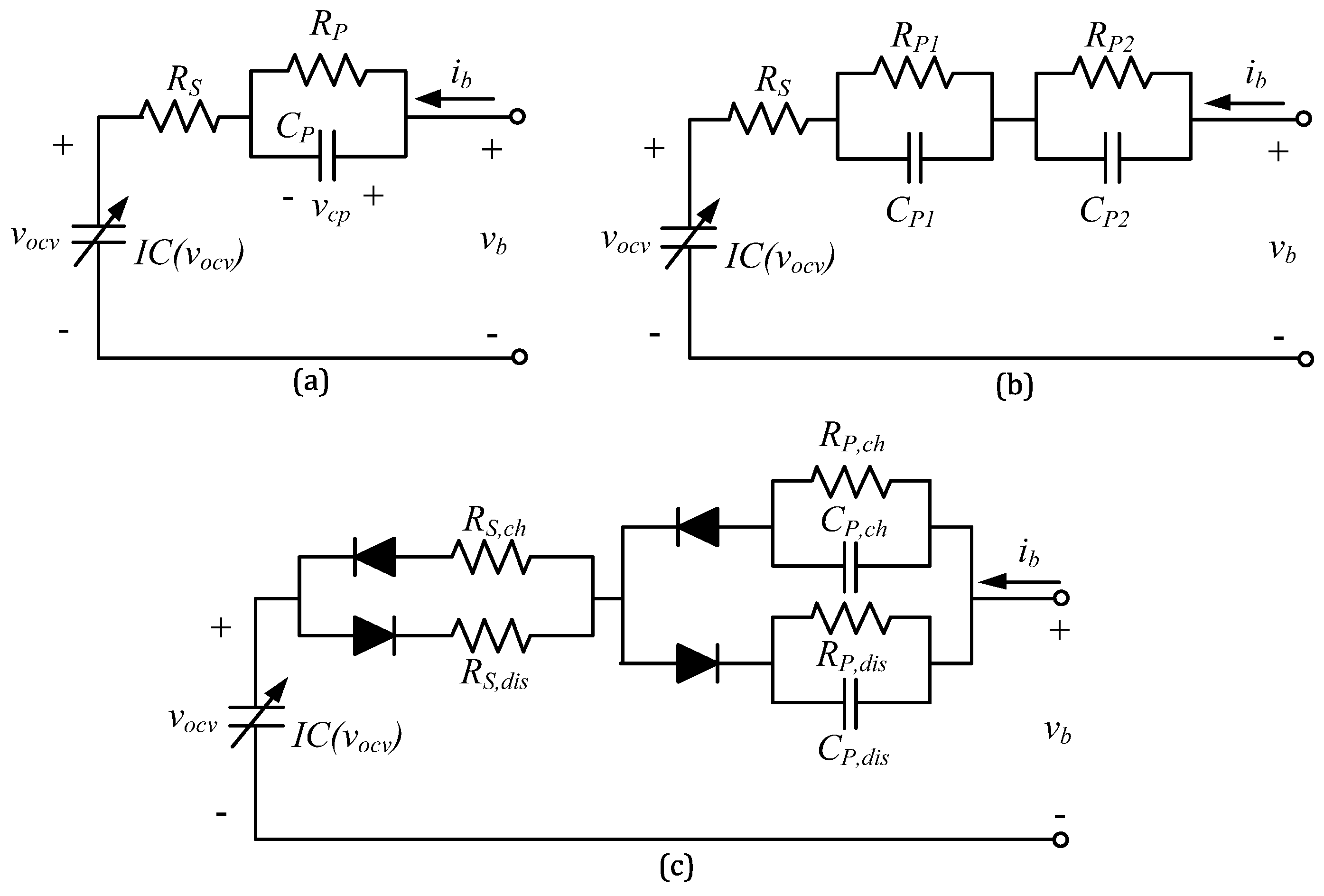
In order to determine whether the Extremum Seeking algorithm is suitable for performing battery model estimation in an embedded application as batteries age, different estimation scenarios are processed, where the algorithm is tested under different conditions. The models and algorithms are described in the following subsections.

2.1. Battery Model

The ES estimation algorithm tries to fit the electrical parameters of the circuital model of a battery cell. Multiple circuital models for batteries have been proposed in the literature. They are commonly divided into two separate parts: the electrical model and the electrochemical model.
The electrical model establishes the output impedance of the battery. Impedance structures are diverse and are selected mainly according to battery chemistry and the prevalent dynamics in application. Sometimes, a simple impedance model with an equivalent series resistance ( R S ) may be enough. However, diffusion effects or different dynamic characteristics are often taken into account. These effects are modeled by RC branches in series with R S . One Time Constant (OTC) or Two Time Constants (TTC) models (Figure 1a,b), including one or two RC branches, respectively, are commonly used for this purpose. Higher complexity impedance models are also proposed in the literature. For example, the authors in [21] used asymmetric impedance structures (Figure 1c) to capture different behaviors when charging ( c h ) and discharging ( d i s ) the batteries. These models are also known as hysteresis models.
For the sake of simplicity, this paper will consider the OTC model. Thus, the output impedance of the battery has been modeled with a series resistance R S and a single parallel R P / / C P branch. The goal of the estimation algorithm will be to obtain an approximation for these electrical parameters.
On the other hand, the electrochemical model of the battery represents the ability of the cell to store energy. An increase in the energy state of the cell is usually related with an increase in the cells’ Open Circuit Voltage ( v o c v ). This is a non-linear relationship and depends on the specific chemistry. This effect is usually modeled with a controlled voltage source for which its voltage depends on the stored charge in the cell. Other elements can be used to model this effect, such as non-linear capacitors [22,23], as is represented in Figure 1. Here, the energy-storage ability of the battery is modeled with the variable capacitor I C ( v o c v ) . This capacitance depends on the open-circuit voltage of the cell and is known as the Incremental Capacity (IC) of the cell.
Incremental Capacity (F) represents the stored charge as a function of voltage (Figure 2). The curves can be obtained from the time-domain charge–discharge waveforms of the cell and is the derivative curve of charge vs. voltage of the cell (Equation (1)) during a single cycle. These curves have been previously described in the literature as a health indicator of the cell [23]. Thus, by using different IC curves as kernels for the electrochemical model, it is possible to imitate cells of the same chemistry at different moments of their life.
IC = δ q ( v ) δ v
This will be useful when designing parameter estimation algorithms in future sections. Initially, an ideal IC curve belonging to a new battery will be used as kernel of the estimation algorithm. It is interesting to observe if the estimation algorithm performs well both for new batteries (with a similar kernel than the estimation algorithm) and for older batteries with an aged kernel.
The complete state-space equations of the OTC battery model are collected in Equation (2) (state equations) and Equation (3) (output equations). This model uses battery current i b as an input and battery voltage v b as an output.
d v c p d t = 1 C P ( i b v c p R P ) d v o c v d t = i b IC ( v o c v )
v b = v o c v + i b R S + v c p
In order to conduct this study, the models are based on the publicly available dataset introduced in [24], which counts with 124 LFP cells. These cells were cycled at 4C as discharge current until their end of life at a controlled ambient temperature of 25 °C. The Incremental Capacity curves used in this study as kernels for the estimation models have been obtained from different cells in said dataset.

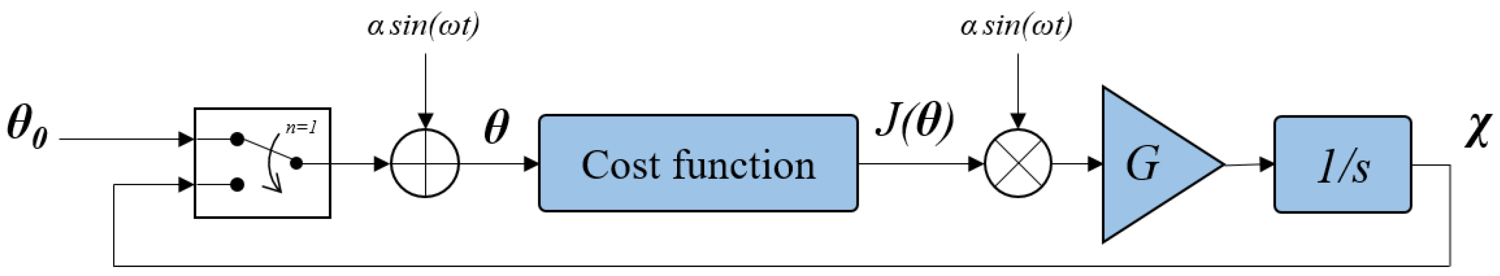
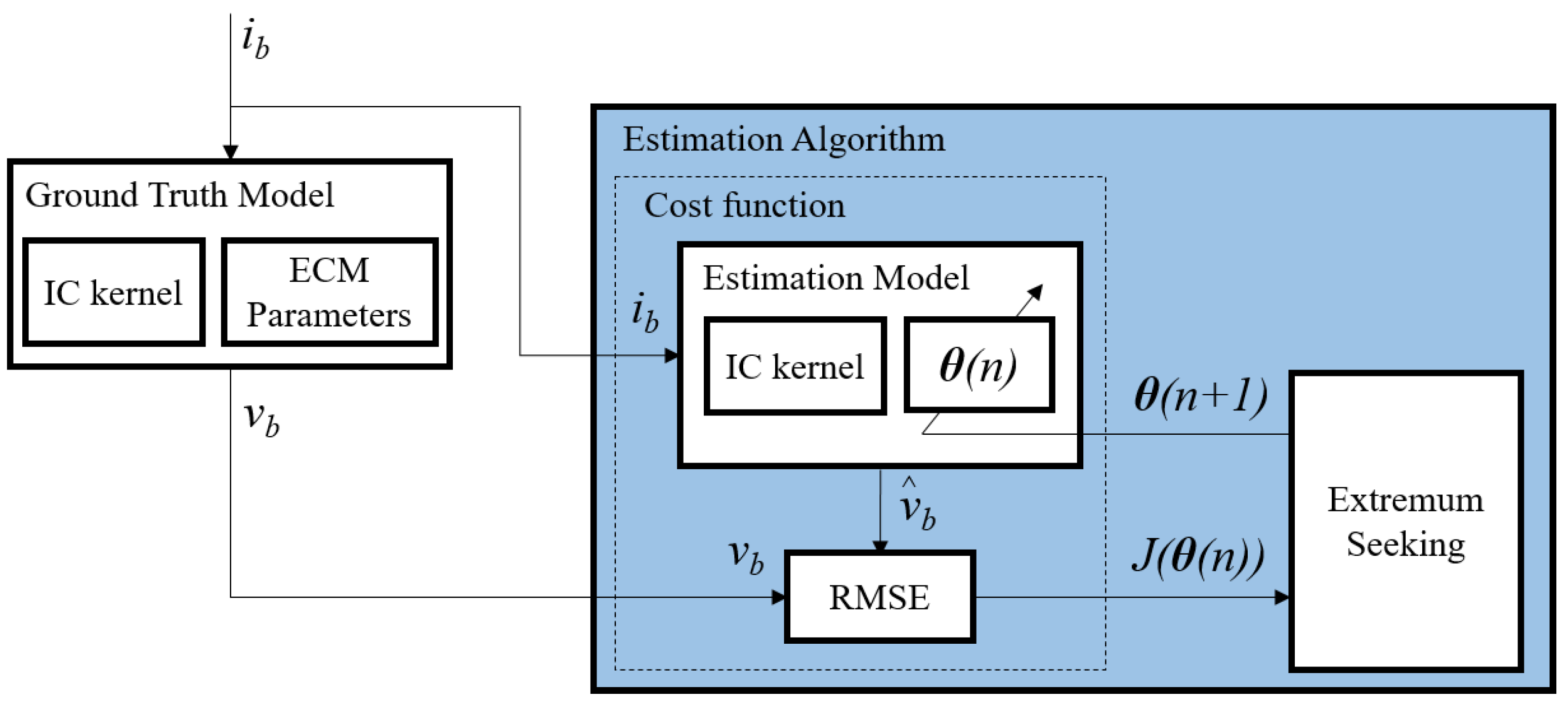
2.2. Extremum Seeking

A basic scheme of the Extremum Seeking algorithm for the estimation of a generic vector parameter θ is shown in Figure 3. This scheme is based in the description in [20,25,26]. A summarized explanation is developed below.
The goal of the algorithm is to converge to a minimum of the cost function J ( θ ) , thus obtaining the best values for the elements in θ that accomplishes that goal. The algorithm starts with an initial set of parameters θ 0 and injects a sinusoidal perturbation ( α s i n ω t ) to them. Afterwards, the cost function J ( θ ) is applied. The resulting cost is then multiplied by another sinusoidal signal and a gain factor G. This results in an estimate of the gradient of the cost function with respect to the parameter vector θ . This estimate is then integrated and added to the original perturbation signal.
The basic equations that describe the behavior of this algorithm for the i-th parameter are described below:
χ i = α i G s i n ( ω i t + π 2 ) J ( θ )
θ i = χ i + α i s i n ( ω i t π 2 )
where the angular frequencies ω i for each of the i parameters must be large enough to ensure convergence (compared to the dynamics of the system). Additionally, they must be different and must not be multiples. The cost function J ( θ ) will converge to a neighborhood of its minimum provided that the hyperparameters G, α i , and ω i are selected adequately [26].
These equations may be discretized to be implemented in a real-time processing scheme (see Equations (6) and (7)), where n is the iteration index, and Δ T is the sampling period.
χ i [ n + 1 ] = χ i [ n ] + α i G Δ T s i n ( ω i n + π 2 ) J ( θ [ n ] )
θ i [ n + 1 ] = χ i [ n + 1 ] + α i s i n ( ω i n π 2 )
This ES algorithm can be applied to battery parameter estimation by following the scheme in Figure 4. Here, the goal is to estimate the parameters of the ECM model of the battery; thus, θ = [ R S ; R P ; C P ] .
In the figure, a battery model (ground truth model) imitates a real battery. This model counts with a fixed set of ECM parameters ( R S , R P , and C P ), which are the estimation targets, and an IC kernel. A current waveform ( i b ) is applied to it, and the output voltage waveform is obtained ( v b ). The estimation algorithm receives the signals i b and v b and uses them in the cost function to obtain J ( θ ) .
Inside this function, there is another battery model named the estimation model, which uses the vector θ as circuital parameters. On each iteration n, the estimation algorithm uses i b as the input of the estimation model with parameters θ [ n ] and then compares its output voltage waveform, v ^ b ( θ [ n ] ) , with the voltage output of the ground truth model, v b . The RMS error between these voltage waveforms is then computed as the resulting cost J ( θ [ n ] ) in Equation (8):
J ( θ [ n ] ) = 1 K k = 1 K ( v b ( k ) v ^ b ( k , θ [ n ] ) ) 2
where k is the time-domain variable related to the waveforms, and K is the number of samples of the voltage waveforms.
The electrical parameters of the estimation model, θ = [ R S ; R P ; C P ] , are then adjusted for the following iteration n + 1 to fit those in the ground truth model so that the error can be minimized by following the Extremum Seeking algorithm described in Equations (6) and (7). When the cost function converges, the parameters in that iteration are considered as output parameters.
It is important to note that the estimation algorithm only varies the electrical parameters and not the IC kernel. Thus, it seems evident that the closer the kernels are between both models, the more accurate the parameter estimation. In the following section, different test scenarios have been evaluated to determine whether this is a very critical effect or if it can be neglected.

3. Results

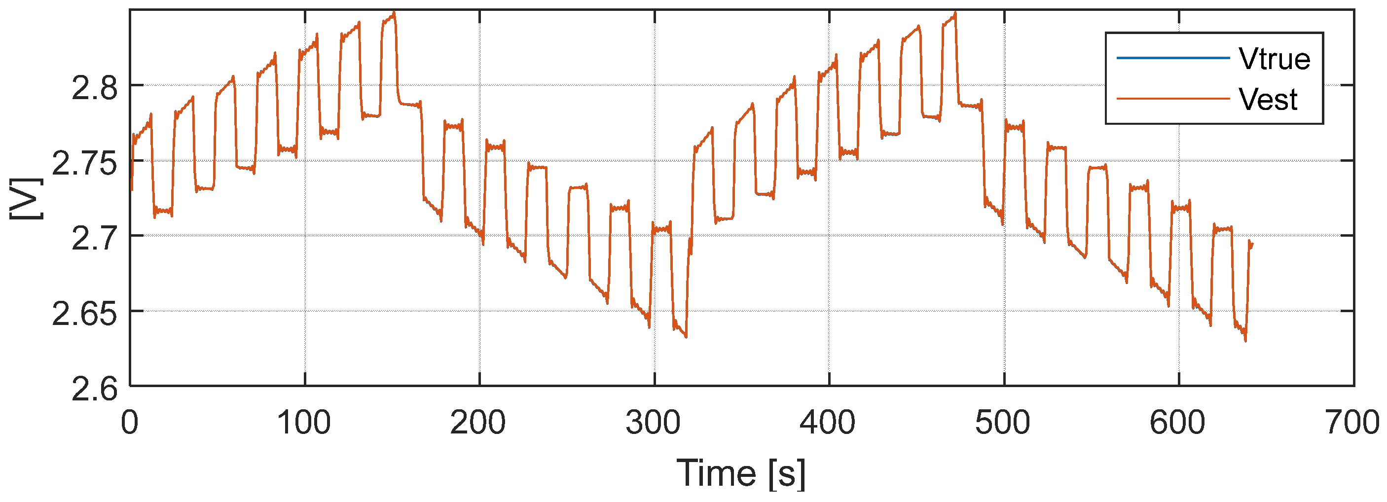
3.1. Evaluation Metrics
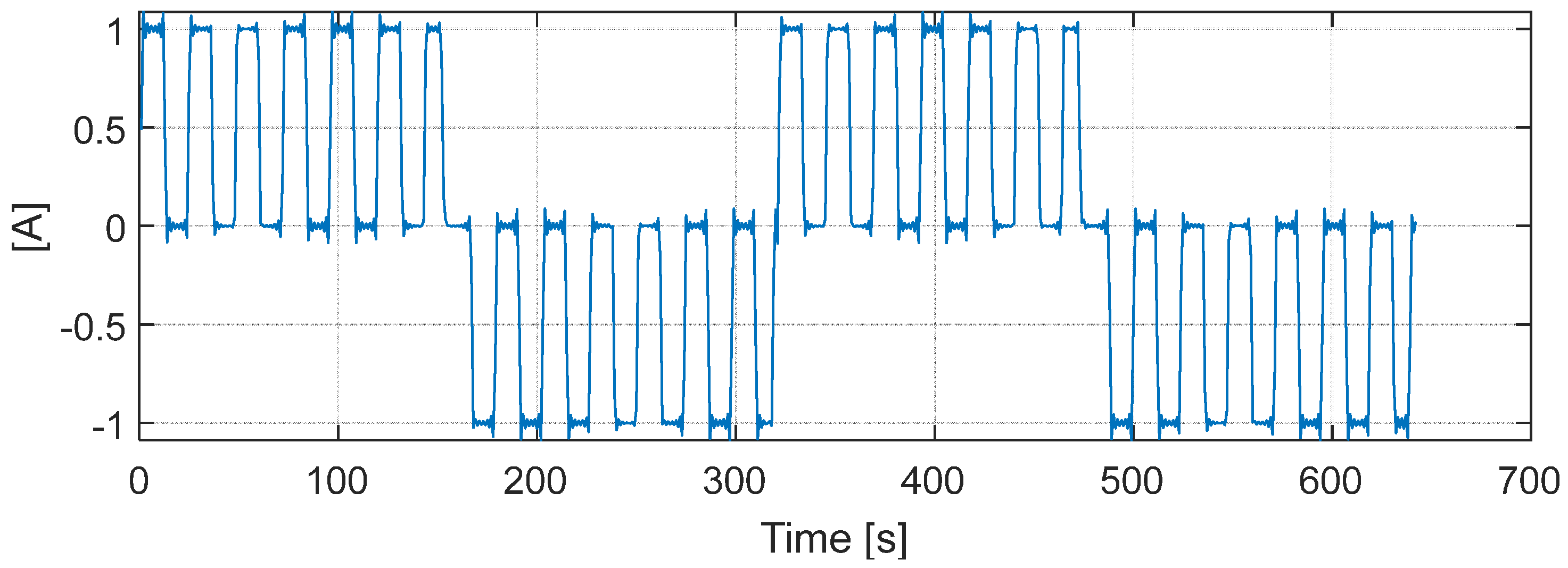
In order to evaluate the performance of the algorithm, the output parameters are compared to the real parameters. These parameters are of different natures ( R S , R P , and C P ); thus, the Mean Relative Error (MRE) has been considered (Equation (9)). Here, x represents the electrical parameters, and x ^ represents its estimation. The real values of the parameters to be estimated in the following subsections are contained in Table 1.
MRE ( % ) = x x ^ x · 100
However, this metric is only obtainable in a design stage when the true battery parameters are known. In real applications, only the error in the voltage waveform can be obtained. Thus, the Root Mean Square Error (RMSE) of the voltage waveform is also provided (see Equation (10)). Here, v b represents the voltage samples measured between time k = 1 and k = K . The variable v ^ b represents the voltage output of the algorithm with the final estimated electrical parameters.
RMSE = 1 K k = 1 K ( v b ( k ) v ^ b ( k ) ) 2

3.2. Test Scenarios

How the ES algorithm estimates the parameters of the circuital model ( R S , R P , and C P ) has already been introduced, but it does not modify the IC kernel. In order to validate the estimation approach, different scenarios with the same current input are considered. The input current waveform is shown in Figure 5.
In each scenario, the kernel of the estimation model inside the ES algorithm remains the same, but the kernel of the ground truth model changes, emulating different cells and aging. The first cycle of cell #43 in the dataset introduced in Section 2.1 has been used as the ground truth model across all the simulations in this work. The different scenarios are introduced below.
  • The ground truth model and the estimation model have the same kernel, which belongs to the first cycle of the same cell (same cell and same aging).
  • The ground truth kernel and the estimation kernel belong to the same cell but at different moments of its life (same cell and different aging).
  • The ground truth kernel and the estimation kernel belong to different cells at different moments of their life (different cell and different aging).

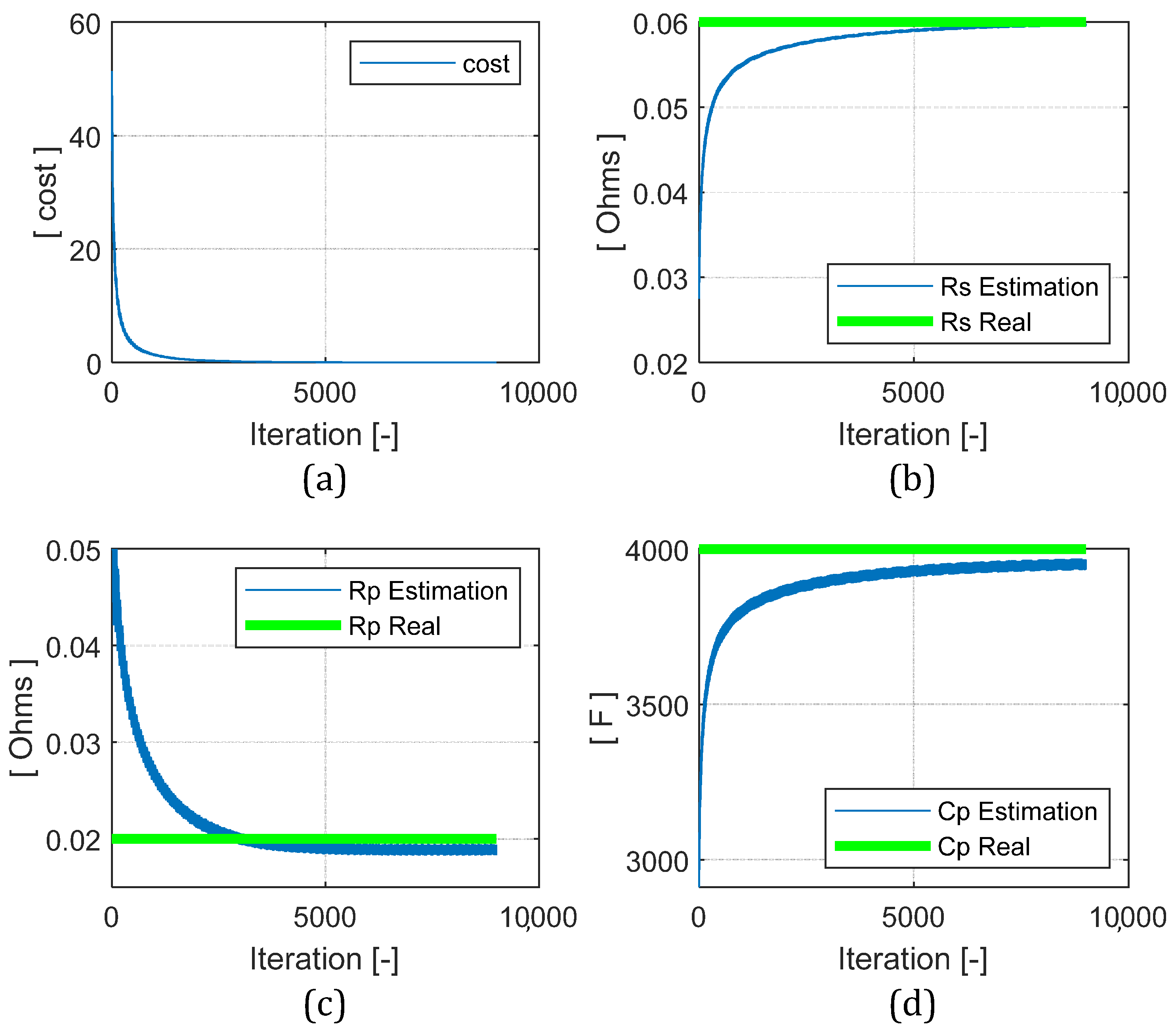
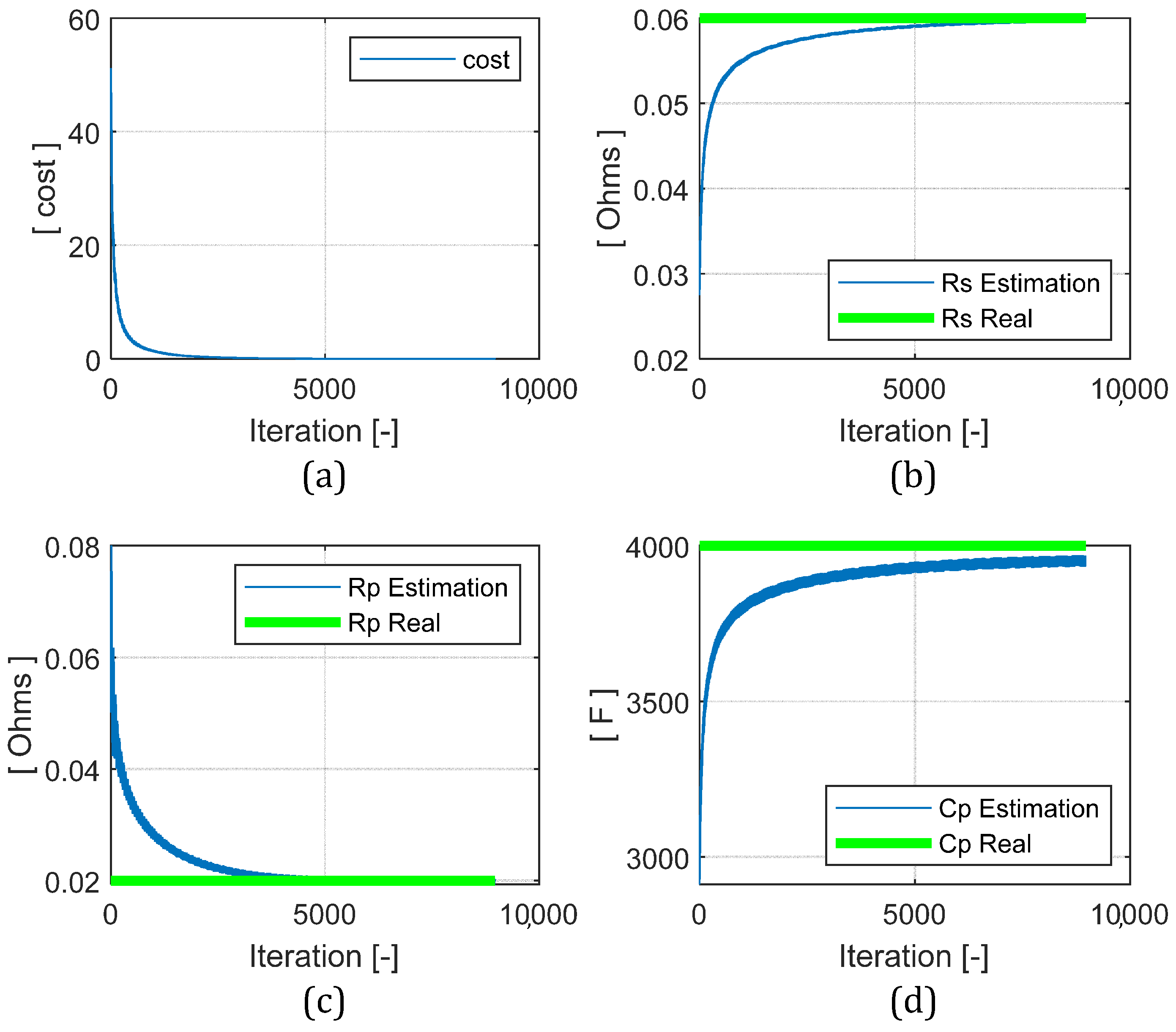
3.3. Same Cell and Same Aging

In this case, the exact same IC kernel is used in both the ground truth model and the estimation model. The goal of this first test is to adjust the hyperparameters of the ES algorithm and to determine if it converges properly, as the final output of both models should be the same since they share the same kernel.
The evolution of the cost function and of each of the electrical parameters along the iterations of the ES algorithm is shown in Figure 6. We can appreciate how each parameter converges appropriately to their real values, although the estimate for C P seems to be biased, as it stabilizes at a value different than the real value. Regardless of this effect, the estimates are accurate and achieves errors below 1% for all the parameters, as it may be appreciated in Table 2.
Additionally, this table contains the RMSE metric for the voltage estimation, which is also very accurate. The voltage waveform obtained with the obtained ECM model ( V e s t ) is compared to the actual voltage waveform ( V t r u e ) in Figure 7.

3.4. Same Cell; Different Aging

In this case, the IC kernels originate from the same cell in the dataset but at different moments of its life. The kernel in the estimation model still belongs to a new battery, whereas the kernel in the ground truth model belongs to the aged cell. The goal here is to determine whether the algorithm is still capable of estimating electrical parameters even when the voltage-capacity curve changes due to aging or, on the contrary, if it will adjust the parameters to better fit the voltage waveform even if that means failing at estimating their actual value.
The evolution of the cost and the electrical parameters is shown in Figure 8. We can appreciate the fact that the convergence is similar to the previous scenario. A small bias in the convergence of the parameter R P can be observed here as well. In this case, however, the estimate for the parameter R P overshoots the actual value of the parameter, and this results in a worst final estimate.
The results obtained in this scenario are collected in Table 3. We can appreciate how the error metrics are still good but are worse than those obtained in the previous scenario in a minor percentage. The relative error for the R P parameter is substantially worse due to the overshoot introduced earlier, but it is still accurate. The final absolute value for this parameter is 19.37 m Ω , compared to the actual 20 m Ω .
The voltage output with the final electrical parameters is very similar to the previous scenario (Figure 7), since this small variation in the parameters does not seem to have a big impact in the final voltage error.

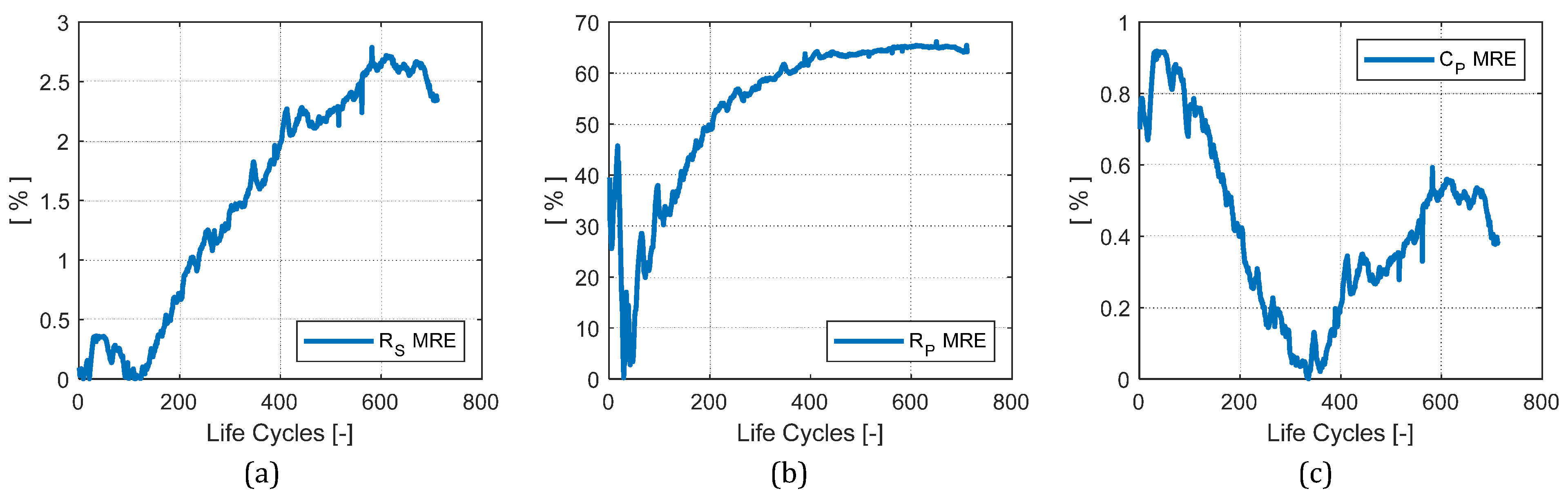
3.5. Different Cell and Different Aging

In order to obtain the error metrics of the algorithm in a wider and more realistic case of application, multiple virtual batteries with many different kernels, both aged and new, have been used as ground truth models in this scenario. The average error metrics for each of the parameters and for the voltage waveforms across the entire set of batteries have been obtained to this end. The final results are collected in the Table 4.
As it may be appreciated, the error metrics are, in general, worse than those obtained in the previous scenarios. This makes sense, since here the parameters are being estimated for multiple cells across the dataset and at different moments of their lives. The estimation of the parameters R S and C P is still accurate, with averaged errors below 2%. On the other hand, MRE has increased quite substantially in the case of the R P parameter, up to a 79.5%. In order to better analyze these results, the evolution of the error is studied. Specifically, the MRE evolution for one of the cells in the dataset (cell #110) is depicted in Figure 9.
As it may be appreciated, at the beginning of battery life, the errors for the R S and the R P parameters are low. This is reasonable, since the IC kernel has not aged that much at this point of the life of the cell and is very similar to the IC kernel of the estimation model. As the cell ages, the IC kernel of the ground truth model evolves and becomes different compared to the kernel of the estimation model; thus, the error for the parameters increases. The error for the C P parameter follows a different trend, but it is low in the entire life-span (always below 1%).

4. Discussion

The error metrics obtained in the first and the second scenarios are below 1% for series resistance ( R S ) and parallel capacitance ( C P ) and around 3% in the worst case for the parallel resistance ( R P ). Furthermore, the error in the voltage waveform is extremely low in both cases, below 1 m V . These results show that the proposed algorithm is capable of estimating accurately the electrical parameters of the cells when the kernels are similar and indicate that the ES method is valid for such purposes. The second scenario also shows that the proposed algorithm is capable of tracking battery parameters even when the kernel of the battery has degraded (varying slightly from its initial form); thus, it is a valid option when dealing with old cells.
When analyzing the performance of the algorithm across the entire dataset, with both new and aged cells (third scenario), the results for R S and C P are still good. Even though the error metrics for these parameters evolve and change as the batteries age, the error always remains below 3% in the case of R S and 1% in the case of C P . As a comparison, the results in [13] show a relative error of up to a 3.5% when estimating R S ; thus, the results obtained here are reasonable in comparison. In the case of R P , the relative error increases substantially as batteries age. The error in this parameter varies dramatically along the lifespan (Figure 9b) and averages at 79.5% across the entire dataset. On the contrary, the estimation of the voltage waveform is still very accurate (5.2 mV). Thus, it can be concluded that the exact value of R P does not have a representative impact in the voltage waveform estimation. In order to increase its impact, different current patterns including pulses with other shapes may be used as inputs for capturing different dynamics in the current–voltage response of the cell.

5. Conclusions

This paper has described an Extremum-Seeking based parameter estimation algorithm aimed at electrical parameter estimation in lithium-ion batteries. The algorithm fits voltage waveforms between a real battery and a tunable model and adjusts the internal parameters of said model to minimize the error in the waveforms.
The proposed model includes a kernel that captures battery aging; thus, the performance of the algorithm has been studied in different scenarios across the lifespan of different cells to validate the approach.
In general, it has been observed that the algorithm performs accurate estimations for all the parameters when the batteries are new, and the internal model of the estimation algorithm is closer to the real battery. This trend has also been observed when estimating the parameters of that same cell but with an aged kernel.
However, the error for some specific parameter increases when estimating multiple different cells across their entire lifespan. This suggests the possibility for improvements by considering other input current waveforms. Thus, as a future line of work, other current patterns ( i b ) may be selected as inputs in order to better capture the relevance of R P in the waveforms. The inclusion of different current-shaped pulses with other dynamics should increase the relevance of dynamical parameters in the model ( R P and C P ); thus, better estimation errors should be expected.

Author Contributions

Conceptualization, I.S.-G. and P.P.-F.; software, C.F.-S. and P.P.-F.; validation, I.S.-G. and A.B.-N.; investigation, C.F.-S.; data curation, P.P.-F.; writing—original draft preparation, I.S.-G. and A.G.-A.; writing—review and editing, A.G.-A.; supervision, A.B.-N. and C.B.-R.; funding acquisition, C.B.-R. All authors have read and agreed to the published version of the manuscript.

Funding

This research was funded by Diputación General de Aragón under the RIS3 Aragón research line, co-founded by the program FEDER Aragón 2014–2020 with grant number LMP16_18 “Desarrollo de Sistemas de Almacenamiento Híbridos e Inteligentes (SAHI)”.

Conflicts of Interest

The authors declare no conflict of interest.

References

  1. Han, X.; Lu, L.; Zheng, Y.; Feng, X.; Li, Z.; Li, J.; Ouyang, M. A review on the key issues of the lithium ion battery degradation among the whole life cycle. eTransportation 2019, 1, 100005. [Google Scholar] [CrossRef]
  2. Xiong, R.; Pan, Y.; Shen, W.; Li, H.; Sun, F. Lithium-ion battery aging mechanisms and diagnosis method for automotive applications: Recent advances and perspectives. Renew. Sustain. Energy Rev. 2020, 131, 110048. [Google Scholar] [CrossRef]
  3. Ambrose, H.; Kendall, A. Understanding the future of lithium: Part 1, resource model. J. Ind. Ecol. 2020, 24, 80–89. [Google Scholar] [CrossRef]
  4. Martin, G.; Rentsch, L.; Höck, M.; Bertau, M. Lithium market research—Global supply, future demand and price development. Energy Storage Mater. 2017, 6, 171–179. [Google Scholar] [CrossRef]
  5. Stringer, D.; Ma, J. Where 3 Million Electric Vehicle Batteries Will Go When They Retire. Bloom. Businessweek 2018, 27. Available online: https://www.bloomberg.com/news/features/2018-06-27/where-3-million-electric-vehicle-batteries-will-go-when-they-retire (accessed on 7 November 2021).
  6. Haram, M.H.S.M.; Lee, J.W.; Ramasamy, G.; Ngu, E.E.; Thiagarajah, S.P.; Lee, Y.H. Feasibility of utilising second life EV batteries: Applications, lifespan, economics, environmental impact, assessment, and challenges. Alex. Eng. J. 2021, 60, 4517–4536. [Google Scholar] [CrossRef]
  7. Hu, X.; Xu, L.; Lin, X.; Pecht, M. Battery Lifetime Prognostics. Joule 2020, 4, 310–346. [Google Scholar] [CrossRef]
  8. Li, K.; Zhou, P.; Lu, Y.; Han, X.; Li, X.; Zheng, Y. Battery life estimation based on cloud data for electric vehicles. J. Power Sources 2020, 468, 228192. [Google Scholar] [CrossRef]
  9. Li, S.; He, H.; Su, C.; Zhao, P. Data driven battery modeling and management method with aging phenomenon considered. Appl. Energy 2020, 275, 115340. [Google Scholar] [CrossRef]
  10. Plett, G.L. Extended Kalman filtering for battery management systems of LiPB-based HEV battery packs: Part 3. State and parameter estimation. J. Power Sources 2004, 134, 277–292. [Google Scholar] [CrossRef]
  11. Plett, G.L. Sigma-point Kalman filtering for battery management systems of LiPB-based HEV battery packs: Part 2: Simultaneous state and parameter estimation. J. Power Sources 2006, 161, 1369–1384. [Google Scholar] [CrossRef]
  12. Xia, B.; Lao, Z.; Zhang, R.; Tian, Y.; Chen, G.; Sun, Z.; Wang, W.; Sun, W.; Lai, Y.; Wang, M.; et al. Online Parameter Identification and State of Charge Estimation of Lithium-Ion Batteries Based on Forgetting Factor Recursive Least Squares and Nonlinear Kalman Filter. Energies 2018, 11, 3. [Google Scholar] [CrossRef] [Green Version]
  13. Giordano, G.; Klass, V.; Behm, M.; Lindbergh, G.; Sjöberg, J. Model-based lithium-ion battery resistance estimation from electric vehicle operating data. IEEE Trans. Veh. Technol. 2018, 67, 3720–3728. [Google Scholar] [CrossRef]
  14. Tang, X.; Liu, K.; Lu, J.; Liu, B.; Wang, X.; Gao, F. Battery incremental capacity curve extraction by a two-dimensional Luenberger–Gaussian-moving-average filter. Appl. Energy 2020, 280, 115895. [Google Scholar] [CrossRef]
  15. Yu, Q.; Xiong, R.; Lin, C.; Shen, W.; Deng, J. Lithium-Ion Battery Parameters and State-of-Charge Joint Estimation Based on H-Infinity and Unscented Kalman Filters. IEEE Trans. Veh. Technol. 2017, 66, 8693–8701. [Google Scholar] [CrossRef]
  16. Piao, C.; Li, Z.; Lu, S.; Jin, Z.; Cho, C. Analysis of real-time estimation method based on hidden markov models for battery system states of health. J. Power Electron. 2016, 16, 217–226. [Google Scholar] [CrossRef] [Green Version]
  17. Sahinoglu, G.O.; Pajovic, M.; Sahinoglu, Z.; Wang, Y.; Orlik, P.V.; Wada, T. Battery state-of-charge estimation based on regular/recurrent Gaussian process regression. IEEE Trans. Ind. Electron. 2017, 65, 4311–4321. [Google Scholar] [CrossRef]
  18. Yu, Z.; Xiao, L.; Li, H.; Zhu, X.; Huai, R. Model Parameter Identification for Lithium Batteries Using the Coevolutionary Particle Swarm Optimization Method. IEEE Trans. Ind. Electron. 2017, 64, 5690–5700. [Google Scholar] [CrossRef]
  19. Xiong, R.; Tian, J.; Shen, W.; Sun, F. A Novel Fractional Order Model for State of Charge Estimation in Lithium Ion Batteries. IEEE Trans. Veh. Technol. 2019, 68, 4130–4139. [Google Scholar] [CrossRef]
  20. Wei, C.; Benosman, M. Extremum seeking-based parameter identification for state-of-power prediction of lithium-ion batteries. In Proceedings of the 2016 IEEE International Conference on Renewable Energy Research and Applications (ICRERA), Birmingham, UK, 20–23 November 2016; pp. 67–72. [Google Scholar] [CrossRef]
  21. Coleman, M.; Lee, C.K.; Zhu, C.; Hurley, W.G. State-of-Charge Determination From EMF Voltage Estimation: Using Impedance, Terminal Voltage, and Current for Lead-Acid and Lithium-Ion Batteries. IEEE Trans. Ind. Electron. 2007, 54, 2550–2557. [Google Scholar] [CrossRef]
  22. Muthuswamy, B.; Banerjee, S. Introduction to Nonlinear Circuits and Networks; Springer: Berkeley, CA, USA, 2018. [Google Scholar]
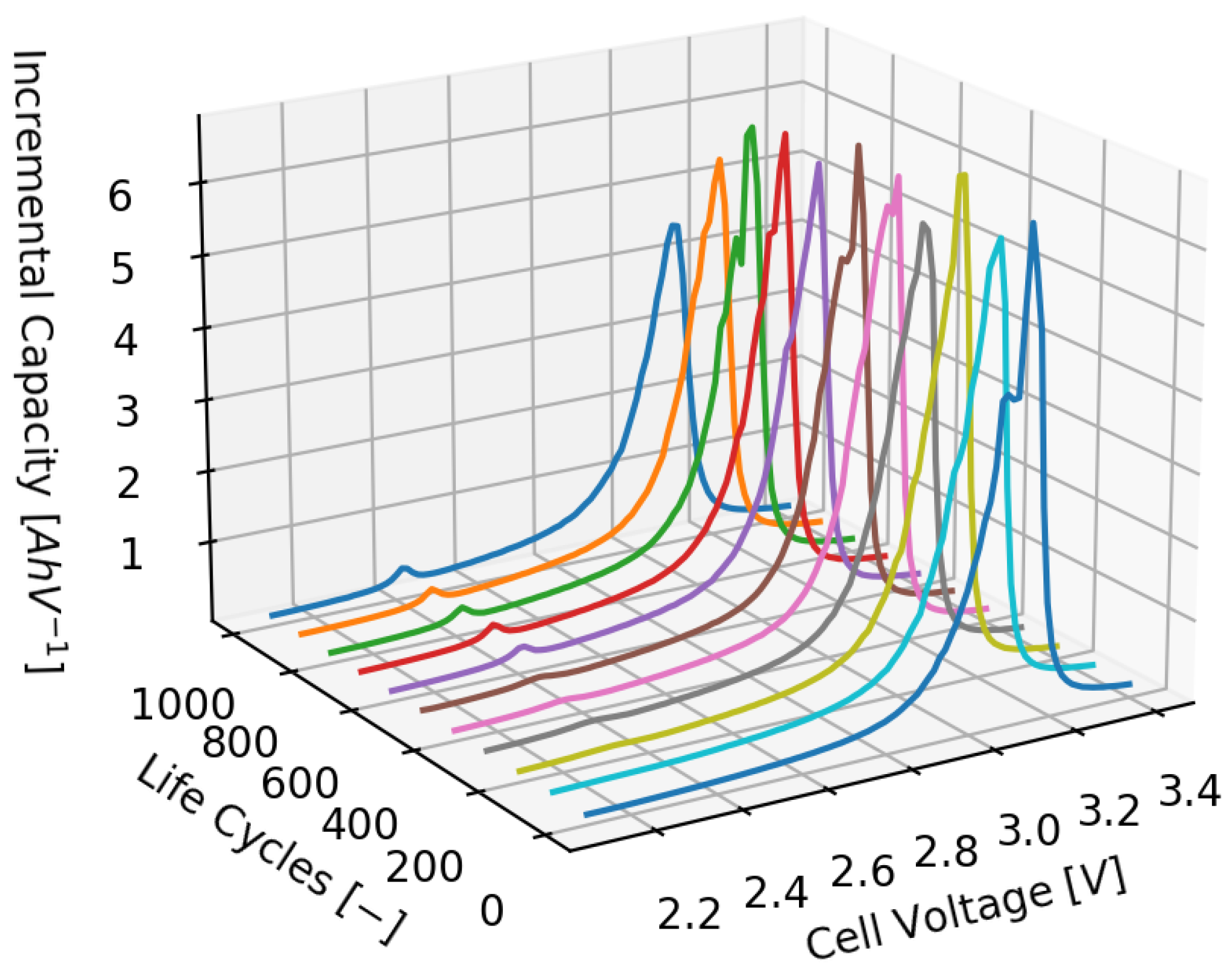
  23. Anseán, D.; González, M.; Blanco, C.; Viera, J.C.; Fernández, Y.; García, V.M. Lithium-ion battery degradation indicators via incremental capacity analysis. In Proceedings of the 2017 IEEE International Conference on Environment and Electrical Engineering and 2017 IEEE Industrial and Commercial Power Systems Europe (EEEIC/I&CPS Europe), Milan, Italy, 6–9 June 2017; pp. 1–6. [Google Scholar] [CrossRef]
  24. Severson, K.A.; Attia, P.M.; Jin, N.; Perkins, N.; Jiang, B.; Yang, Z.; Chen, M.H.; Aykol, M.; Herring, P.K.; Fraggedakis, D.; et al. Data-driven prediction of battery cycle life before capacity degradation. Nat. Energy 2019, 4, 383–391. [Google Scholar] [CrossRef] [Green Version]
  25. Benosman, M.; Atinç, G.M. Multi-parametric extremum seeking-based learning control for electromagnetic actuators. In Proceedings of the 2013 American Control Conference, Washington, DC, USA, 17–19 June 2013; pp. 1914–1919. [Google Scholar] [CrossRef]
  26. Benosman, M. Extremum Seeking-Based Indirect Adaptive Control and Feedback Gains Auto-Tuning for Nonlinear Systems. 2015. Available online: https://www.merl.com/publications/docs/TR2015-009.pdf (accessed on 7 November 2021).
Figure 1. Equivalent Circuit Models (ECM). (a) One Time Constant model. (b) Two Time Constants model. (c) Asymmetric OTC impedance model.
Energies 14 07496 g001
Figure 2. Incremental Capacity curves of a specific cell along its life.
Energies 14 07496 g002
Figure 3. Extremum seeking optimization scheme.
Energies 14 07496 g003
Figure 4. Optimization scheme.
Energies 14 07496 g004
Figure 5. Input current waveform.
Energies 14 07496 g005
Figure 6. Electrical parameter estimation results in the first scenario. (a) Cost function. (b) R S . (c) R P . (d) C P .
Energies 14 07496 g006
Figure 7. Voltage output in the first scenario.
Energies 14 07496 g007
Figure 8. Electrical parameter estimation results for the second scenario. (a) Cost function. (b) R S . (c) R P . (d) C P .
Energies 14 07496 g008
Figure 9. MRE evolution vs. cell aging. (a) R S . (b) R P . (c) C P .
Energies 14 07496 g009
Table 1. Electrical parameters of the ground truth model.
ParameterValueUnit
R S 60m Ω
R P 20m Ω
C P 4000F
Table 2. Error metrics for the first scenario.
ParameterErrorUnitMetric
R S 0.28%MRE
R P 0.78%MRE
C P 0.82%MRE
Voltage0.1mVRMSE
Table 3. Error metrics for the second scenario.
ParameterErrorUnitMetric
R S 0.34%MRE
R P 3.13%MRE
C P 0.9%MRE
Voltage0.2mVRMSE
Table 4. Error metrics for the third scenario.
ParameterErrorUnitMetric
R S 1.6%MRE
R P 79.5%MRE
C P 0.32%MRE
Voltage5.2mVRMSE
Publisher’s Note: MDPI stays neutral with regard to jurisdictional claims in published maps and institutional affiliations.

