1. Introduction and Motivation
In recent years, the main focal point of the automotive industry has shifted towards the development of autonomous vehicles. This challenge involves several problems, which must be solved before launching the first fully automated vehicle, e.g., decision making, accurate sensing and the design of robust and reliable control systems. During the last few decades, numerous control algorithms have been developed for the control and analysis of nonlinear and safety-critical systems, such as autonomous vehicles. Most of these control solutions are ordered as conventional control approaches and non-conventional learning-based control algorithms.
The classical approaches include the robust optimal methods (
) [
1], optimal controls (LQR,
) [
2], model predictive control (MPC) approaches [
3] and polytopic system-based algorithms (LPV) [
4]. The main advantage of these algorithms is that the achieved stability and performances of the closed-loop system can be analytically proven, at least for a specific region of their operating range. Furthermore, these solutions are good at handling the specific nonlinearities of the production plant and can also deal with unmodelled dynamics and noises as well. However, their performances can significantly degrade with the consideration of more uncertainties due to the resulting conservativeness of the worst-case approaches. Furthermore, the determination and description of the unmodelled dynamics and nonlinearities can also be a challenging task, which can make the control design difficult.
With the increasing computational capacity of computers and with the increased numbers of data sources, novel methods have become available for controlling autonomous vehicles, e.g., learning-based approaches. This group of methods can include algorithms, such as support vector machine (SVM) approaches [
5], or further learning methods with neural-network-based agents (e.g., supervised learning for achieving deep neural networks, reinforcement learning-based methods [
6], etc.). These algorithms have a significant advantage over the classical approaches: they use (and learn from) data, which describes the behavior of the control plant more accurately than any modeling process is capable of. Therefore, the performances of these solutions can be significantly better than classical approaches. However, most of the machine learning-based control algorithms have a notable pitfall, i.e., theoretical guarantees on the stability and performances of the closed-loop system cannot be provided.
Therefore, the engineers started focusing on the development of mixed control algorithms, which take advantage of both groups. For example, the combination of the machine learning algorithm and Linear Parameter Varying (LPV) approach can be found in [
4,
7]. Meanwhile, paper [
8] presents an MPC-based solution, which is extended with a machine learning-based reachability set computation for trajectory tracking of autonomous vehicles. The use of linearization feedback can be a promising approach to deal with the nonlinearities of the plant. However, the design of that feedback controller can also be a challenging task using classical methods, but neural networks can provide satisfying results. Since the classical approaches are good at guaranteeing predefined performances in the case of linear systems and an appropriately linearized system can eliminate the effect of the nonlinearities and other unmodelled dynamics, it can ease the control design.
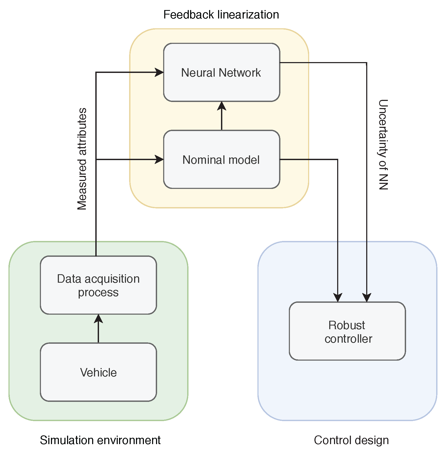
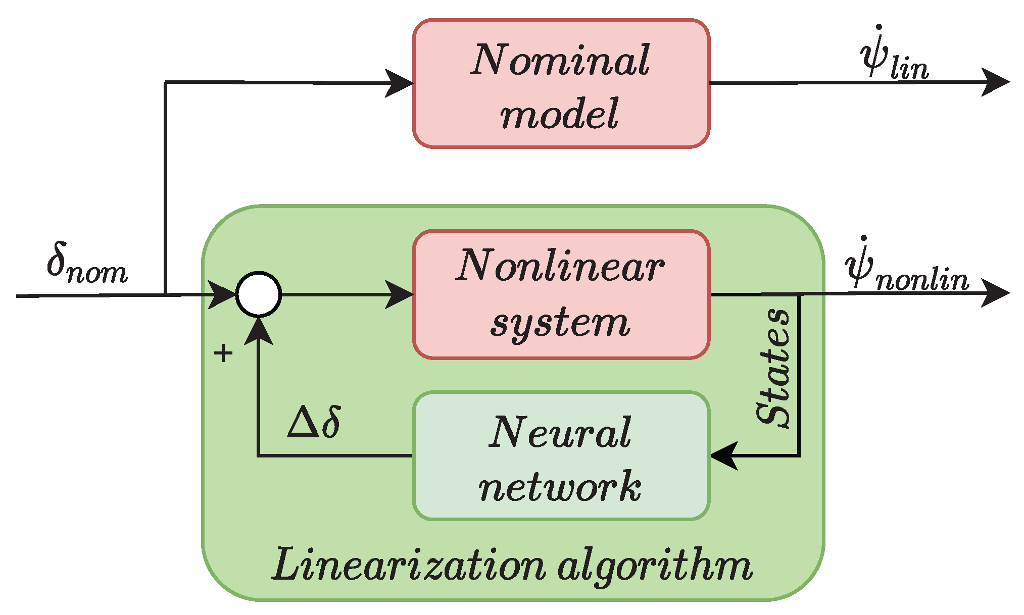
In this paper, a novel robust control algorithm is proposed, which exploits the advantages of both the classical control and machine-learning-based methods. The whole algorithm includes two main parts: the modeling and the control design phases.
Modeling phase: A neural network-based model matching is proposed, which aims to adjust the original nonlinear dynamics of the vehicle to a nominal, linear model.
Control design phase: A robust control design based on the method is presented, in which the fitting error of the resulting neural network is taken into account during the design phase.
The aim of the model-matching part is to eliminate the effects of the nonlinearities and uncertainties of the system. The neural network uses the measurable states of the vehicle and determines an additional steering angle. This means that the neural-network creates an inner loop of the control structure. Using the additional steering angle, the behavior of the vehicle is modified and the goal is to match it to the nominal model. The nominal model is determined using a classical single track dynamical bicycle model. The main challenge of using a neural network-based control algorithm is that the stability of the closed-loop system cannot be analytically proven. Therefore, a robust
controller is designed, which takes into account the effect and the errors of the neural network in order to compensate the mentioned pitfalls of the neural network. Briefly summarizing the contribution of the paper, the goal is to increase the performances and the stability of the closed-loop system by combining a machine learning-based model matching algorithm and a robust control approach. The main steps of the control design are illustrated in
Figure 1, and are:
- 1
Simulation environment, which provides the datasets for training the neural network.
- 2
Model-matching algorithm, which contains the training phase of the neural network.
- 3
Control design, in which the -based robust controller is designed.
The paper is structured as follows.
Section 2 presents the nominal vehicle model, which is used in the training of the neural network and in the robust control design phase as well.
Section 3 details the neural network-based model-matching method. The
-based lateral control design is presented in
Section 4. Finally, in the last section, a complex simulation example is given to show the operation and effectiveness of the proposed control algorithm.
2. Formulation of the Nominal Model
In this section, the formulation of the nominal model is presented. The aim of the formulation is to define the requested dynamics of the plant, which is achieved with the neural-network. Then, the formulated linear model is used as a plant for the control design.
The formulated model consists of two main parts: the lateral motion model, which is based on the two-wheeled bicycle model and the model of the steering system. Finally, the formulated model for data acquisition purposes is introduced.
2.1. Formulation of the Lateral Vehicle Model
The main idea behind the modeling method is to replace the front and rear wheels of the vehicle by one-one wheel, which are placed on the axis of symmetry of the vehicle. Basically, it consists of two equations: the first describes the lateral motion of the car, while the second equation represents its yaw-motion [
9]. The model is extended with an additional equation, which describes the connection between the lateral acceleration (
) and side-slip angle (
):
where
m is the mass of the car,
are geometrical parameters and
denotes the yaw-inertia. Moreover,
is the side-slip angle. The longitudinal velocity of the vehicle is (
), the steering angle is denoted by
and
is the yaw-rate. The lateral tire forces can be computed as:
where
is the cornering stiffness of the tires and
represents the side-slip angles of the tires. Using Equations (
1a,
1b,
1c) and (
2), a transfer function (
) can be determined. The input of the system is the steering angle
and the output is the yaw-rate (
) of the vehicle. This results in the following transfer function, which is formed as:
2.2. Dynamics of the Steering System
The presented model does not contain the dynamics of the steering system, which has a significant effect on the dynamics of the vehicle. Therefore, in the following, the model formulation of the steering system is detailed. The steering system can be effectively approximated by a second-order system [
10]:
where
and
are the parameters of the given system, which are determined through the identification process. During the identification process of the model parameters in (
4) the ARX (AutoRegressive model with eXogenous variable) structure is used, which is formed as:
where
y is the output of the system, which is the road-wheel angle (
) and the input of the system is the angle of the steering wheel. Using a
shift operator, the polynomials for
and
are the following:
The transfer function for the steering system can be formed as:
The details of the identification process (i.e., data acquisition, optimization method) behind the parameter selection was found in an earlier paper, see [
10].
2.3. Computation of the Inverse Model
Since the goal of the linearization process is to match the output of the real vehicle to the output of the nominal model, the computation of the input of the nominal model is required. It can be computed by using the inverse of the nominal model, which can be determined as [
11]:
However, the computation of the inverse model may result in a non-causal system, therefore a prefilter is applied to solve this issue.
where
denotes the transfer function of the prefilter. In the next step, the computed inverse of the transfer function is discretized using Tustin’s method [
12].
Finally, the presented inverse model () is used in the training of the neural network, which is presented in the following.
3. Neural Network-Based Model-Matching Algorithm
In this section, the neural network-based model matching algorithm is presented. The main purpose of this step is to modify the dynamics of the nonlinear system through an additional input signal. More precisely, the final goal of the model matching process is to achieve the same yaw-rate value of the nonlinear system as computed from the nominal model. In
Figure 2 the structure of the model matching process is shown. Basically, the neural network forms an internal loop in the control algorithm.
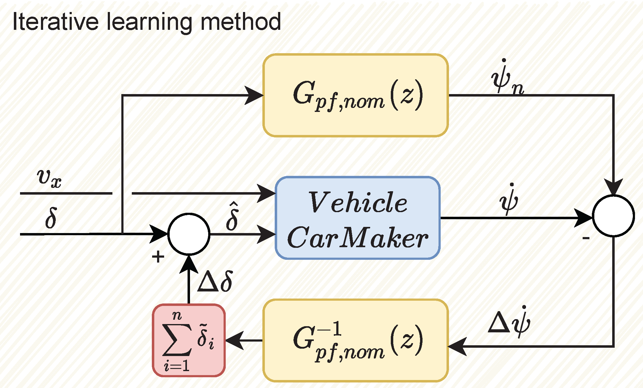
Since the real system is not accurately known, the computation of the additional control input is a challenging task. The whole system can be influenced by nonlinearities (e.g., tire characteristics) and uncertainties (e.g., velocity). This means, that the additional control input for the nonlinear model cannot be computed in only one step. In order to address this issue, an iterative algorithm is proposed, by which the additional control input can be determined for a predefined control input sequence. The main drawback of this algorithm is that it cannot be used in real-time applications. Therefore, a neural network is trained by using the results of the iterative algorithm, which can be used to determine the additional input signal during the operation of the control system. In the following, the generation of the training data is presented, which includes the computation of the additional steering angle .
3.1. Generation of the Training Data
In this paper, the CarMaker’s vehicle model is used as the nonlinear model, which is a complex, highly nonlinear vehicle model [
13]. As mentioned before, the determination of the additional steering angle cannot be determined in one step due to several uncertainties and nonlinearities. The main idea is to generate a reference input signal
sequence and a reference longitudinal velocity, which covers the whole operation range of the vehicle. Using the nominal model, and the generated input, the goal is to determine an additional steering angle sequence, by which the deviation between the computed yaw-rate (from the nominal model) and the measured yaw-rate (from the CarMaker) can be decreased. The steering angle and the longitudinal velocity vary in a wide range (
rad,
m/s). The structure of the iterative algorithm can be seen in
Figure 3.
The main goal of the iteration process is to calculate an additional steering angle sequence . The nominal yaw-rate () can be computed using the nominal model and the steering angle sequence. In each iteration step, the yaw-rate of the vehicle is measured and saved from CarMaker. The error between the two signals is computed and an additional steering angle is determined using the inverse of the nominal model.
In the first step of the iteration process, the input of the nonlinear system is the same as the input of the nominal model (
). Note that during the iterative process the reference control input sequence is not changed, this means that the nominal yaw-rate also remains the same. After computing the error between the two yaw-rate values, the additional steering angle (
) is determined using the inverse of the nominal model. This steering angle sequence is added to the nominal steering angle sequence and the simulation is performed using the modified sequence. After each iteration step, the additional steering angle is added to the previously determined steering angle sequence, as:
where
i denotes the
ith iteration step. Using the computed additional steering angle sequence the input for the nonlinear system can be determined as:
where
n gives the maximum number of iterations. Due to the differences between the nonlinear and the nominal model, the yaw-rate values may not match perfectly even after numerous iteration steps. In parallel, the use of a large number of iterations makes the whole process very time consuming. In order to solve this issue, the iterations continue until the highest error value becomes less then a previously defined value:
where
is a design parameter, and defines the maximum deviation between the output of the linear and the nonlinear model. In
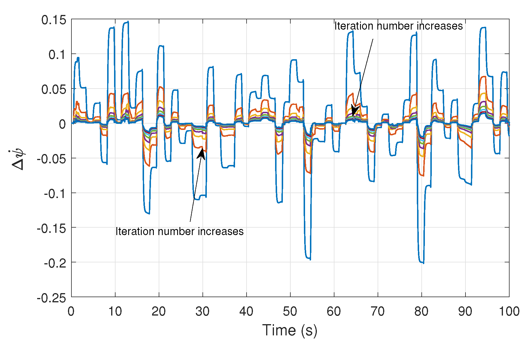
Figure 4 an example is presented for the iteration process.
As
Figure 4 illustrates, the error between the two outputs converges to zero. This means that using the computed additional steering angle sequence, nearly the same yaw-rate value can be achieved in case of the nonlinear system. Since the iterative algorithm cannot be used in real-time applications, a neural network is trained to determine the additional control input. The input of the neural network is the measurable states of the vehicle, which is saved at the last iteration step. The sampling time during the data collection was set to
s and over 200,000 data points were saved. For the training process of the neural network, the following attributes were saved and collected:
Longitudinal velocity ();
Accelerations (longitudinal , lateral );
Angular velocities (yaw-rate , pitch-rate , roll-rate );
Steering angle ();
The additional steering angle ().
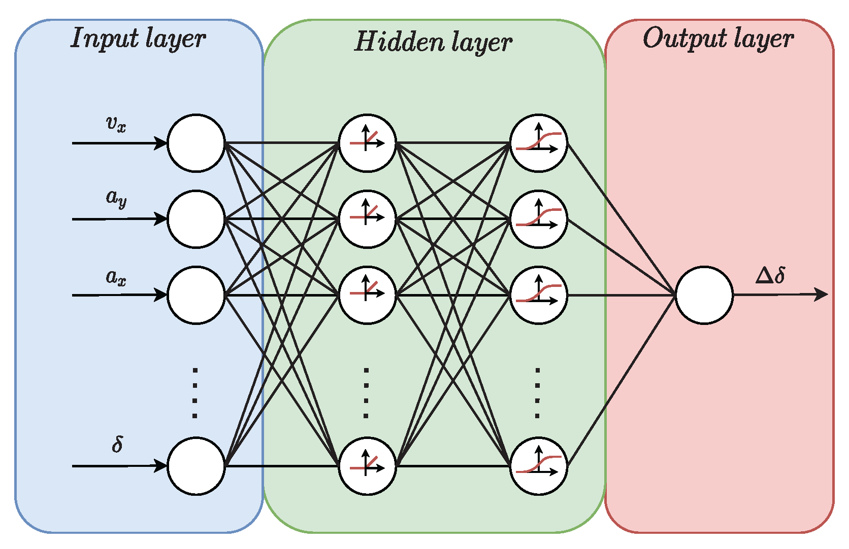
3.2. Training of the Neural Network
In this subsection, the training process of the neural network is presented. The basis of the training process is the collected dataset. The input vector of the network consists of the velocities, accelerations, angular velocities and the steering angle of the vehicle. The output of the network is the additional steering angle, by which the model matching is provided.
In general, the neural networks consist of three main types of layers: the input layer, the hidden layer, and finally the output layer. The layers are built up by weights and activation functions, and these functions are called neurons. Before the training process of the neural networks, the number of hidden layers and the activation functions must be chosen, see [
14]. The applied neural network consists of one input, one output, and two hidden layers. Since, the number of neurons can be chosen freely, to determine the optimal number of them, the so-called k-cross validation technique was used. The basic idea behind the k-cross validation technique is to divide the dataset into two subsets. The first one is used in the training process and the second one is for validation purposes. Moreover, in order to increase the generalization capability of the network, an additional Gaussian noise was added to the training dataset [
15]. In this case, the numbers of neurons in the hidden layers were chosen to 20 and 15. In the first hidden layer we used the rectified linear unit (ReLU), while in the second layer the log-sigmoid function was used. The training of the neural network was performed by a Levenberg-Marquardt algorithm, see [
14]. In
Table 1 the parameters, which are used for the training of the neural-network are summarized. The inputs of the neural network are the measurable data states of the vehicle, and the output is the computed additional steering angle (
). Using the computed additional steering angle, the model matching process is carried out.
In
Figure 5 the structure of the neural network is presented.
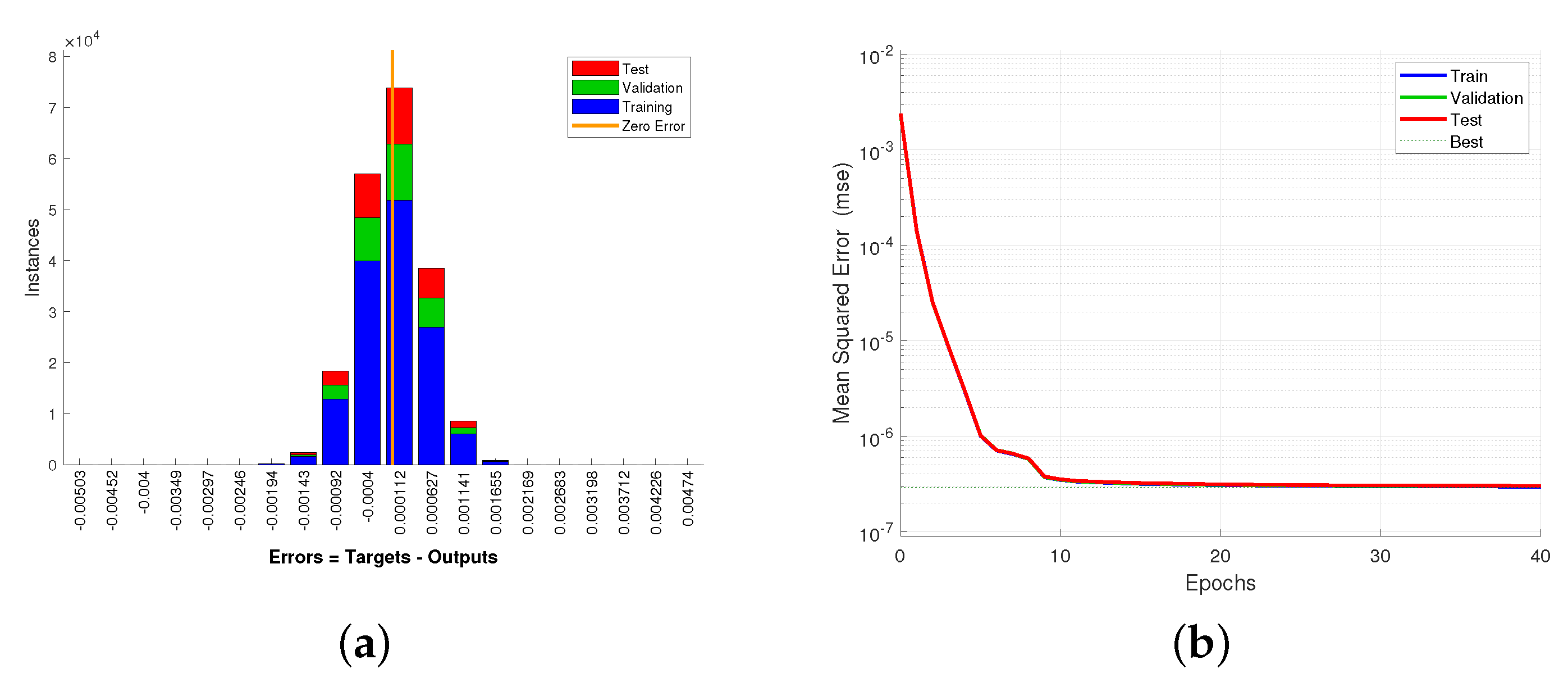
The results of the training process are shown in
Figure 6. The first figure shows error of the trained neural network, and the second figure presents the mean squared error during the training process.
In
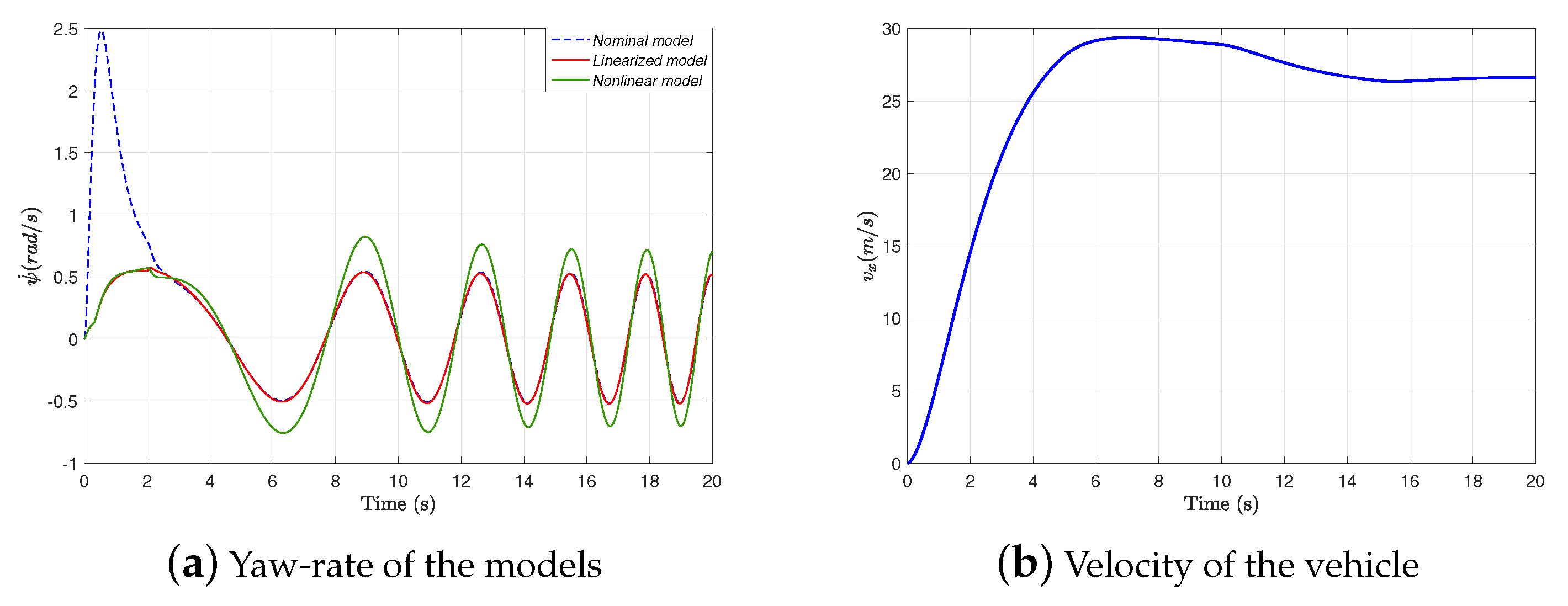
Figure 7 an example is presented, which shows the efficiency of the neural network. In this example, the neural network computes the additional steering angle, which is added to the nominal control input. Note that the data collection process used a step function-like input sequence (see:
Figure 4). Nevertheless, during this test the control input was selected for a different type of signal, which is a chirp signal. Using this different input signal, the generalization capability of the network was also examined.
During the test of the neural network, both the nonlinear and linear vehicle models are excited by the same chirp signal as the input of the system. As the figures show, the outputs of the linear nominal model (dashed blue line) and the linearized model (red line) are the same, apart from a short segment. At the beginning of the simulation, the velocity of the vehicle starts from zero, which causes significant inaccuracy in the linearization, since the presented nominal vehicle model is not valid at low longitudinal velocities. However, in other cases, the neural network provides satisfying results.
4. Robust Tracking Control Design Based on the Linearized Model
The linearized system is controlled by a
-based robust controller, whose design is detailed in this section. Since the neural network is able to linearize the plant, more precisely to fit the original nonlinear dynamics of the vehicle to the nominal model, the basis of the control design is the nominal model presented in
Section 2.
Although the resulted linearized system is able to approximate the requested linear system, error between the nominal and linearized models can be observed. Its reason is the error of fitting in the neural-network generation process. The error in the control design process as an uncertainty is taken into account. First, the modeling of the uncertainty is proposed and second, the design of the robust controller.
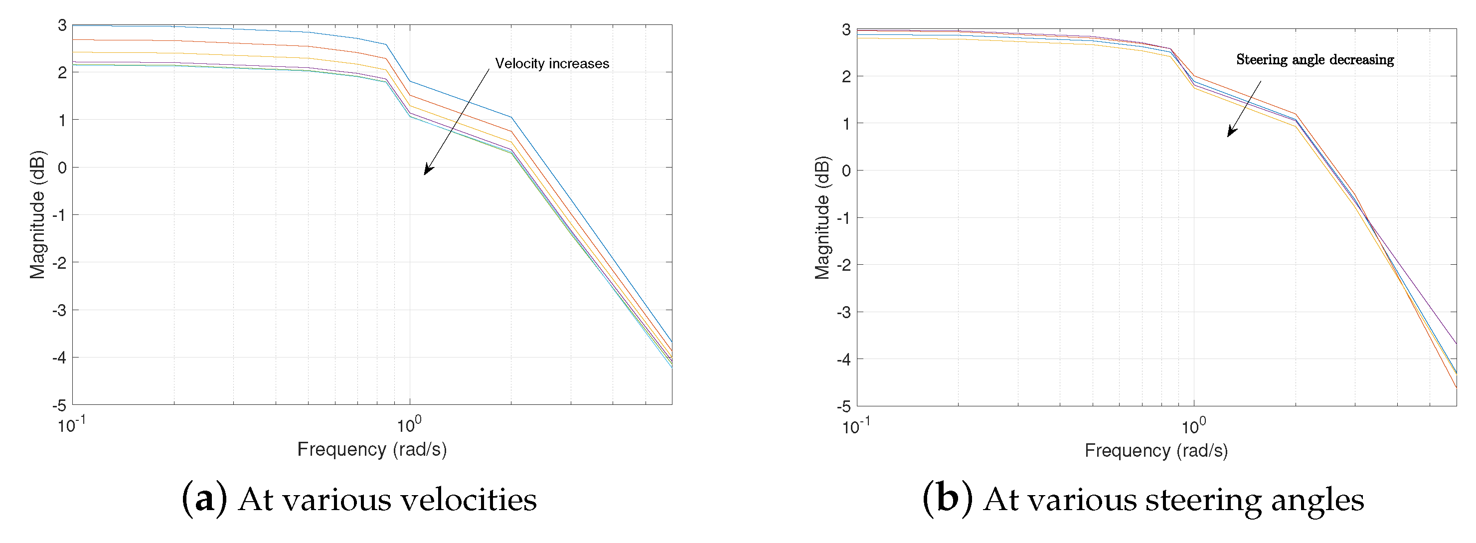
4.1. Uncertainty of the Linearized System
In order to quantify
, several simulations have been performed using the nonlinear vehicle model, which is implemented in CarMaker. During the simulations, the linearized system is excited with different steering angles (its amplitude
and frequency
, and the vehicle runs at different longitudinal velocities (
). Using the results of the simulations, each point of the transfer function from the measured yaw-rate (
) to the yaw-rate error (
) are calculated. The resulted transfer functions from the numerical computations are illustrated in
Figure 8.
As can be seen, the amplitude of the yaw-rate error () decreases along with the velocity and amplitude of the steering angle. The error of the neural network is handled as an uncertainty in the control design, which is described by the presented transfer functions.
The uncertainty of the system is formed through the worst-case scenario of the simulations. Thus, the uncertainty for the robust control design with the achieved highest magnitude of all scenarios is considered. The uncertainty from the difference between
and
is modeled as a first-order proportional term, i.e.,
where
are parameters, which are selected based on the simulation scenarios. Hence,
are fitted through a least-squares method to over-approximate the simulation results.
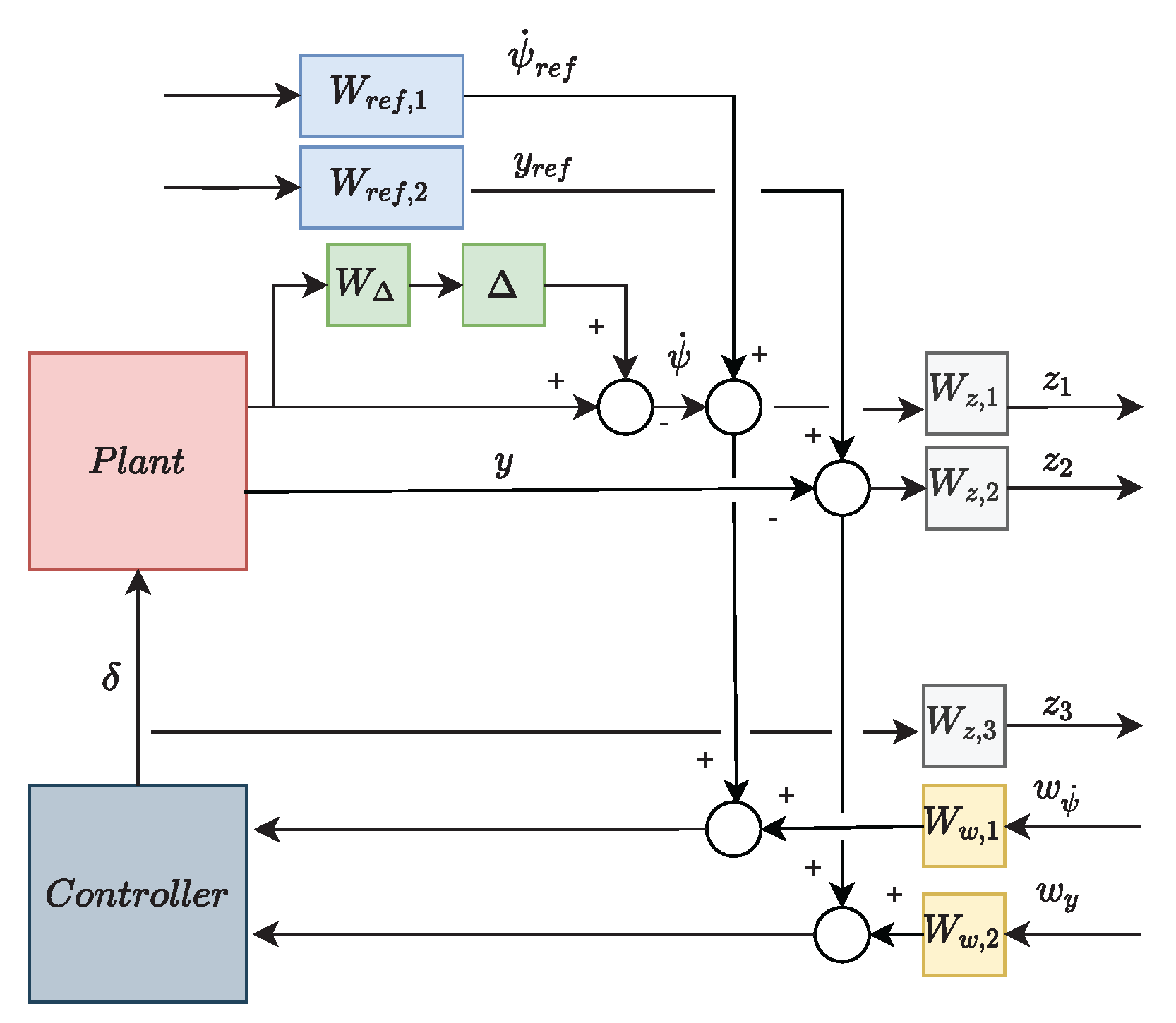
4.2. -Based Lateral Control Design
The main goal of the lateral control design is to guarantee the trajectory tracking of the vehicle, which can be achieved by the following performances:
The minimization of the lateral position:
In order to guarantee smooth trajectory tracking, the tracking of the reference yaw-rate is also prescribed:
The presented performances must be reached by using minimized intervention:
The performances can be written into the following vector:
. The state-space representation of the extended system:
where
A,
B and
are the matrices of the state-space representation of the nominal model (
1a,
1b,
1c), and its state vector:
.
is defined by the performances.
Figure 9 illustrates the augmented plant for the robust control design.
As can be seen, the plant is augmented with several weighting functions. The goal of the transfer functions
,
and
is to guarantee the predefined performances (
15)–(
17).
and
are to attenuate the noises of the measured signals (
,
y). The weighting functions
and
aim to scale the reference signals of the controller. Finally,
symbolizes the uncertainty of the neural network, which is determined from the presented simulations (
Figure 8).
The goal of the
design is to minimize the
-norm of the co-sensitivity functions of the closed-loop system (
), see [
16,
17]. This means that a
K controller must be found, which meets the following criterion:
Moreover, the resulted controller (
K) must also guarantee that the closed-loop system is asymptotically stable. Finally,
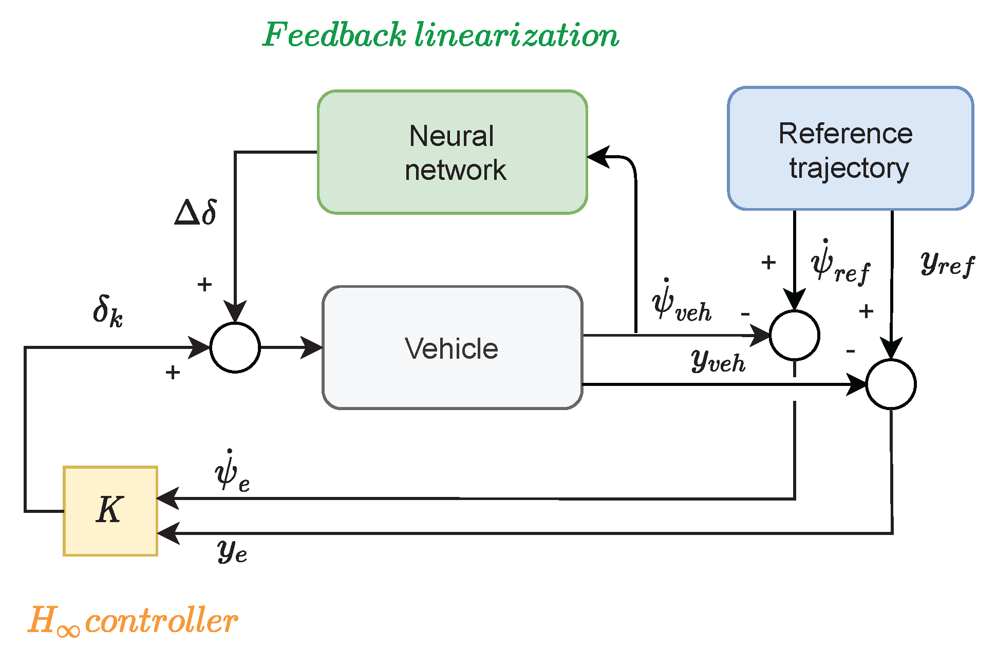
Figure 10 shows the whole control algorithm including the neural network-based model-matching method.
5. Simulation Example
A comprehensive simulation is presented in this section, which is made using CarMaker vehicle dynamics simulation software. During the simulation, the goal is to track the given reference trajectory at varying longitudinal velocities, which contains sharp bends, where the vehicle is close to its physical limits. The car is driven along the given section of the track twice. In the first case, the vehicle is controlled by the extended robust controller (with the neural network-based linearization), while in the second case, it is driven by the plain nominal robust controller.
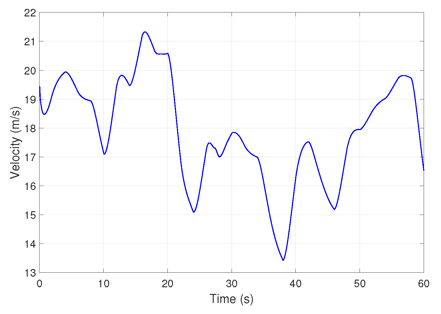
Figure 11 shows the longitudinal velocity profile of the vehicle. The velocity varies in a high range between
{13–22 m/s}.
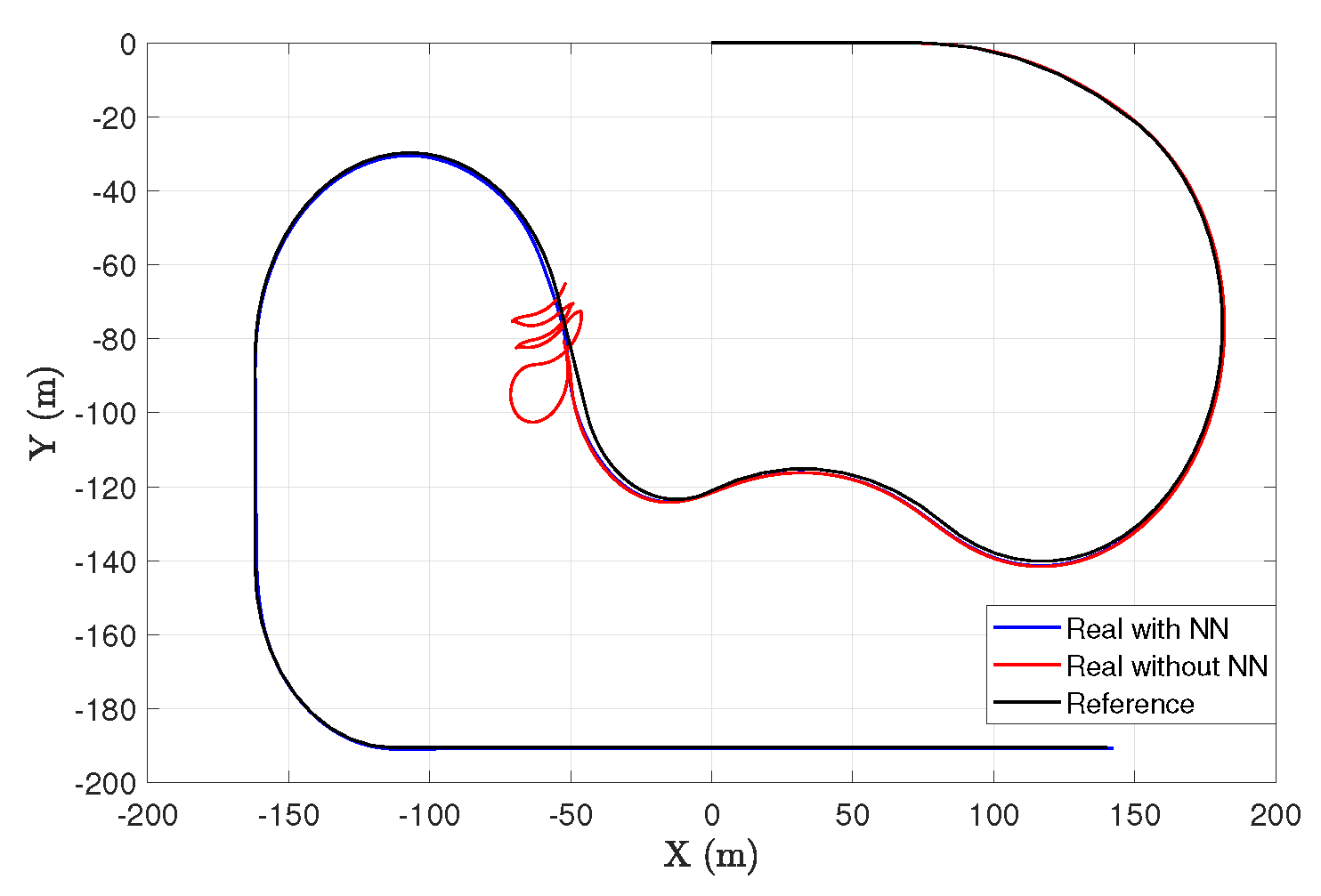
Figure 12 demonstrates the trajectory tracking of the vehicle for both cases. In the first case, when the car is driven by the extended controller, it is able to follow the predefined track. In the other case, the vehicle leaves the road at a sharp bend. It means that the nominal controller is not able to guarantee the required performance.
Figure 13 depicts the lateral acceleration of the vehicle using the extended controller. As can be seen, the lateral acceleration varies between
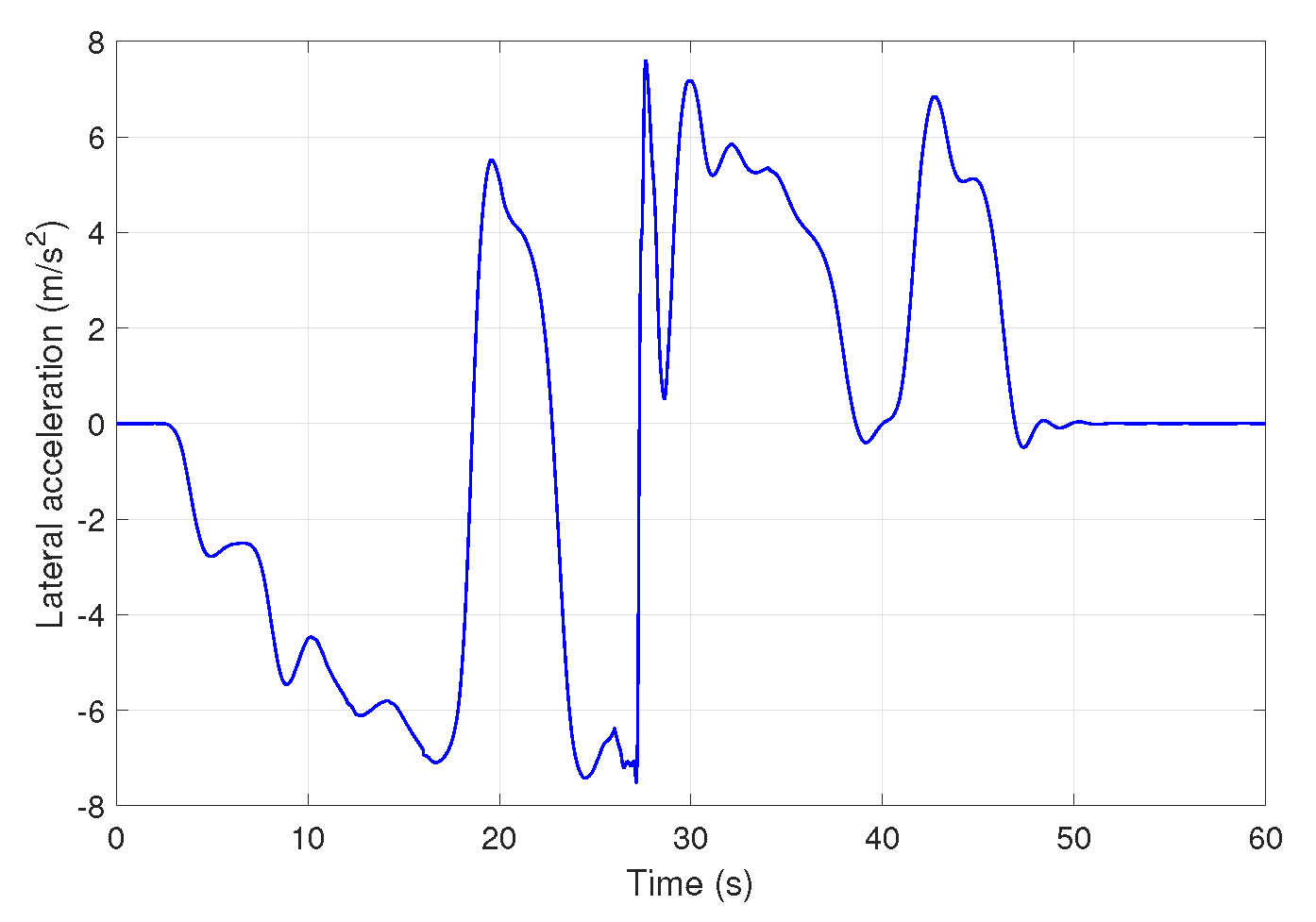
, 8 m/s
}, which means it is close to the physical limits of the car. Basically, this is the cause of the unstable behavior of the vehicle in the second case, when the nominal controller is used.
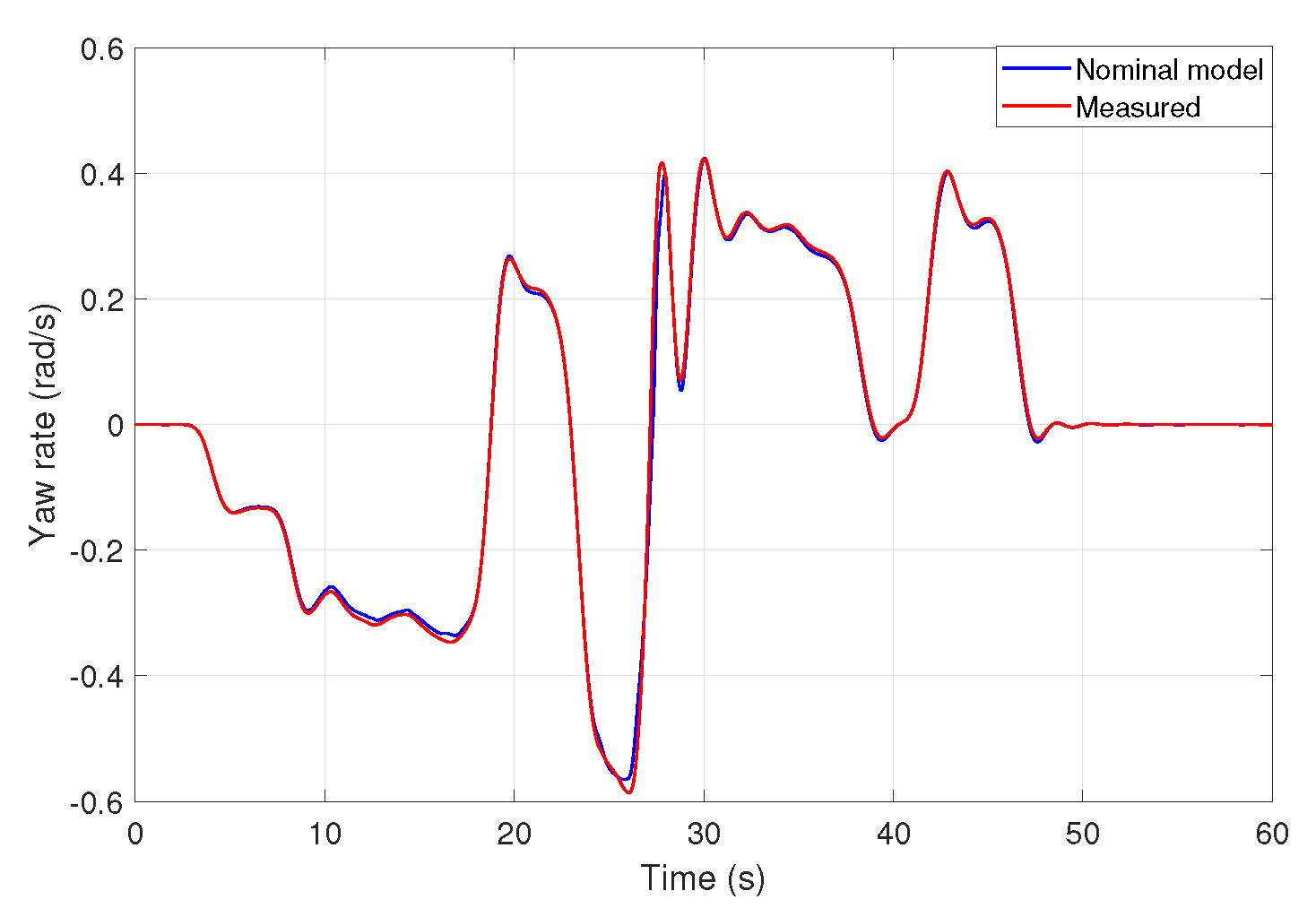
Figure 14 presents the yaw-rates of the vehicle. The yaw-rate of the nominal model is denoted by the blue line, while the measured yaw-rate is given by the red line. As the figure shows, the yaw-rate signals are close to each other, which means the linearization algorithm provides satisfying performances.
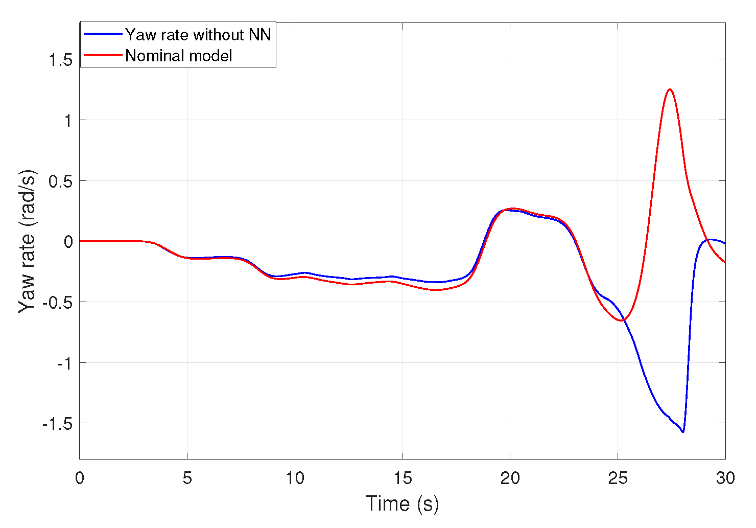
Figure 15 demonstrates the yaw-rate for the case when the neural network-based model-matching is not used. It can be seen that the two signals differ from each other, especially at the sharp bend, where the vehicle becomes unstable.
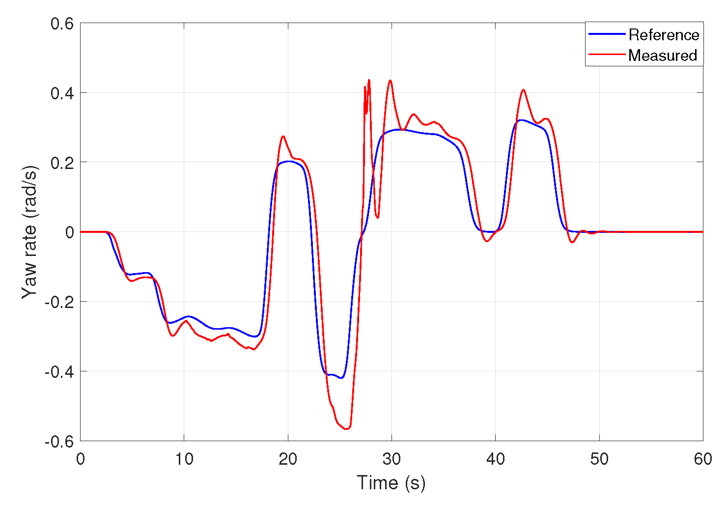
The reference and the measured yaw-rate signals are illustrated in
Figure 16. The error of the tracking has a maximum of
rad/s. This value may be considered to be high; however, a balance must be found between the tracking of the lateral position and the yaw-rate, which is dealt with by weighting functions illustrated in
Figure 9.
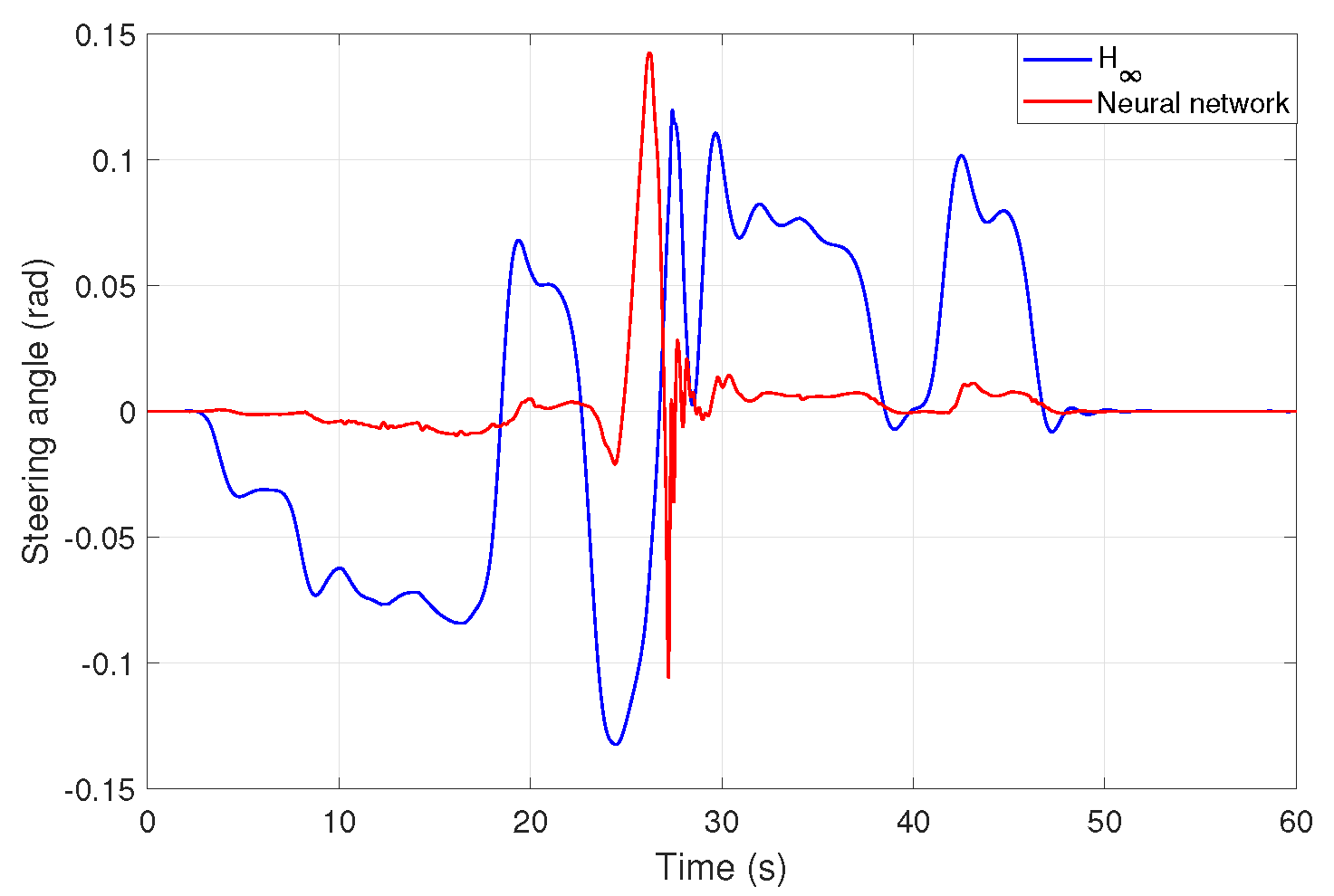
Finally, in
Figure 17 the input signals are shown. It can be seen that the neural network intervenes significantly when the vehicle is traveling at high velocity at the sharp bend. Whilst, in other cases, when the vehicle is in the linear range, the neural network provides a significantly smaller steering angle.
It can be concluded that the extended controller can ensure the stability requirements, especially in those cases, when the vehicle is close to its physical limits. Moreover, the performance of the model-matching algorithm has been investigated in [
18].
6. Conclusions
In this paper, a novel -based robust control algorithm has been proposed for autonomous vehicles, which was extended with a neural network-based model-matching approach. The main role of the neural network is to match the output of the nonlinear system to the predefined linear one. The error of the neural network has also been taken into account during the design phase as uncertainty on the measured signal. Finally, a complex simulation example has been given, which showed the advantage of the proposed control algorithm over the nominal robust controller. The whole simulation is performed in a vehicle dynamics simulation software, CarMaker.
Author Contributions
Conceptualization, algorithms, software, T.H. and D.F.; methodology, T.H., D.F. and B.N.; supervision, P.G. All authors have read and agreed to the published version of the manuscript.
Funding
The research was supported by the Ministry of Innovation and Technology NRDI Office within the framework of the Autonomous Systems National Laboratory Program. The research was partially supported by the National Research, Development and Innovation Office (NKFIH) under OTKA Grant Agreement No. K 135512. The work of Tamás Hegedus and Dániel Fényes have been supported by the ÚNKP-21-3 New National Excellence Program of the Ministry for Innovation and Technology from the source of the National Research, Development and Innovation Fund.
Institutional Review Board Statement
Not applicable.
Informed Consent Statement
Not applicable.
Data Availability Statement
No data available.
Conflicts of Interest
The authors declare no conflict of interest.
References
- Wang, R.; Jing, H.; Hu, C.; Yan, F.; Chen, N. Robust H8 Path Following Control for Autonomous Ground Vehicles with Delay and Data Dropouts. IEEE Trans. Intell. Transp. Syst. 2016, 17, 2042–2050. [Google Scholar] [CrossRef]
- Yakub, F.; Mori, Y. Comparative study of autonomous path-following vehicle control via model predictive control and linear quadratic control. Proc. Inst. Mech. Eng. Part D J. Automob. Eng. 2015, 229, 1695–1714. [Google Scholar] [CrossRef]
- Németh, B.; Hegedus, T.; Gaspar, P. Model Predictive Control Design for Overtaking Maneuvers for Multi-Vehicle Scenarios. In Proceedings of the 2019 18th European Control Conference (ECC), Naples, Italy, 25–28 June 2019; pp. 744–749. [Google Scholar]
- Fenyes, D.; Nemeth, B.; Gaspar, P. LPV-based autonomous vehicle control using the results of big data analysis on lateral dynamics. In Proceedings of the 2020 American Control Conference (ACC), Denver, CO, USA, 1–3 July 2020; pp. 2250–2255. [Google Scholar]
- Xu, F.; Qu, Y.; Qu, T.; Chen, H.; Liang, D. Support Vector Machine Based Model Predictive Control for Vehicle Path Tracking Control. In Proceedings of the 2020 39th Chinese Control Conference (CCC), Shenyang, China, 27–29 July 2020; pp. 2461–2466. [Google Scholar]
- Ji, X.; He, X.; Hen, L.; Liu, Y.; Wu, J. Adaptive-neural-network-based robust lateral motion control for autonomous vehicle at driving limits. Control Eng. Pract. 2018, 76, 41–53. [Google Scholar] [CrossRef]
- Balázs, N.; Gáspár, P. Ensuring performance requirements for semiactive suspension with nonconventional control systems via robust linear parameter varying framework. Int. J. Robust Nonlinear Control 2020, 31, 8165–8182. [Google Scholar] [CrossRef]
- Fenyes, D.; Nemeth, B.; Gaspar, P. Impact of big data on the design of MPC control for autonomous vehicles. In Proceedings of the 2019 18th European Control Conference (ECC), Naples, Italy, 25–28 June 2019; pp. 4154–4159. [Google Scholar]
- Rajamani, R. Vehicle Dynamics and Control; Springer: Berlin/Heidelberg, Germany, 2005. [Google Scholar]
- Hegedus, T.; Fenyes, D.; Nemeth, B.; Gaspar, P. Handling of tire pressure variation in autonomous vehicles: An integrated estimation and control design approach. In Proceedings of the 2020 American Control Conference (ACC), Denver, CO, USA, 1–3 July 2020; 2244–2249. [Google Scholar]
- Shamash, Y. Construction of the inverse of linear time-invariant multivariable systems. Int. J. Syst. Sci. 1975, 6, 733–740. [Google Scholar] [CrossRef]
- Malinen, J. Tustin’s method for final state approximation of conservative dynamical systems. IFAC Proc. Vol. 2011, 44, 4564–4569. [Google Scholar] [CrossRef]
- IPG Automotive. CarMaker 9.2. Available online: https://ipg-automotive.com/products-services/simulation-software/carmaker (accessed on 27 October 2021).
- Demut, H.; Hagan, M.; Beale, M. Neural Network Design; PWS Publishing Co.: Boston, MA, USA, 1997. [Google Scholar]
- Li, Y.; Liu, F. Whiteout: Gaussian Adaptive Noise Regularization in Deep Neural Networks. arXiv 2016, arXiv:1612.01490. [Google Scholar]
- Scherer, C.; Weiland, S. Lecture Notes DISC Course on Linear Matrix Inequalities in Control; Delft University of Technology: Delft, The Netherlands, 2000. [Google Scholar]
- Boyd, S.; Ghaoui, L.E.; Feron, E.; Balakrishnan, V. Linear Matrix Inequalities in System and Control Theory; Society for Industrial and Applied Mathematics: Philadelphia, PA, USA, 1997. [Google Scholar]
- Hegedus, T.; Fenyes, D.; Nemeth, B.; Gaspar, P. Improving Sustainable Safe Transport via Automated Vehicle Control with Closed-Loop Matching. Sustainability 2021, 13, 11264. [Google Scholar] [CrossRef]
| Publisher’s Note: MDPI stays neutral with regard to jurisdictional claims in published maps and institutional affiliations. |
© 2021 by the authors. Licensee MDPI, Basel, Switzerland. This article is an open access article distributed under the terms and conditions of the Creative Commons Attribution (CC BY) license (https://creativecommons.org/licenses/by/4.0/).


