Network Cost Estimation for Mini-Grids in Large-Scale Rural Electrification Planning

Abstract

Universal access to electricity is a crucial challenge in many developing countries. Establishing the electrification agenda of an underserved region is a complicated task where computer models play a critical role in calculating geospatial plans that efficiently allocate resources. Such plans should include—among other things—reasonable estimations of the designs and economic costs of standalone systems, mini-grids, and grid extensions. This implies that computer models need to estimate the network cost for many potential mini-grids. To that end, most planning tools apply quick rules of thumb or geometric methods that ignore power flows and electric constraints, which play a significant role in network designs. This paper presents a methodology that rapidly estimates any low-voltage mini-grid network cost without neglecting the impact of electrical feasibility in such cost. We present a case study where we evaluate our method in terms of accuracy and computation time. We also compare our method with a quick estimation similar to the ones most regional planning tools apply, showing the effectiveness of our method.

1. Introduction

Around 759 million people do not have access to electricity [1], and significant efforts are imperative to achieve universal access to energy in 2030 [2]. Moving towards this goal implies dealing with complex electrification planning where regulatory, financial, political, and techno-economic factors interact [3]. Even if we only consider the techno-economic perspective, a robust analysis requires computational tools that help the decision-maker in the planning process.

Electrification plans involve deciding which areas should be electrified with off-grid solutions and where grid extensions are the most economical alternative. In addition, these plans should estimate technical generation designs for off-grid systems and network layouts for mini-grids and grid extensions, providing an approximated budget for the material and components included in the designs.

Accurate cost estimations are crucial in planning as they provide a robust foundation for the elaboration of plans. One essential cost is related to distribution networks of mini-grids and grid extensions. According to reference [4], the cost of distribution networks, metering elements and end-user devices of several mini-grids located in sub-Saharan Africa is 21% of their total cost (on average). Similarly, reference [5] shows that the distribution costs account for 14% of the total CAPEX (on average) for 53 mini-grids in developing countries.

Several large-scale electrification planning models have been developed over the past few years [6], and they can be classified according to their modeling complexity [7]. A high modeling complexity generally involves substantial data and long computation times to calculate the recommended plan, but it leads to precise cost estimations and detailed designs.

Some models take advantage of Geographical Information Systems (GIS), providing instant access to geospatial data. They generally divide the consumers into cells and estimate the levelized cost of electricity (LCOE) of several alternatives to determine the recommended electrification solution of each cell. The models in this category usually estimate the network costs with analytical expressions or simple rules of thumb, providing fast solutions at the expense of reduced modeling detail. The Open Source Spatial Electrification Tool (OnSSET) [8,9] and IntiGIS [10,11] are representative models of this methodology.

Other planning models operate with villages or settlements, and calculate the network layout of the grid extension with methods based on geometrical features. Network Planner [12] works with villages, and applies an iterative approach based on the Kruskal algorithm to calculate the network layout of the villages electrified with grid extensions. GEOSIM also works with villages, clustering them among Development Poles (i.e., villages that are considered particularly important according to several criteria) [13,14]. However, these models also apply simplified methods to estimate the network cost of mini-grids.

The Reference Electrification Model (REM) operates with a very high level of modeling detail. REM works with individual consumers instead of villages or cells, and calculates detailed network designs that go down to the building level for grid extensions and mini-grids [15]. The model also obtains precise generation designs for mini-grids and standalone systems [16]. The optimization procedure that REM applies to obtain the network layouts considers the usual electric constraints and power flows (among other factors), but its iterative application to all the potential mini-grids and grid-extensions in large-scale planning is computationally expensive.

Other methods and tools calculate network designs for a single off-grid system. Village Power Optimization model for Renewables (ViPOR) calculates the network of a mini-grid applying a simulated annealing algorithm [17]. Reference [18] presents a method that calculates the network layout of a mini-grid in the context of rural electrification. However, the scope of these methods is limited, and it is unclear if they could be directly applied at a large scale—where the network cost of potentially thousands of mini-grids is calculated to elaborate an electrification plan.

Therefore, the current methods that estimate the network costs of mini-grids in the literature are oversimplified (which is the case of most regional planning tools), require a significant amount of computation time (which is the case of REM), or it is unclear if they could be applied in large-scale planning (which is the case of ViPOR and the remaining village-based tools for network designs).

As network costs play a significant role in electrification plans, it is worthwhile to develop a method that overcomes the limitations mentioned above by balancing accurate network cost estimations with quick calculations. The regional planning tools that apply oversimplified network cost estimations could greatly benefit from this method as their results would include realistic network costs, and REM could take advantage of this method to alleviate the computational burden related to high-level resolution planning.

This paper presents a methodology to estimate distribution network costs for mini-grids in large-scale planning. The method goes beyond the rules of thumb that most regional planning models apply. However, it avoids the computational burden of explicitly calculating the detailed layout of the network considering electric constraints and power flows (such as REM does). Instead, the method obtains a set of representative mini-grids and calculates detailed network designs for them alone. Then, it uses this information to estimate the cost of other designs rapidly and accurately.

The rest of this paper is structured as follows: Section 2 describes the relevant metrics regarding the network cost of mini-grids, and Section 3 presents the network cost estimation method. Section 4 introduces a case study, and the results of our method are compared with an estimation aligned with the methods of regional planning tools. Finally, Section 5 includes the conclusions as well as suggestions for future research.

2. Mini-Grid Metrics

This section describes the metrics that our method considers as potential drivers of the network cost. The metrics capture the electric and geometric properties that we expect to represent the network cost of a mini-grid. The method we present does not necessarily use all the metrics described in this section, but it selects the ones that are better estimators of the network cost for each case study.

Our method considers electric moments, which depend on the spatial distribution of consumers and their demands. It also considers spatial metrics relatively fast to calculate, such as the length of the minimum spanning tree (MST) that links all the consumers and the generation site in a mini-grid. Similar approaches are present in other fields in the literature. Moments have been successfully used for pattern recognition in diverse areas, such as image recognition [19,20], but they have also proven to be useful in power systems [19].

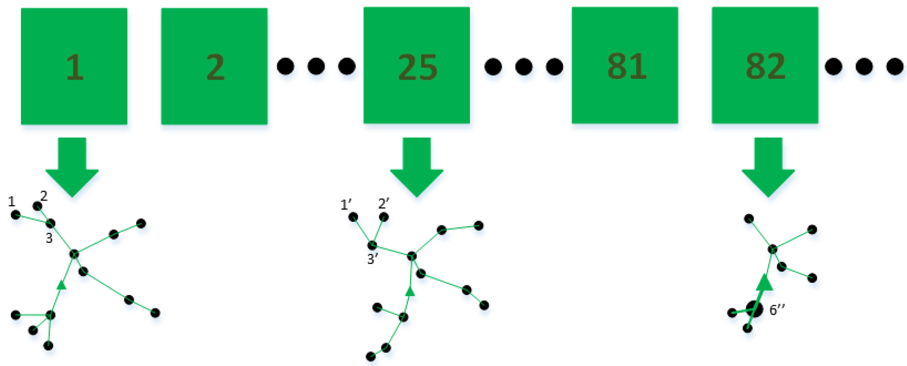
If several mini-grids are very similar in terms of consumers and demand, they could have similar network costs. Figure 1 provides an illustrative example, showing the distribution network of several mini-grids, which have been labeled 1, 25, and 82 in the example. Mini-grids 1 and 25 are equal in terms of the number of consumers, with thirteen consumers each. These mini-grids also have equal aggregated demands (we assume that the load profile of each consumer is proportional to its size in Figure 1, and therefore all the consumers have the same load profile in both mini-grids). Finally, the spatial distribution of consumers in mini-grids 1 and 25 is very similar (if we overlap the graphical representation of both networks, then consumer 1 would be very close to consumer 1’, consumer 2 would be very close to consumer 2’, and so on). Therefore, all these similarities (number of consumers, aggregated demands, and spatial distribution) imply that mini-grids 1 and 25 could have similar network costs.

On the contrary, mini-grid 82 is different from mini-grids 1 and 25. Mini-grid 82 has only eight consumers, and they are less scattered around its generation site than the consumers of mini-grids 1 and 25. Consequently, it seems that mini-grid 82 has lower network costs than networks 1 and 25, but mini-grid 82 has a productive consumer with a large demand (consumer 6”). This productive consumer may significantly increase the overall network cost of mini-grid 82, which could end up being similar to the network cost of mini-grids 1 and 25.

There is a clear correlation between several metrics of a mini-grid and its network cost. If we compare two mini-grids that are identical in every aspect but demand, then the one with the greater demand is expected to have a higher network cost. Similarly, if we account for the network cost of two mini-grids that only differ in the location of their consumers, then the one with more dispersed consumers is expected to be more expensive. Size and demand are, therefore, two important cost drivers that our method considers.

However, the network cost of a mini-grid does not change if we move all its consumers a certain distance or if we rotate them around a certain point. The following properties formalize these intuitive ideas about the metrics:

Cost-monotonicity: when the metric increases its value, the network cost also increases or stays at the same level.

Translation-invariance: the network cost of a mini-grid does not change if all the consumers of that mini-grid are translated a specific distance in the same direction.

Rotation-invariance: the network cost of a mini-grid does not change if all its consumers are rotated a specific angle around the same point.

Scale-monotonicity: If we scale a mini-grid so that its consumers are more dispersed, network cost will increase so the values of the metrics should also increase.

Table 1. Mini-grid metrics.

Type	Variable
Electric	Electric moments (central)
	Electric moments (rotation)
	Aggregated and peak demand
Spatial	Minimum-spanning-tree length
	Minimal area rectangle (min{width, height}, area, perimeter)
Other	Number of consumers

presents the metrics, which are described in Section 2.1, Section 2.2 and Section 2.3.

The metrics selected are fundamental as the results of our method depend on them. The remainder of this section provides some insights regarding why we have selected the metrics presented in Table 1.

The MST length is a crucial driver of the network cost of mini-grids as the MST attempts to obtain a least-cost design under purely geometrical considerations. Many regional planning tools estimate network cost by applying methods that rely on calculating an MST [7]. For example, Network Planner uses an iterative method based on an MST to determine which villages are electrified with the power grid and the layout of the corresponding grid extension [12]. Similarly, reference [20] uses a technique that aims at optimizing the topology of the power grid, and this technique starts by calculating the MST of a set of clusters.

Although the MST length provides vital information regarding the network costs, it lacks information regarding the size of the mini-grid. In that regard, we included several metrics of the Minimal Area Rectangle (MAR) to capture information concerning the area covered by the mini-grid.

Regarding the electric metrics, it is clear that demand plays a crucial role in electrification planning [15] and mini-grid design [21]. High demand levels lead to high distribution network costs and vice versa, so we included the aggregated and the peak demand of mini-grids in the list of metrics considered to capture the impact of demand on network costs.

Electric moments have been widely used as a dimensionality reduction tool in several fields of power systems, such as transmission expansion planning [19,22] and rural electrification [23]. Central moments are included because they capture a combination of the spatial location and the peak demands of the consumers of a mini-grid, which is an important piece of information regarding network costs. However, central moments change when mini-grids are rotated around a point (i.e., they are not rotation invariant), so we included the rotation moments too because they satisfy this property.

Finally, the number of consumers of a mini-grid is used as a quick approximation of the network cost in several applications. For example, Network Planner estimates low-voltage distribution costs multiplying the total number of consumers minus one by other parameters [24]. Moreover, some regional plans that calculate the cost of densification by grid extension assume that the network needed is directly proportional to the number of consumers [25]. Therefore, we included the number of consumers in the metrics that our method considers.

2.1. Electric Metrics

In this section, we briefly introduce the electric metrics that our method considers. These metrics include the electric central moments, the electric rotation moments, and the demand-related metrics.

2.1.1. Electric Moments (Central)

The $\left(p,q\right)$ central electric moment is defined by Equation (1):

$${\mu }_{p,q}=\iint {\left(x-\overline{x}\right)}^p{(y-\overline{y})}^{q}f\left(x,y\right)dxdy$$

(1)

where the integral limits are given by the boundaries of the mini-grid and $f\left(x,y\right)$ is the peak demand of the consumer $\left(x,y\right)$. In practice, we have a discrete number of consumers $c$ so the integral becomes a summation when computing the moments.

$${\mu }_{p,q}={\displaystyle \sum }_{i=1}^{i=c}{\left(x_i-\overline{x}\right)}^p{(y_i-\overline{y})}^{q}f\left(x_i,y_i\right)$$

(2)

The $\left(n+1\right)$ moments of order $n$ are given by the solutions of the equation $n=p+q$, being $p,q$nonnegative integers. The moments of odd order decrease when a consumer with negative coordinates $\left(-x,-y\right)$is included in a mini-grid. This causes undesired effects since there is no difference in the final network cost between adding a consumer with coordinates $\left(x,y\right)$ or $\left(-x,-y\right)$ to a symmetric (with respect to the origin of coordinates) mini-grid. Therefore, all moments of odd order and moments of even order where variables have an odd exponent do not satisfy the cost-monotonicity property, and we do not consider them useful predictor variables.

Hence, we include only the central moments of even orders where all the variables have even exponents. In practical terms, it is enough to include central moments of orders 2, 4, and 6. The inclusion of additional central moments does not tend to improve the accuracy of the models and generally produces collinearity among the variables.

References [26,27] show that the central moments are invariant to translation. If a mini-grid is scaled, then the distances between its consumers and the centroid of the mini-grid increase and the central moments included increase too, so the central moments included meet the scale-monotonicity property. Similarly, if one of the central moments included increases, then the demand rises or the distances between its consumers and its centroids increases, so the network cost should rise. Therefore, the central moments included meet all the properties described in this section except rotation invariance. The electric rotation moments are included to compensate for that.

2.1.2. Electric Moments (Rotation)

Reference [26] introduces the rotation moments for image recognition, and they are translation and rotation invariant.

$$I_1={\mu }_{2,0}+{\mu }_{0,2}$$

(3)

$$I_2={({\mu }_{2,0}-{\mu }_{0,2})}^2+4{\mu }_{1,1}^2$$

(4)

$$I_3={({\mu }_{3,0}-3{\mu }_{1,2})}^2+{(3{\mu }_{2,1}-{\mu }_{0,3})}^2$$

(5)

$$I_4={({\mu }_{3,0}+{\mu }_{1,2})}^2+{({\mu }_{2,1}+{\mu }_{0,3})}^2$$

(6)

$$\begin{gathered} I_5=({\mu }_{3,0}-3{\mu }_{1,2})({\mu }_{3,0}+{\mu }_{1,2})[{({\mu }_{3,0}+{\mu }_{1,2})}^2-3{({\mu }_{2,1}+{\mu }_{0,3})}^2]+(3{\mu }_{2,1} \\ -{\mu }_{0,3})({\mu }_{2,1}+{\mu }_{0,3})[3{({\mu }_{3,0}+{\mu }_{1,2})}^2-{({\mu }_{2,1}+{\mu }_{0,3})}^2] \end{gathered}$$

(7)

$$I_6=({\mu }_{2,0}-{\mu }_{0,2})[{({\mu }_{3,0}+{\mu }_{1,2})}^2-{({\mu }_{2,1}+{\mu }_{0,3})}^2]+4{\mu }_{1,1}({\mu }_{3,0}+{\mu }_{1,2})({\mu }_{2,1}+{\mu }_{0,3})$$

(8)

$$\begin{gathered} I_7=(3{\mu }_{1,2}-{\mu }_{3,0})({\mu }_{3,0}+{\mu }_{1,2})[{({\mu }_{3,0}+{\mu }_{1,2})}^2-3{({\mu }_{2,1}+{\mu }_{0,3})}^2] \\ +({\mu }_{0,3}-3{\mu }_{2,1})({\mu }_{2,1}+{\mu }_{0,3})[3{({\mu }_{3,0}+{\mu }_{1,2})}^2 \\ -{({\mu }_{2,1}+{\mu }_{0,3})}^2] \end{gathered}$$

(9)

Reference [28] highlights that these moments are do not form a complete or independent basis and adds another third-order rotation moment:

$$I_8={\mu }_{1,1}[{({\mu }_{3,0}+{\mu }_{1,2})}^2-{({\mu }_{0,3}+{\mu }_{2,1})}^2]-({\mu }_{2,0}-{\mu }_{0,2})({\mu }_{3,0}+{\mu }_{1,2})({\mu }_{0,3}+{\mu }_{2,1})$$

(10)

Since $I_1$ is a linear combination of electric central moments of order two we will not consider it as a candidate variable, and we will include the remaining rotation moments $I_2-I_8$.

2.1.3. Demand

Although the peak demands of individual consumers are already considered in the calculation of electric moments, the aggregated and peak demands of a mini-grid may provide valuable information, and they are included in the metrics considered. The demand-related metrics included meet all the properties described in this section.

2.2. Spatial Metrics

In this section, we briefly describe the spatial metrics that our method considers. These metrics include the MST length and several metrics related to the MAR.

2.2.1. Length of the MST

The length of the MST linking all consumers is calculated with the consumers of the mini-grid and the generation site located at the demand-weighted center of the mini-grid, which is an appropriate placement for the generation site (for example, REM always locates the generation site at this spot). This metric meets all the properties described in this section.

2.2.2. Minimal Area Rectangle

The MAR refers to the rectangle of minimum area that contains all the consumers of the mini-grid. The main geometric attributes of the minimum rectangle of a set of points (consumers) are rotation-invariant, translation-invariant, and scale-variant, meeting all the desirable properties we identified beforehand. Besides, any increase in these metrics should lead to a more substantial network cost. 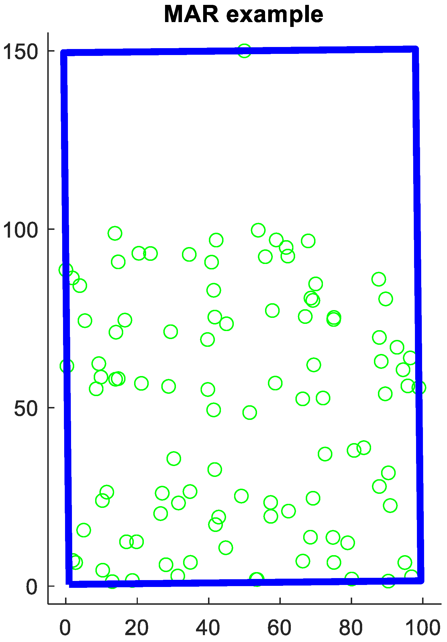Figure 2 shows an example with several points and their corresponding MAR.

MAR is sensitive to extreme values. The example provided in Figure 2 has one extreme value with coordinates (50, 150) that significantly increases the area and perimeter values. Since the perimeter depends linearly on the width and the height of the rectangle, the metrics considered include area, perimeter, and the minimum between its height and width.

2.3. Other Metrics

This section describes additional metrics that are useful to consider. For the time being, the only metric that belongs to this section is the number of consumers of the mini-grids.

2.3.1. Number of Consumers

We included several metrics that measure the “size” of a mini-grid (such as the length of the MST or the aggregated demand). The number of consumers of a mini-grid is an additional metric correlated to its size, and it is also considered. This metric meets all the properties described in this section.

3. Method

This section describes the method this paper proposes to estimate the network cost of mini-grids accurately and quickly. We should highlight that the method has two constraints or limitations. The first one is related to the voltage levels used in the distribution network: our method assumes that all mini-grids deploy an LV distribution network, which is consistent with the usual planning results. The second one is related to topography: our method also assumes that the topographical features of the terrain are not critical in the cost of the distribution network (i.e., for the time being, our method does not explicitly consider the impact of topography on the network cost).

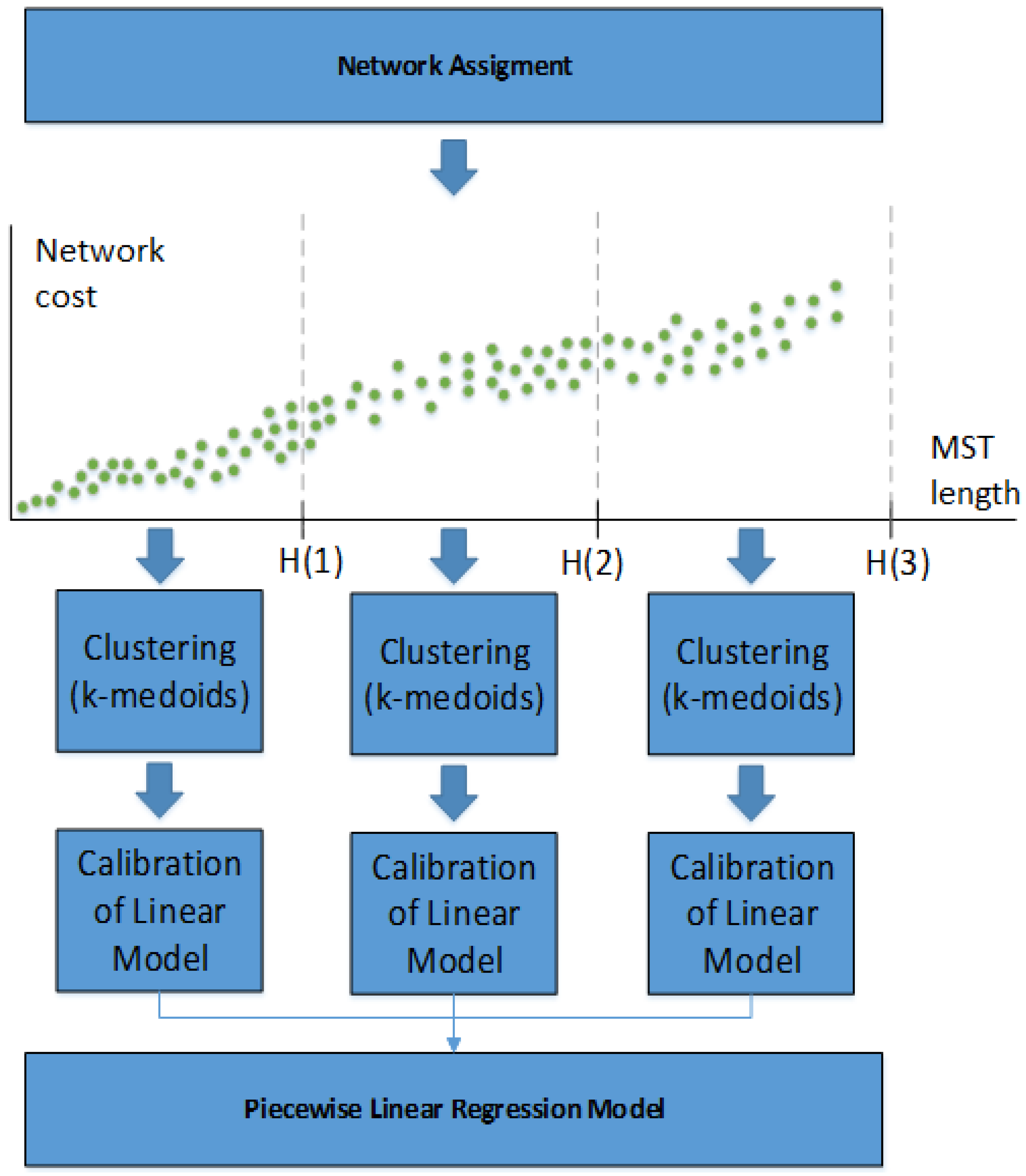
Figure 3 shows a flow chart of the method, which follows three sequential steps. The first step is network assignment, which calculates the number of linear regression models needed and assigns the mini-grids to the models (a data point represents each one). The second step is clustering, which applies a k-medoids algorithm to obtain a set of representative mini-grids for each linear regression model. The final step is the calibration of linear models, which calculates detailed network designs for the representative mini-grids, and determines the metrics and coefficients of the linear regression models.

Regression methods have already been used in the context of large-scale electrification planning to obtain accurate cost estimations within a reasonable computation time. Reference [29] uses a multivariate regression model to estimate the generation cost of mini-grids, showing that the cost error between using their method and a quick approximation on a rule of thumb is more than 10% on average for certain types of mini-grids. Similarly, reference [30] applies regression methods to calculate the generation cost of mini-grids as well as their installed capacities.

The application of these two regression methods follows a sequential process similar to the one shown in Figure 3: a set of representative mini-grids is obtained (which our method does in the clustering step), and accurate designs are calculated for these mini-grids. Then, a model is adjusted so that the costs of the remaining mini-grids can be quickly obtained without optimizing the corresponding designs from scratch (which our method does in the calibration of linear models step).

However, our method includes an additional step at the beginning that is missing in references [29,30], which is the network assignment and it distributes the mini-grids to the models. This step is necessary because our method uses several linear regression models instead of a single one. One advantage of using several linear models to estimate the network cost of the mini-grids is that our method can select different metrics and coefficients for each linear model.

For example, a linear model with small mini-grids that supply only residential consumers could consider only the length of the MST of the mini-grids to estimate their network cost accurately. However, another linear model that estimates the network cost of large mini-grids that include productive loads could also include several electric metrics to capture the impact of productive loads and provide accurate estimations of the network costs.

Even if the metrics of several linear models are the same, their coefficients will be different, and the cost estimation will be better than the one obtained with a single linear model. The rest of this section describes our method in detail.

3.1. Network Assignment: Determination of the Number of Models to Fit and Their Correspondence with Particular Mini-Grids

The network assignment step determines the number of linear regression models to use, and it distributes all mini-grids of the case study among the models. The use of several linear regression models and the classification of the whole analysis dataset among them (i.e., piecewise linear regression) has been applied to capture trends in multiple fields in the literature, such as suicide rates [31,32], cancer mortality rates [33,34], population structural changes [35], and the impact of traffic policies [36].

However, the main goal of network assignment is to avoid assigning mini-grids whose network costs have different orders of magnitude to the same model. Therefore, we developed a tailored method to distribute the mini-grids among the linear models. In our method, two mini-grids are assigned to the same linear model if and only if their network costs are of the same order of magnitude. One way of achieving this is to ensure that the quotient between the lengths of the MSTs of any pair of mini-grids that belong to the same model is lower than or equal to a threshold $Q$. Equation (11) forces this constraint for each model $n\in \left\{1, 2,\dots , N\right\}$:

$$\frac{\mathit{max}\left(length\left(MS{T}_n\right)\right)}{\mathit{min}\left(length\left(MS{T}_n\right)\right)}\le Q$$

(11)

where $MS{T}_n$ refers to the MSTs of the networks assigned to the $n-th$ model. The total number of models $N$ depends on each case and must be calculated. Let $u$ and $U$ be the minimum and maximum lengths of all the MSTs (in km), respectively. We consider the sequence:

$$\left\{u,Q·u,Q^2·u,\dots ,Q^{N-1}·u,Q^N·u\right\}$$

(12)

It is clear that the quotient between any pair of consecutive terms in the sequence is equal to $Q$, so $N$ linear models are necessary and sufficient. —if Equation (13) holds and $N$ is the minimum natural number that satisfies Equation (13), then we have $u<Q·u<Q^2·u<\dots <Q^{N-1}·u<U\le Q^N·u$ and we could group the mini-grids in $N$ linear models whose MST lengths lie in the ranges $\left[u,Q·u\right)$, $\left[Q·u,Q^2·u\right)$,…,$\left[Q^{N-1}·u,Q^N·u\right]$. Similarly, if Equation (13) does not hold we would need at least $N+1$ linear models to group all the mini-grids ensuring that Equation (11) is satisfied—as long as $N$ is the minimum natural number that satisfies Equation (13):

$$U\le Q^N·u$$

(13)

Dividing both sides by $u$ and taking logarithms yields:

$$lo{g}_Q\left(U/u\right)=lo{g}_Q\left(U\right)-lo{g}_Q\left(u\right)\le N$$

(14)

So Equation (15) provides the minimum number of linear models needed in terms of $U, u$ and $Q$.

$$N=lo{g}_Q\left(U\right)-lo{g}_Q\left(u\right)$$

(15)

where $\lceil x\rceil$ is the lowest integer that is greater than or equal to $x$. However, Equation (15) implies that the number of models tends to infinity if $u$ tends to zero, so Equation (15) is only applied if $u\ge 1/Q$ to avoid potential issue. Otherwise, the number of models is determined considering that a linear model could cover the range of MST lengths $\left[u,1\right]$, and $N-1$ models could cover the range $\left[1, U\right]$. Equation (15) is applied to the range $\left[1, U\right]$ to determine $N-1$, which yields:

$$N=lo{g}_Q\left(U\right)-lo{g}_Q\left(1\right)+1=lo{g}_Q\left(U\right)+1$$

(16)

Equation (16) is also valid if $1/Q<U\le 1$ because in that case only one model is needed to cover the range $\left[u,U\right]\subset \left[u,1\right]$, and $\lceil lo{g}_Q\left(U\right)\rceil =0$ so $N$ is set to the correct value. If $U\le 1/Q$, then $N$ is directly set to 1. Equation (17) comprises all the expressions used to calculate $N$ in terms of $U, u$ and $Q$.

$$N=\{\begin{array}{c}\lceil lo{g}_Q\left(U\right)-lo{g}_Q\left(u\right)\rceil if U>u\ge 1/Q \\ \lceil lo{g}_Q\left(U\right)\rceil +1 if U>1/Q>u \\ 1 if 1/Q\ge U>u\end{array}$$

(17)

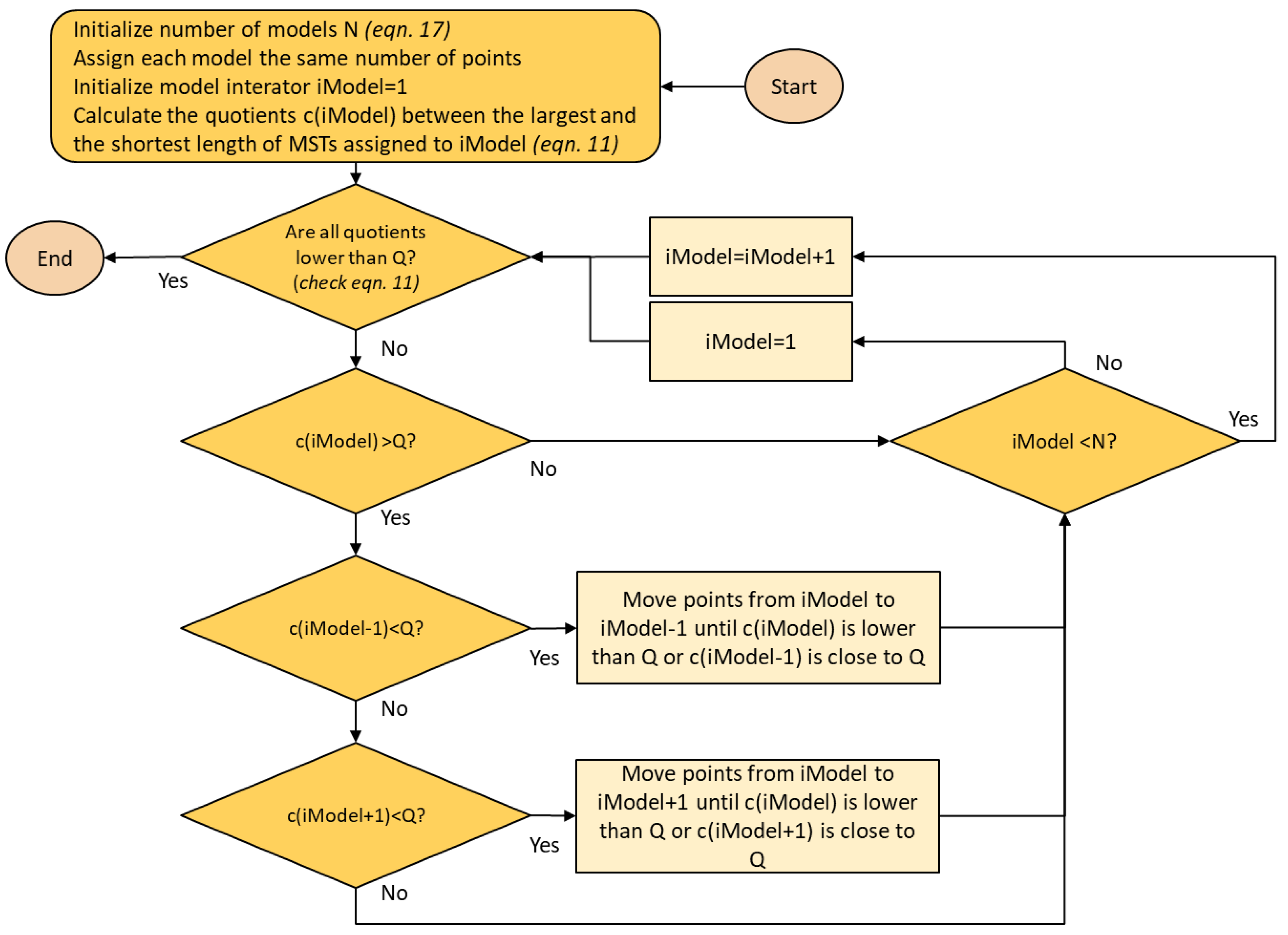
Once the number of models has been determined, the mini-grids are distributed among the linear models. This process initializes each model with the same number of mini-grids. It calculates the quotients between the maximum and minimum lengths of MSTs for each model and, for those models that do not satisfy Equation (11), it reassigns mini-grids from the closest models (if they meet Equation (11)) to reduce their quotient. This process goes on iteratively until Equation (11) holds for each model (the first model may not be forced to satisfy this equation if $u<1/Q<U$). Figure 4 shows a stylized flow diagram of the network assignment.

The threshold $Q$ is set to ten in the case study [37], although other values are possible because Equation (11) implicitly assumes that there is a perfect linear correlation between the MST and the network cost, which is not true (although the correlation is usually very high). Setting $Q$ to a value slightly lower than ten could mitigate the impact of this assumption because the maximum cost difference among the mini-grids that belong to the same linear model would be reduced.

3.2. Clustering (K-Medoids)

Once the algorithm has assigned the mini-grids to linear models, the clustering step obtains a representative set of mini-grids for each linear model. Detailed network designs are calculated later for representative mini-grids, so the clustering outcome should be real mini-grids that exist in the case study. To that end, the clustering step applies a k-medoids algorithm, which also turns out to be more robust to outliers than other methods such as k-means [38].

There are several implementations of the k-medoids algorithm in the literature. The Partitioning Around Medoids (PAM) calculates an initial solution, and then performs all possible swaps among medoids and non-medoids to improve the solution [39]. The main drawback of PAM is that it is a computationally-intensive process that does not perform well when dealing with large datasets. Clustering for LARge Applications (CLARA) tries to overcome this drawback by applying PAM only on a reduced sample of the original dataset, trading optimality for computation speed. The Clustering LARge Applications based on RANdomized Search (CLARANS) also samples only a part of the original dataset, but the sample is not selected beforehand [40].

Our method applies the Matlab build-in function to perform the k-medoids algorithm [41], which uses the PAM algorithm if input points are lower than 3000. If the input points are between 3000 and 10,000, then it applies a method based on reference [42]. If the number of input points is larger than 10,000, then it evaluates a subset of the data following a procedure similar to CLARANS.

K-medoids is applied several times with an increasing number of clusters, and the sums of point-to-medoid distances are computed. The process stops when the marginal gain of increasing the number of clusters drops below a pre-established threshold [43].

The clustering step always considers the length of the MST (a representative spatial metric) and the aggregated demand (a representative electric metric) to determine the representative mini-grids. These two metrics are scaled since they are measured with different units. The length of the MST is scaled with the average cost of the LV lines of the catalog, which is a reasonable estimation of how much the network cost would increase for a given increment of the MST length. The aggregated demand is scaled by an estimation of the network cost per kWh in the analysis region, which could be obtained by expert advice or looking at previous reports or publications that deal with electrification planning projects in the corresponding region.

3.3. Calibration of Linear Models

This step calculates accurate network designs for the representative mini-grids, which are calculated using the Reference Network Model (RNM) [44]. RNM designs distribution networks considering power flows to ensure the feasibility of the networks. This model operates with a network catalog that includes several line capacities for each voltage level and several transformer sizes, and it can handle topographical elements such as altitudes and penalized areas.

RNM was initially designed to help the regulator estimate distribution network cost and establish a fair remuneration for the operation, maintenance and expansion of the distribution network in developed regions. REM applies RNM to calculate accurate network designs for mini-grid and grid extensions, showing that RNM can be used in the context of rural electrification (such as we do in this paper). Reference [45] gives further details on the interaction between REM and RNM.

Once our method has calculated accurate distribution networks for the representative mini-grids, the “Calibration of linear models” step determines the most representative metrics for each model and their coefficients applying hierarchical regression [46]. This technique has been successfully applied in many fields [47,48].

Hierarchical regression starts with an initial linear model and adds blocks of variables sequentially. The process continues until the addition of variables does not improve the model, or there are no more variables to add. The hierarchical levels determine the order followed to include variables in the model: the first hierarchical level corresponds to the initial linear model, the second level contains the first block of variables added to the model, and so on.

The expertise of the analyst plays a critical role in hierarchical regression, as he or she needs to determine which variables are assigned to each hierarchical level. The most relevant variables should be included in the initial levels, and the less important ones should be incorporated in later stages.

We also considered applying stepwise regression, which is a similar procedure that starts with an initial linear model, and variables are introduced or removed sequentially. In stepwise regression, the sequential order of variables is determined by their statistical significance (i.e., the computer determines the order by calculating p-values).

Results are hard to replicate with stepwise regression, as small variations in the dataset could lead to different regression models [49]. This would be a significant issue since we are obtaining our representative networks with a k-medoids algorithm (whose outcome may depend on the initial solution).

Table 2. Models used in the hierarchical regression.

Hierarchical Level	Variables Added
1	Length of the MST
2	Number of consumers
3	Central moments of order 2
4	Central moments of order 4
5	Central moments of order 6
6	Minimum area rectangle metrics
7	Demand
8	Rotation moments

shows the variables included in each hierarchical level (a hierarchical level also includes all the variables of the previous levels). The initial level also includes a constant term.

We consider the MST length the most relevant variable, followed by the number of consumers and its central moments grouped by their order. This way, levels 1–5 include the spatial, electric, and “other” metrics that we consider paramount. Levels 6–8 include the remaining metrics.

To avoid collinearity, our method applies the Belsley collinearity test [50] and removes the collinear variables from their corresponding hierarchical level. We also compute the p-values to check at which point it is not worth adding more variables to the model.

4. Case Study

This section presents an application to a case study located in Rwanda, comparing the exact network cost of mini-grids with the approximation that our method provides. The location of the consumers and their demand profiles are based on the case presented in [51]. The location of residential consumers was obtained by combining information from the HRSL [52], a report from SOFRECO [53], and the expected population growth for 2024 [54]. Energy Development Corporation Limited (EDCL) provided the location of the productive loads.

The shape of the hourly demand profile of the loads was estimated according to in-the-field surveys conducted in the village of Gicumbi [55,56]. The peak demands of the residential consumers are based on the high-demand case shown in [15], whereas the peak demands of the remaining loads are based on [51].

The network catalog is based on the experience of the Universal Access Laboratory, which is based on their participation in several projects combined with field trips and conducted interviews.

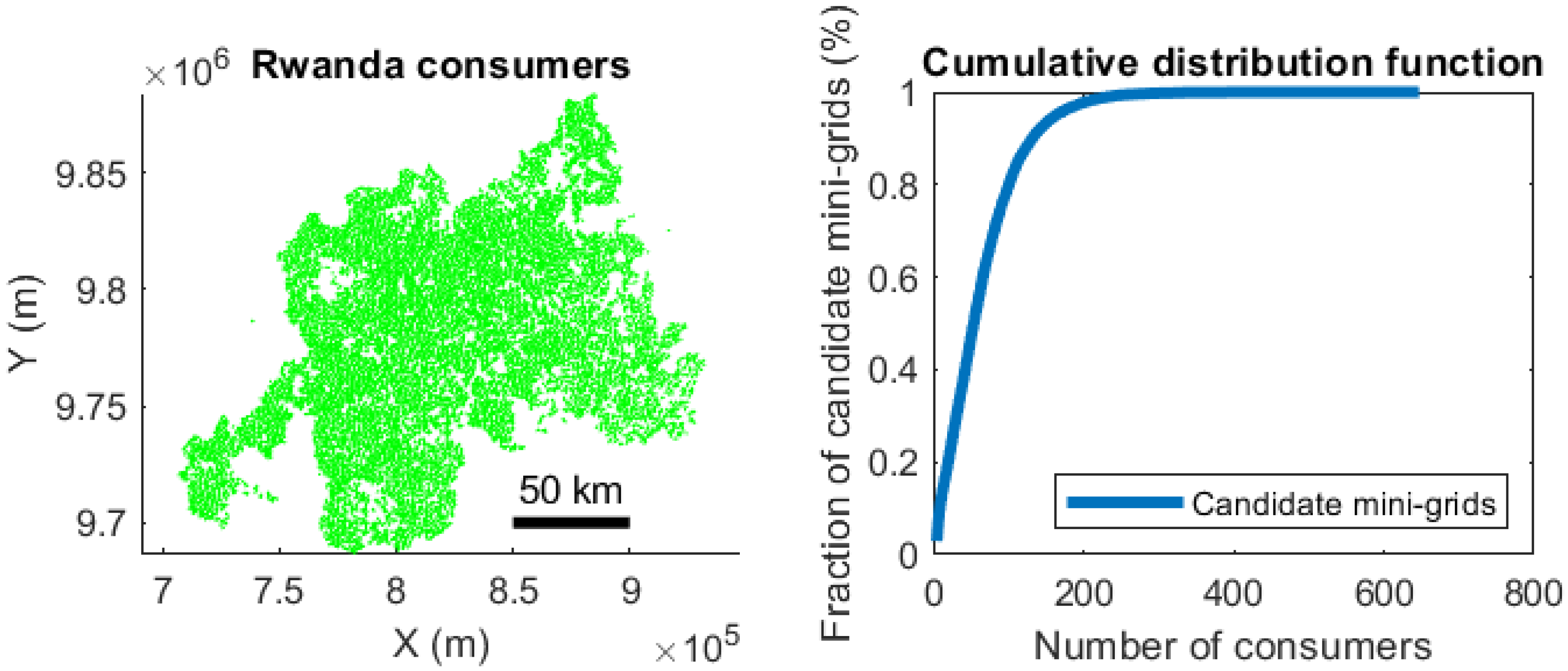
Rwanda has a total surface of 26,340 km² [57] (see Figure 5) and a population density of 525 people per km² of land area, being one of the countries with the highest population density in Sub-Saharan Africa [58]. The case study has 1,598,842 unelectrified consumers, and we use REM to group them into potential, realistic mini-grids. REM applies a clustering algorithm that groups the consumers into candidate mini-grids and grid extensions following a two-steps logic. In the first step (off-grid clustering), the model assumes that all consumers are electrified with off-grid alternatives and grid extensions are not considered. This first step is the one we use to group the consumers into potential mini-grids. Reference [15] provides a thorough description of REM’s clustering.

REM may only consider off-grid clusters of a specific size (i.e., with a minimum number of consumers or demand) when it determines the consumers to be electrified with mini-grids. In our analysis, we exclude off-grid clusters with less than five consumers as potential mini-grids. The off-grid clusters with less than five consumers account for 0.71% of the total number of consumers. The remaining off-grid clusters account for 24,381 candidate mini-grids.

The location of the consumers and the candidate mini-grid sizes are shown in Figure 5. Rwanda’s high density of consumers leads to considerably large candidate mini-grids, with an average size of 65.11 consumers. Many candidate mini-grids (97.73%) have at most 200 consumers, and the biggest candidate mini-grid has 647 consumers.

As a general trend shown in Figure 5, the number of candidate mini-grids of a certain number of consumers tends to decrease as the number of consumers increases (i.e., mini-grids with a large number of consumers are less frequent than mini-grids with a low number of consumers). For example, there are 713 candidate mini-grids with five consumers, whereas there are 128 candidate mini-grids with 100 consumers and only 14 candidate mini-grids with 200 consumers.

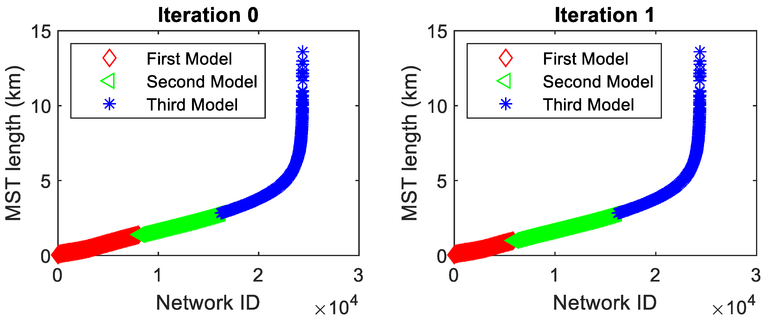
Our method groups the mini-grids into three linear models, and the shortest and the largest MST lengths are 34.93 m and 13.64 km, respectively. Figure 6 shows the mini-grids that our method assigns to the linear models.

In iteration 0 (see Figure 6), our method assigns the same number of mini-grids to the first, the second, and the third linear model. The quotients between the maximum MST length and the minimum MST length of the first, second, and third models are 39.99, 2.03, and 4.81, respectively. Therefore, the first model does not satisfy Equation (11). Since the maximum MST length of the first model is higher than 1 km, our method performs an additional iteration (iteration 1) to ensure that the first model satisfies Equation (11) or has a maximum MST length lower than 1 km.

After iteration 1, the first model has a maximum MST lower than 1 km (see

Table 3. Mini-grids assigned to each model.

Model	Condition for Assignation (m)	Number of Mini-Grids
First	$length\left(MST\right)<999.8$	5892
Second	$999.8\le length\left(MST\right)\le 2833.7$	10,362
Third	$2833.7<length\left(MST\right)$	8127

), and the remaining models satisfy Equation (11), so the network assignment procedure ends. Table 3 shows the number of mini-grids that are assigned to each model and the MST lengths that determine whether a mini-grid is assigned to a model.

For each model, the procedure selects a few representative mini-grids. The number of mini-grids is determined imposing that the marginal gain of having more mini-grids drops below 10%, and the candidate number of mini-grids considered are 25, 31, 40, 50, 63, 79, 100, 126, 159, and 200 (10 points logarithmically spaced between 25 and 200). We scale the MST length with a factor of 10,132.3 $/km and the aggregated demand with a factor of 0.4 $/kWh. 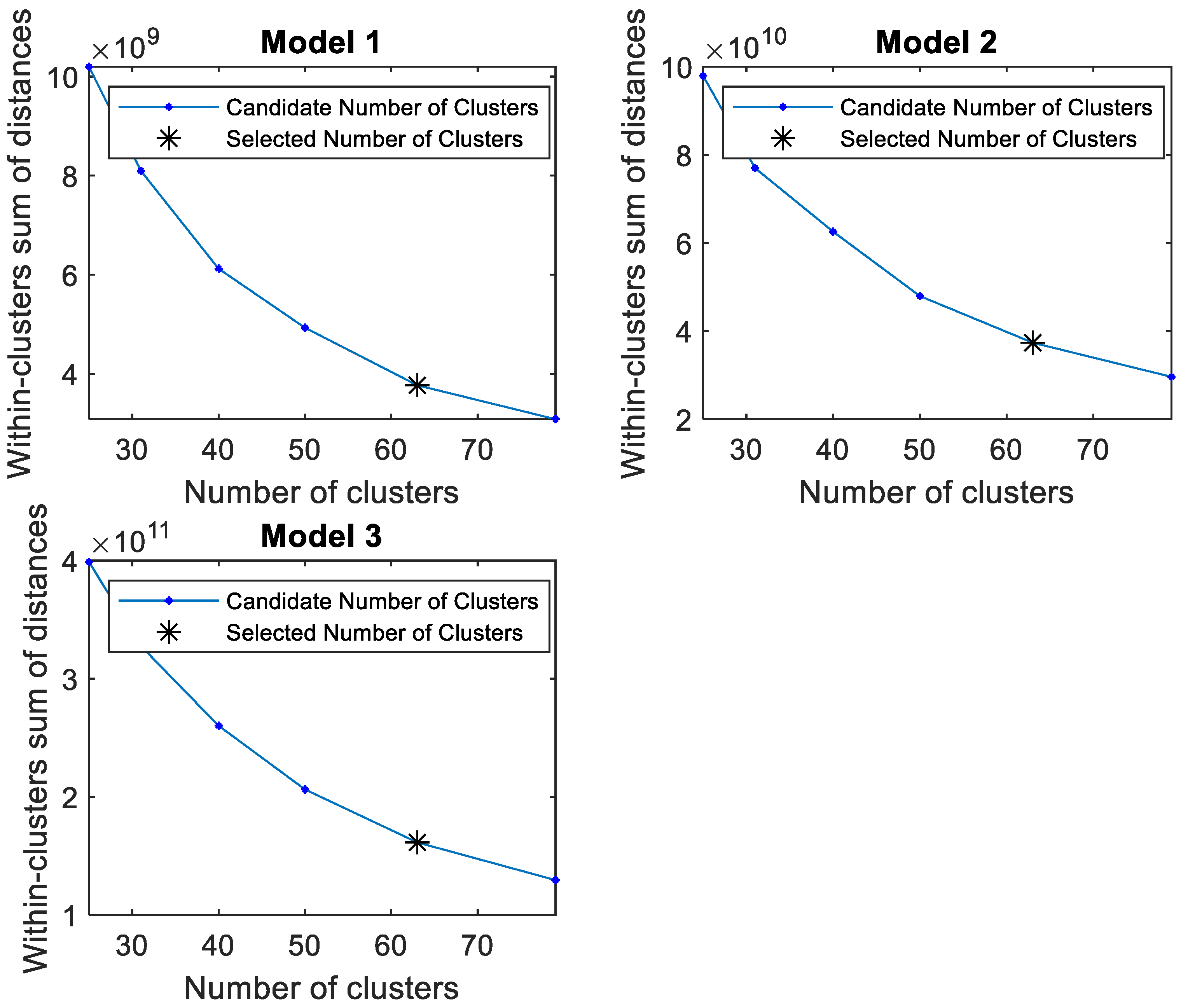Figure 7 shows the number of representative mini-grids (clusters) for each model.

The within-clusters sums of distances shown in Figure 7 for the second linear model are one order of magnitude higher than the within-clusters sums of distances of the first linear model. Similarly, the within-clusters sums of distances of the third linear model are one order of magnitude higher than the within-clusters sums of distances for the second linear model. This is very reasonable as the goal of the network assignment step is to assign mini-grids whose network costs have different magnitudes to different linear models.

The marginal gain of the within-clusters sum of distances related to having more mini-grids is more than 20% in the initial iteration (when the number of representative mini-grids goes from 25 to 31) for the three linear models shown in Figure 7. The marginal gain drops below 10% in the fifth iteration (when the number of representative mini-grids increases from 50 to 63) for all the linear models. The within-clusters sums of distances of the selected number of representative clusters (i.e., 63 for all the linear models) are less than half the within-clusters sum of distances of the initial number of representative mini-grids tested (25 mini-grids).

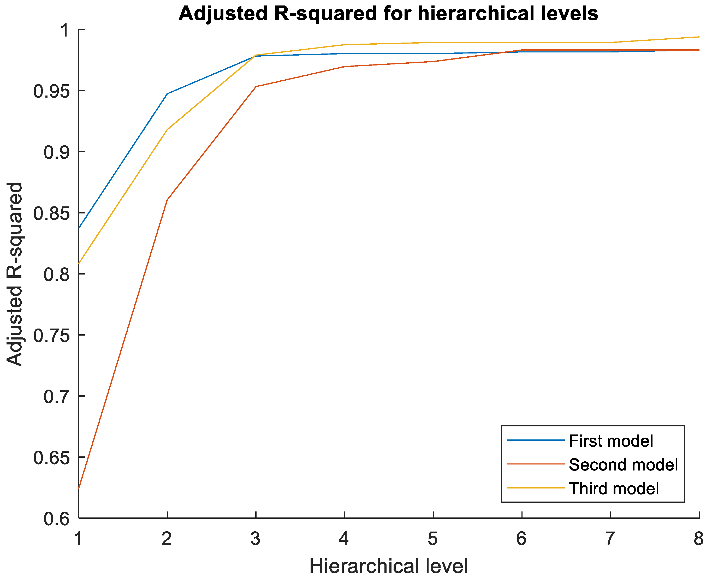
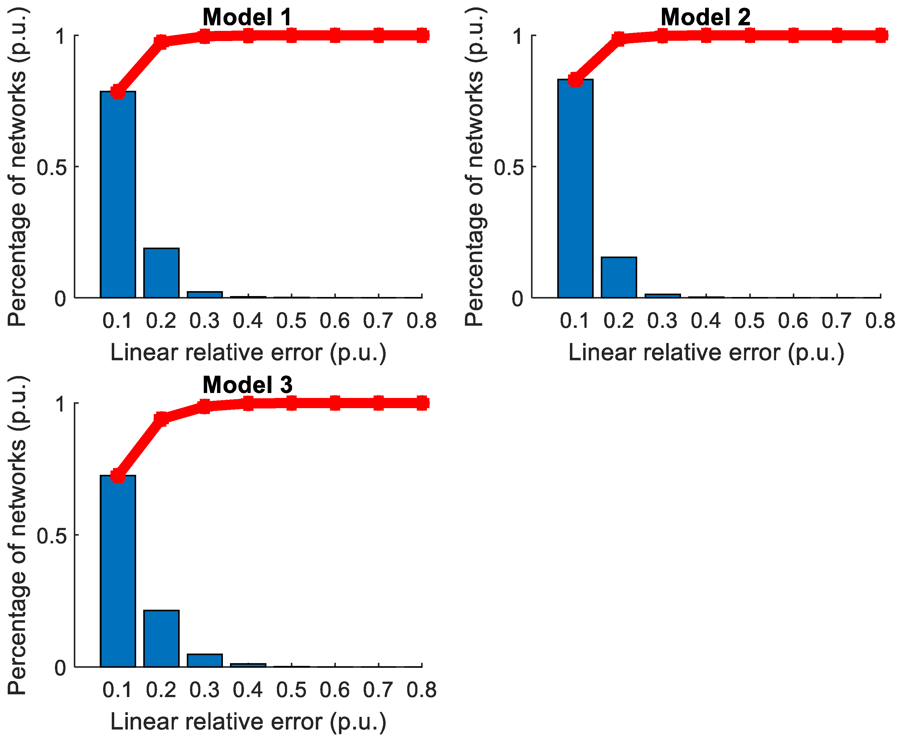
The method adjusts three linear models calculating the network costs of the representative mini-grids and using hierarchical regression. We consider that it is not worth adding more variables into the model when the marginal gain of the adjusted $R^2$ is less than 10%, which corresponds to the third hierarchical model in all cases (see Figure 8).

Although the three linear models have the same explanatory variables (length of the MST, number of consumers, and central moments of order two), it is still advantageous to have different linear models as the coefficients are different.

We compare the exact and approximated network cost of the 24,381 candidate mini-grids to obtain the relative linear error (defined as the absolute value of the quotient between the difference of costs and the real cost) that we incur with the model. Figure 9 provides the corresponding results.

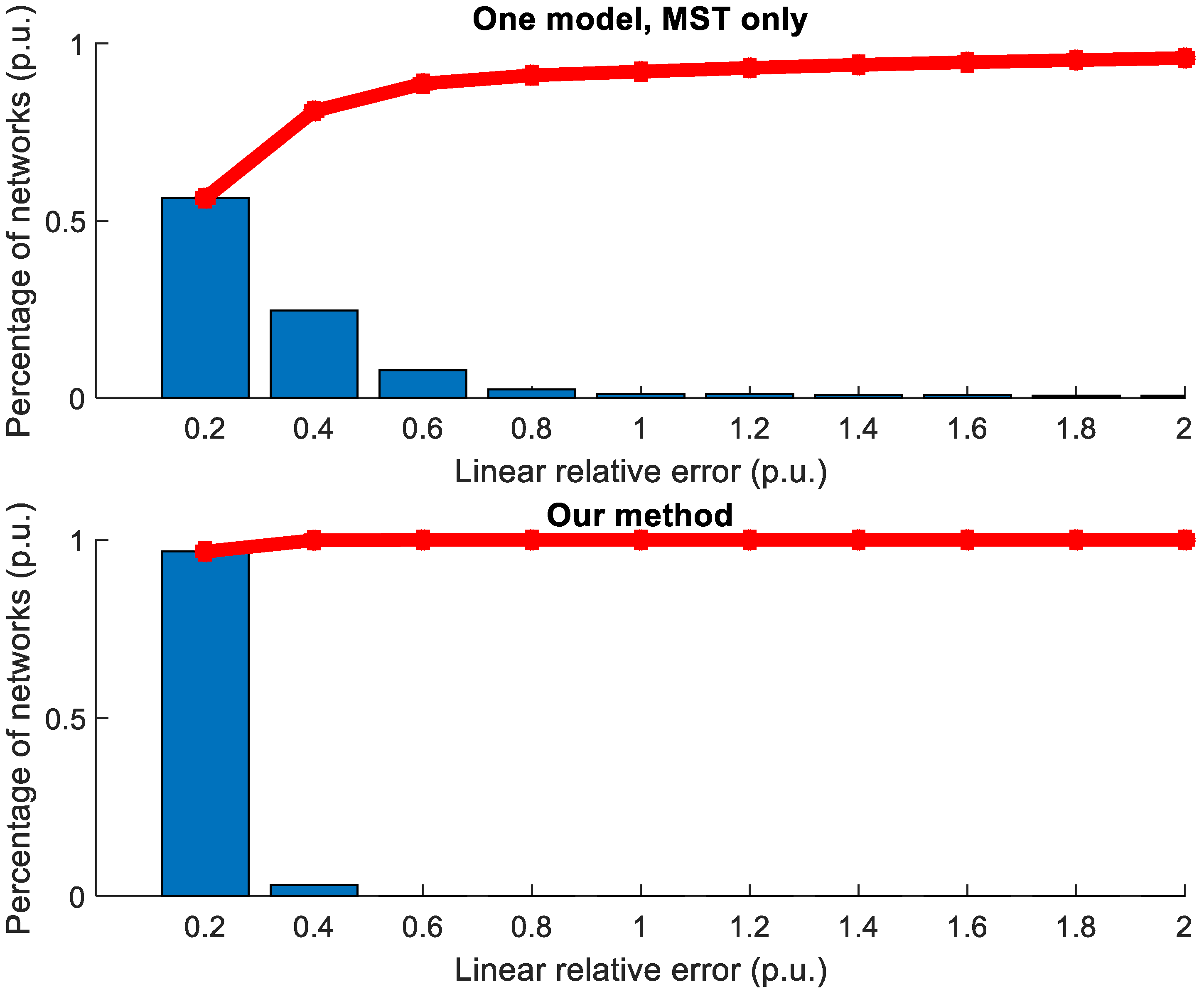
We also compare our method with a linear model that only considers the MST length (plus a constant term) to estimate the network cost. In this case, we directly force the model to use 200 representative networks instead of using the marginal gain procedure described in Section 3.2. Most regional planning tools apply techniques based on the calculation of an MST to calculate the network costs.

Figure 10 shows the linear error (p.u.) obtained for the 24,381 networks with both procedures. The naïve estimation provides a linear relative error lower than 20% for 56.36% of the networks, whereas our method obtains a linear relative error lower than 20% for 96.73% of the networks.

Figure 11 shows the linear absolute error obtained with both procedures (defined as the absolute value of the difference of costs). Our method obtains a linear absolute error lower than 100 $/yr for 83.57% of the networks, and the more straightforward procedure obtains the same error for only 57.73% of the networks. However, the difference between our method and the straightforward procedure is reduced as the annual cost threshold used for the comparison increases. For example, our method provides an absolute error lower than 300 $/yr for 99.21% of the mini-grids with our method, whereas the straightforward procedure obtains the same error for 91.28% mini-grids. Similarly, the absolute error is lower than 500 $/yr for 99.94% of the mini-grids with our method and 97.96% of the mini-grids with the straightforward method. We can conclude that the MST is a decent initial approximation of the network cost of mini-grids, but it should be noted that relatively low absolute errors may correspond to high relative errors and the straightforward procedure provides a linear relative error higher than 100% (i.e., an error well beyond a reasonable threshold) for approximately 7.92% of the mini-grids whereas our method always provides a linear relative error lower than 100% (see Figure 10).

Results show that our method significantly improves naïve approximations without increasing computation time considerably, as it requires only the calculation of accurate designs for less than 1% of the total mini-grids in this case study.

Table 4. Computation times needed to apply our method and calculate the network designs.

Our Method	Optimize Network of All Mini-Grids
21 min, 56.03 s	23 h, 52 min, 38.48 s

shows the computation times required to apply our method (which only optimizes the network designs of representative mini-grids) and to optimize network designs for all the mini-grids. The computation times were obtained with a Hewlett-Packard (HP), Palo Alto, CA, USA, computer with 16 GB of RAM and the Intel(R) Core (TM) i7-8550U CPU @ 1.80GHz 1.99GHz processor. The operating system of the computer is Windows 10 (64 bits).

The computation time needed to apply our method is 1.53% of the computation time required to calculate the network designs for all the mini-grids. The most time-consuming part of our method is the network optimization of the representative mini-grids, which lasts 16 min, 22.31 s.

5. Conclusions

Access to energy is a fundamental right of every individual, and substantial progress is necessary to achieve universal access to energy by 2030. Regional planning tools play a prominent role since a computer-based rural electrification plan based on rigorous analysis is undoubtedly more likely to be implemented, although other factors such as the regulatory or political background should not be neglected. A realistic electrification plan should provide a reasonable approximation of the necessary budget and cost estimations of the systems involved in the solution (i.e., grid extensions, mini-grids, and standalone systems). One such cost is the network cost of mini-grids.

Most computer tools estimate the network cost of mini-grids with quick rules of thumb based solely on spatial considerations, providing on-the-spot solutions at the expense of losing accuracy. However, it is possible to obtain accurate estimations of the network cost of mini-grids without explicitly obtaining the layout of each network design.

This paper presents a method that estimates the network cost of all the potential LV mini-grids of a large-scale electrification case. The algorithm uses a combination of spatial metrics (such as the MST length), electric metrics (such as demand and electric moments), and other metrics (such as the number of consumers) as potential drivers of the network cost of a mini-grid. The selection of adequate metrics is crucial as results heavily depend on them.

First, mini-grids are distributed among linear regression models based on their MST lengths to avoid assigning mini-grids with network costs of different orders of magnitude to the same linear model. Then, our method performs a k-medoids clustering for each linear regression model to obtain a reduced set of representative mini-grids. The k-medoids method considers the MST lengths and aggregated demands of mini-grids to determine the representative mini-grids.

Finally, our method calculates detailed network designs only for the representative mini-grids and uses the corresponding information to determine which metrics are key drivers of the network cost for each linear regression model. The calculation of such key drivers is done by applying hierarchical regression, which starts with a simple model and determines which metrics are worth incorporating into the model following a sequential process.

We compare the exact network costs of mini-grids with the estimations that our method provides in a realistic large-scale case study, where our method optimizes the network designs of less than 1% of the mini-grids to obtain the estimations. The computation time required to optimize the networks of all the mini-grids is approximately one day. In contrast, the computation time needed to apply our method is around twenty-two minutes.

We also compare our method with a more straightforward estimation that is aligned with the rules of thumb that some regional planning tools apply. Our method provides an estimation where the linear relative error is lower than 20% for 96.73% of the mini-grids, whereas the straightforward method provides an estimation where the linear relative error is lower than 20% for only 56.36% of the mini-grids. We also contrast the linear absolute errors, and our method obtains an error lower than 100 $/yr for 83.57% of the mini-grids, and the more straightforward procedure obtains the same error for 57.73% of the mini-grids. We can conclude that a straightforward method (such as the ones that regional planning tools apply) may lead to significant errors when estimating the network costs. Therefore, many regional planning tools could profit from the method presented in this paper, as their solutions would be based on accurate network costs that go beyond oversimplified calculations based on rules of thumb.

Regarding additional developments, the method should be expanded to estimate the cost of medium-voltage mini-grids too. Most of the steps of the current approach could hold for medium-voltage mini-grids, but it may be necessary to change the hierarchical order of explanatory variables and add new variables because transformers could account for a significant amount of the total network cost.

It would also be interesting to explore ideas that allow us to expand our method to incorporate the impact of topographical features of the terrain in the network cost estimation. Such topographical features include terrain slopes and penalized areas, and may substantially impact the network cost of mini-grids.

We could also study the impact of the parameter Q on the results that our method provides. The case study shows that our method performs well when Q is set to 10, but a sensitivity analysis would allow us to quantify the impact of Q and determine if other values of Q could lead to an improvement of our method.