Abstract
This paper proposes a method to detect disconnection faults and their exact location in PV systems. The proposed method injects multiple frequencies into a PV system with a transmitter and detects the injected signal using a receiver. The signal detected by the receiver exhibits different frequency characteristics on a disconnection failure. Based on this characteristic, a disconnection failure can be detected. In addition, by detecting the frequency radiated through the disconnection point, the exact disconnection point can be detected.
1. Introduction
The international community has agreed to submit to the Long-Term Low Greenhouse Gas Emission Development Strategies (LEDS) to the United Nations (UN) by 2050 in accordance with the Paris Agreement. Accordingly, countries globally have established plans to achieve net zero carbon dioxide emissions to control climate change. The International Energy Agency (IEA), in a special report, proposed to achieve net zero emissions by 2050; however, it did not consider how energy is produced, transported, and used globally. The report predicted that by 2050, the global energy demand will decline by approximately 8% compared to today; however, the economy will be double in size and the population will grow by 2 billion people. More than 90% of electricity generation comes from renewable energy sources, and when wind and solar power are combined, it will account for nearly 70%; therefore, the PV system is predicted to be the most important energy source in the future [1].
In a PV system, the characteristics of the PV module (or solar cell), system design, and installation method (slope, direction, string configuration, etc.) have a decisive effect on its energy production. In addition, environmental factors, such as shade, pollution, soiling, and snow, also have the same effect on PV systems [2].
Electrical disconnection of PV arrays is a common problem in all PV systems [3]. It may occur due to the fact of electrical connection failure and related problems owing to cable or connector damage, connector corrosion, or poor mechanical connection. A ground fault occurs when a PV system is disconnected causing power loss of an individual PV array or the entire system [4]. A PV system is composed of several PV modules connected in parallel or in a series, and the performance degradation and failure or connection problem of the modules constituting the PV system cause overall power loss [5,6,7,8,9]. Therefore, detecting and finding these defects due to the electrical differences is an important factor in the reliability of PV systems [10].
Various methods are used to detect string errors and disconnections in PV systems. Current and voltage monitoring can warn of string problems, but it is difficult to detect the disconnection [11]. Infrared imaging techniques, such as electroluminescence [12,13], visual inspection, and unmanned aerial vehicles [14], are useful for identifying damage to the module itself but are unable to confirm problems in cable connections behind the module [15]. In addition, time–domain reflectometry (TDR) and spread-spectrum time–domain reflectometry (SSTDR) methods for finding problems, such as disconnection, using frequency have been proposed. These methods can detect disconnection and changes in electrical characteristics; however, to determine the exact location of disconnection, it is necessary to know in advance the frequency variation characteristics of the measuring device and the characteristics of the PV system such as impedance, length of string, and number of modules [16,17,18].
In the electrical equivalent circuit of a solar cell under AC, the solar cell has an internal parallel capacitor. The capacitor is an open circuit for DC, but it has a reactance value that varies with the frequency in the AC [19,20,21,22,23,24,25,26,27,28,29]. This paper proposes a method for detecting the disconnection failure and failure position of a PV system using these characteristics of the solar cell. In this study, multiple frequencies were simultaneously injected into both terminals (i.e., positive and negative poles) of a PV system, and disconnection failure were detected according to the characteristics of the injected frequencies. When a disconnection fault occurs in the PV system, the disconnected part radiates a signal, similar to a radio transmitter [30]. This signal is detected by the receiver, and the disconnection fault is determined by the size and pattern of the detected signal. Via the method proposed in this paper, the characteristics of a transmitter and receiver using the PSIM were simulated, the transmitter and receiver designed and created, and its validity proved through experimental results.
This paper presents the configuration of the electrical characteristics and failures of PV systems in Section 2; PV system disconnection, fault detection, and fault point detection using multiple frequencies in Section 3; the simulation and experimental results in Section 4, and the conclusion in Section 5.
2. Electrical Characteristics and Failure of a PV System
2.1. Electrical Characteristics of a PV System
A PV array is generally composed by connecting several PV strings, and each PV string connects several PV modules in a series. When PV modules are connected, the overall I–V characteristics are determined by the interactions among the PV modules, and the module or string with the lowest performance has the greatest influence on the overall characteristics [5,31,32].
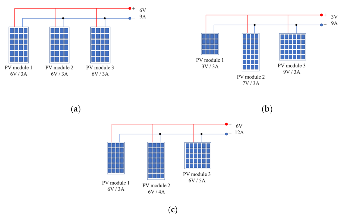
Figure 1 and Figure 2 show the electrical characteristics of the series and parallel connections of the PV modules. Figure 1a shows a case when all modules with the same electrical characteristics are connected, and Figure 1b,c show the case in which the characteristics of voltage and current are different. In a series circuit, each voltage is added, but the current flowing inside must be the same. In Figure 1b, although the value of the voltage is different, the current flow is the same, so the output of the entire module is equal to the sum of the outputs of each module. However, Figure 1c shows that the value of the voltage is the same, but the current flow is different. In this case, the current flowing is the current of the PV module with the lowest current depending on the characteristics of the DC circuit. Thus, only 19 W, which is 27% of the total capacity of 69 W, will be available. In particular, the capacity of Module 3 in Figure 1c is 45 W (9 V, 5 A), but only 9 W (9 V, 1 A), which is only 20%, is used.
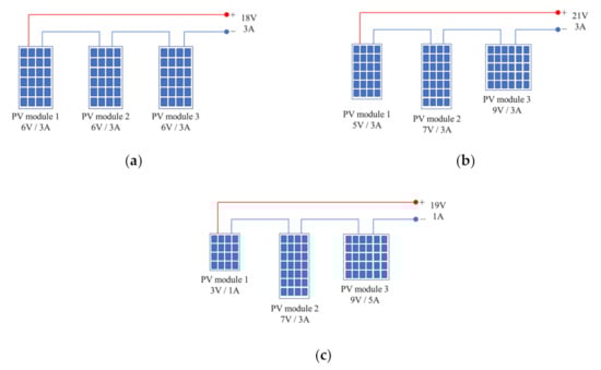
Figure 1.
Electrical characteristics for a series connection of PV modules: (a) PV modules in a series with the same characteristics; (b) PV modules in a series with different characteristics (i.e., voltage); (c) PV modules in a series with different characteristics (i.e., current).
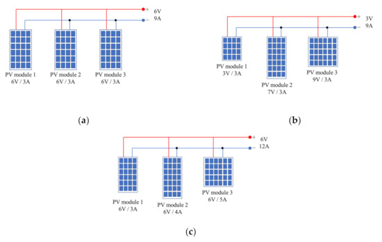
Figure 2.
Electrical characteristics for parallel connection of PV modules: (a) PV modules in parallel with the same characteristics; (b) PV modules in parallel with different characteristics (i.e., voltage); (c) PV modules in parallel with different characteristics (i.e., current).
Figure 2 shows the electrical characteristics of the parallel connections of the PV modules. Figure 2a shows a case where the characteristics of all PV modules are the same, and Figure 2b,c show a case in which the voltage and current are different, respectively. In a parallel circuit, currents are summed despite being different; however, the voltages must be the same. When the voltages are different, the voltage of the parallel circuit becomes the voltage of the lowest PV module. Therefore, the total output for Figure 2c with the same current and different currents is the sum of the outputs of each module; however, for the case of Figure 2b with different voltages, the total voltage becomes the voltage of Module 1, which is the lowest voltage, and the total output becomes 27 W (3V × (3A + 3A + 3A)), which is 47% of the available 57 W (9 W + 21 W + 27 W). In particular, the output capacity of Module 3, which has the highest voltage, has the lowest efficiency because it is lowered to 9 W, which is 33% of the maximum output of 27 W.
A PV system is configured by connecting PV modules and arrays in a series and parallel for a required output; however, an electrical difference among PV modules may cause unexpected power loss. Electrical differences among PV modules and arrays may occur because of the characteristics, shadows, and failures of the PV modules. Therefore, it is important to reduce the differences in electrical characteristics.
2.2. Failure of PV Systems
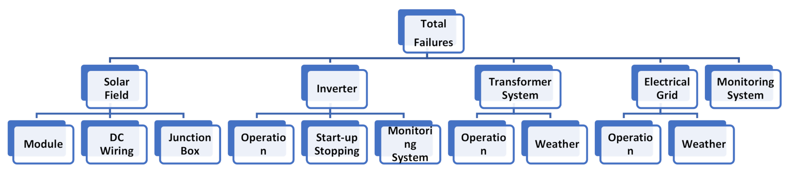
The failure classification according to the equipment constituting the PV system can be expressed as follows (Figure 3).
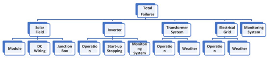
Figure 3.
Classification of failures according to the equipment in PV systems.
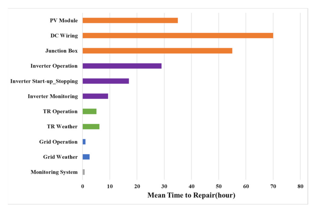
Figure 4 shows the mean time required to repair each failure. The repair time of the solar field in Figure 3 was longer than that of another failure. Therefore, a fast and simple method to detect disconnection faults is required [33].

Figure 4.
Mean time to repair failures in PV systems.
3. Proposed Method (Multiple Frequency Injection Method)
3.1. AC and DC Characteristics of Solar Cells
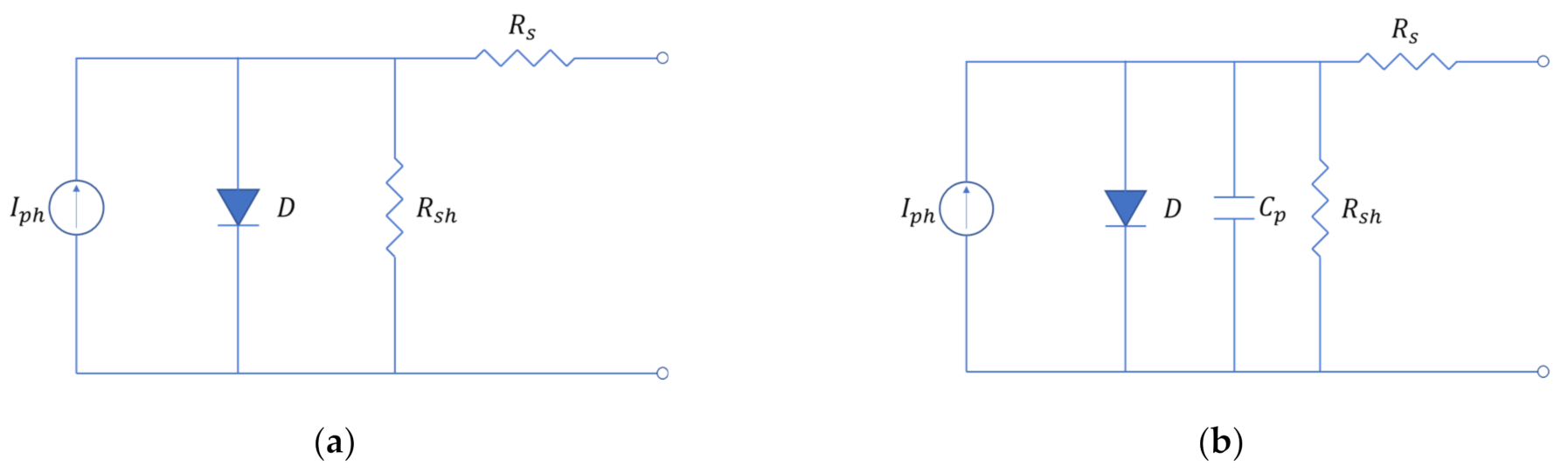
Figure 5 shows the equivalent circuit of a solar cell for DC and AC. Figure 5a,b are an equivalent circuit for DC and AC, respectively. In DC circuits, capacitors are in an open state, so they are omitted from DC circuits, but in AC circuits, the reactance component of the capacitor changes according to frequency, so it is included in the equivalent circuit to show the effect [34,35,36,37,38,39,40,41,42,43,44].
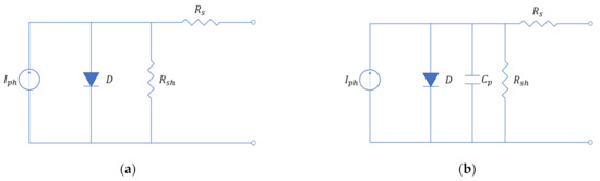
Figure 5.
Equivalent circuit of a solar cell: (a) DC equivalent circuit; (b) AC equivalent circuit. .
In the equivalent circuit of an ideal solar cell, the parallel resistance is infinite, and the series resistance is zero. Various methods have been proposed to calculate in the AC equivalent circuit of a solar cell, and the capacitor changes according to the cell’s voltage, level of irradiance, frequency, and temperature [19,20,21,22,23,24,25,26,27,28,29]. During the change from the reverse bias to the forward bias voltage of the cell, there is an inflection point where the capacitor increases gradually and then rapidly increases [19,20,21,22]. As the levels of irradiation [26,27] and temperature [19,27,28,29] increase, the capacitor increases proportionally.
3.2. Disconnection Detecting Method Using Multiple Frequency Injection
This paper proposes a method to detect the disconnection failure and failure location of a PV system using the capacitor characteristics of the AC equivalent circuit of a solar cell. Because a solar cell outputs DC according to the intensity of solar radiation, it is difficult to distinguish a normal signal from a faulty signal when a DC signal is used as a reference. Therefore, this paper proposes a method to detect faults and determine the exact location of faults in PV systems. The method proposed in this paper injects high frequencies into both terminals (i.e., positive and negative poles) of a PV system and analyzes the characteristics of the injected frequencies.
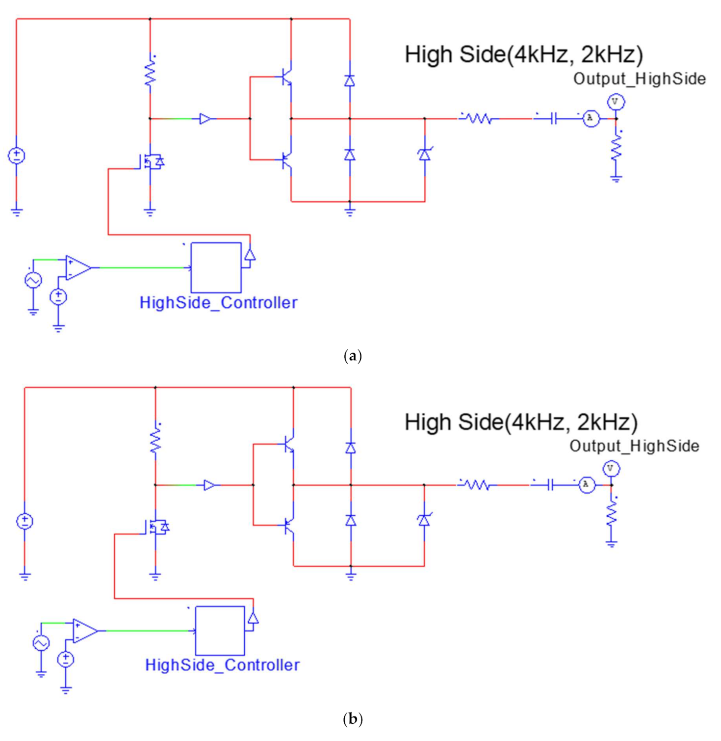
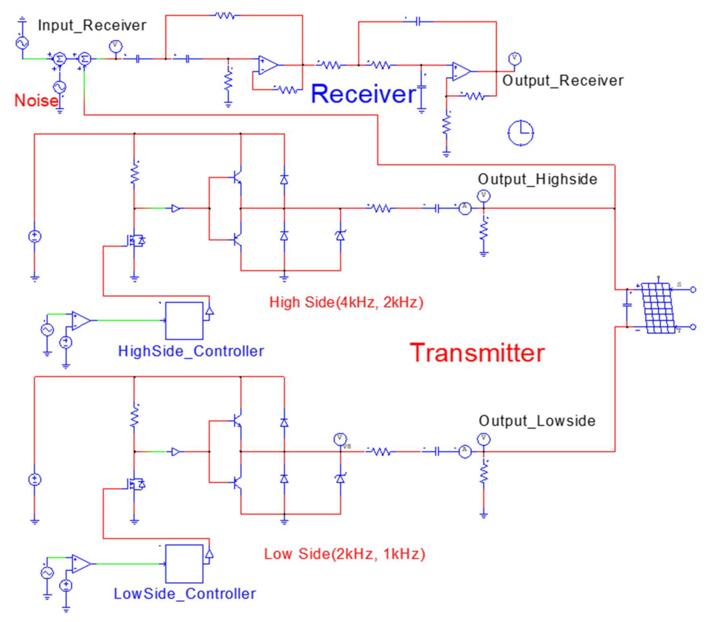
Figure 6 shows a transmitter that generates a frequency signal to detect the disconnection of a PV system. Figure 6a shows a high side circuit that sequentially generates relatively high frequencies of 4 and 2 kHz, and Figure 6b shows a low side circuit that sequentially generates relatively low frequencies of 2 and 1 kHz. The HighSide_Controller and the LowSide_Controller in Figure 6a,b control the switching frequency for the high side and low side, respectively.

Figure 6.
The frequency generating circuit: (a) high side circuit in the transmitter; (b) low side circuit in the transmitter.
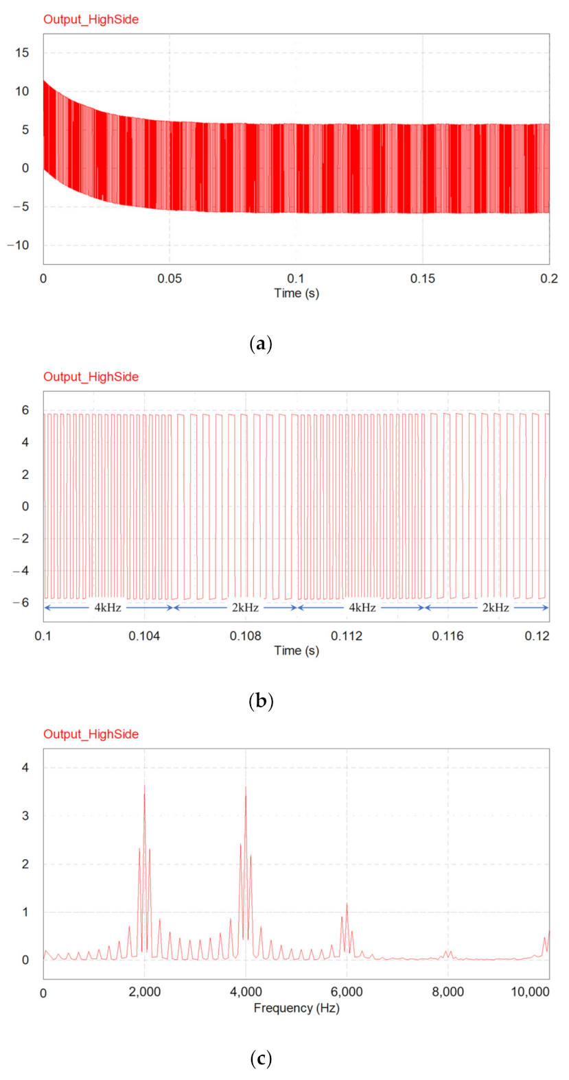
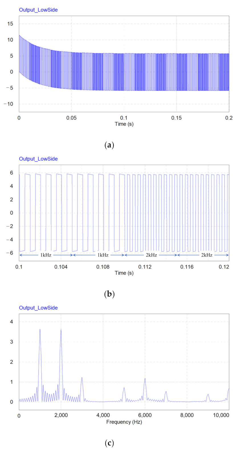
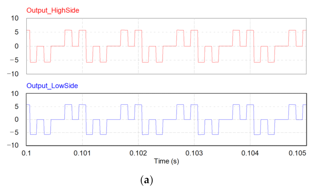
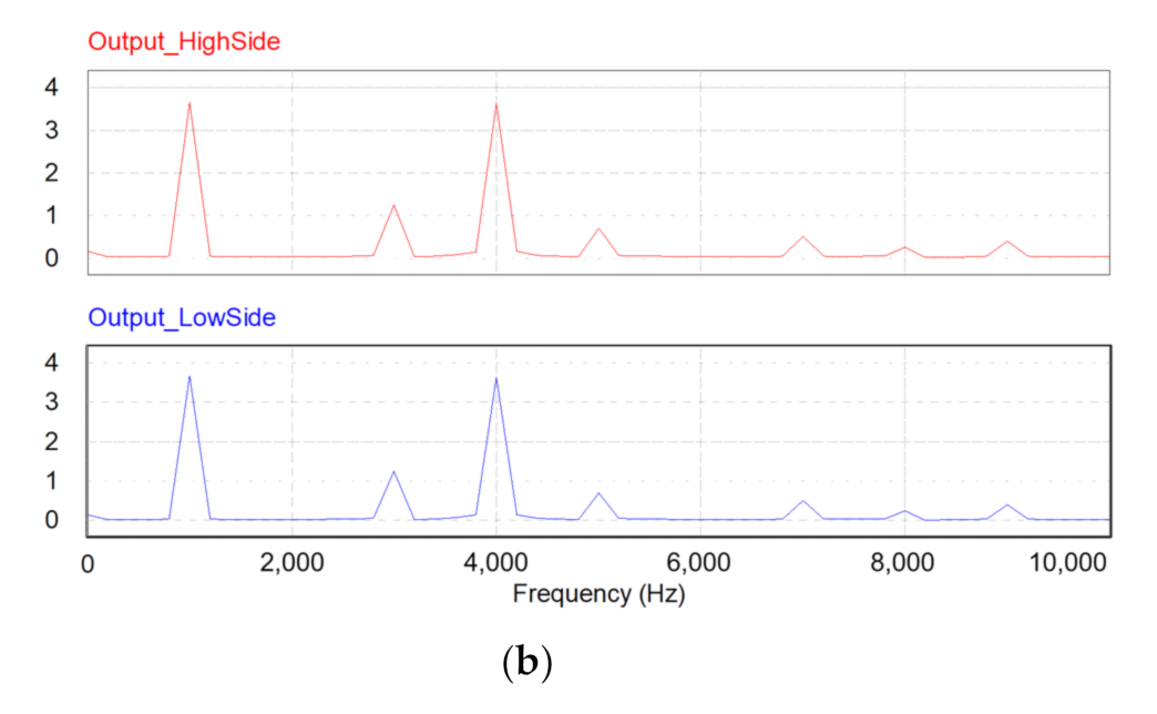
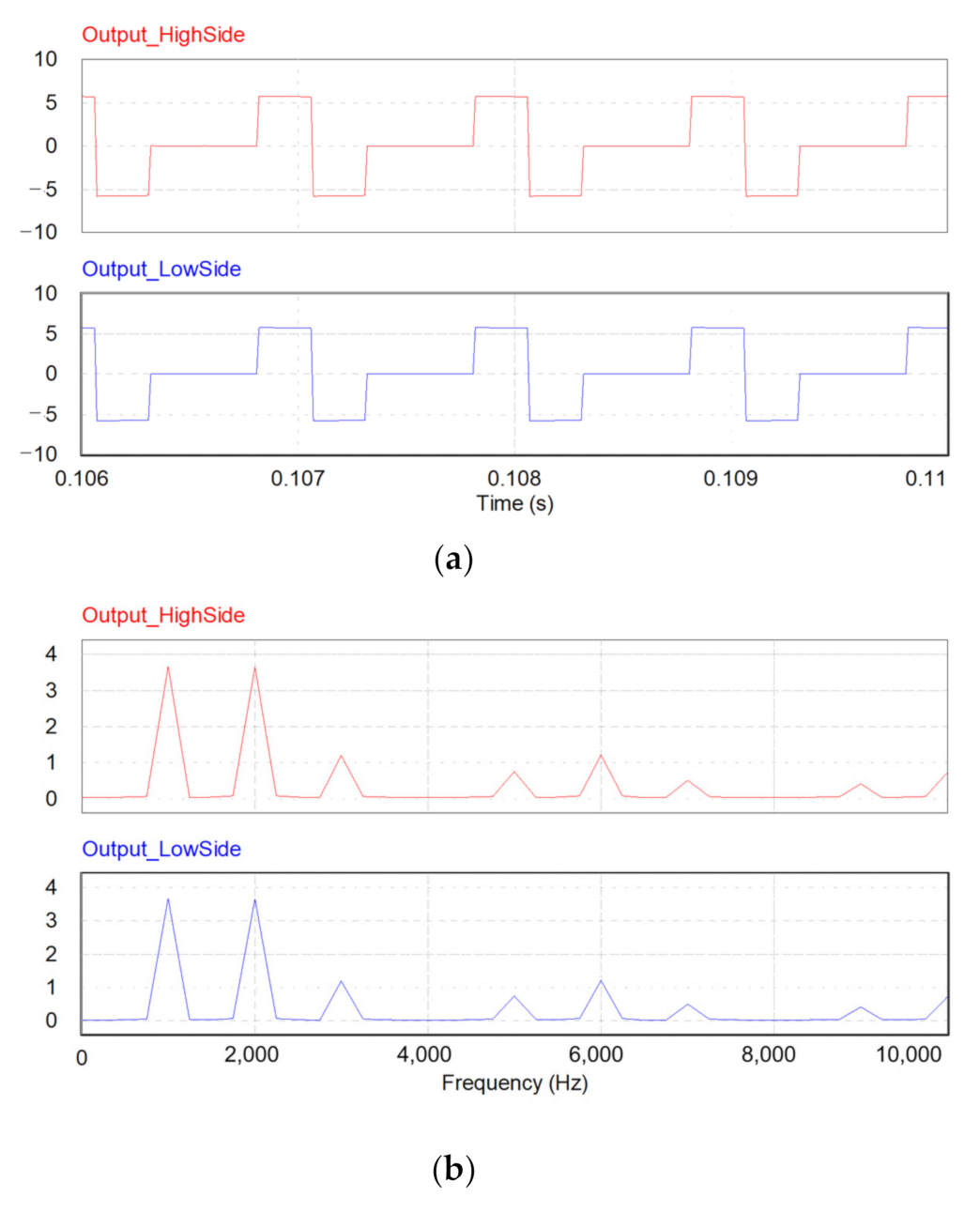
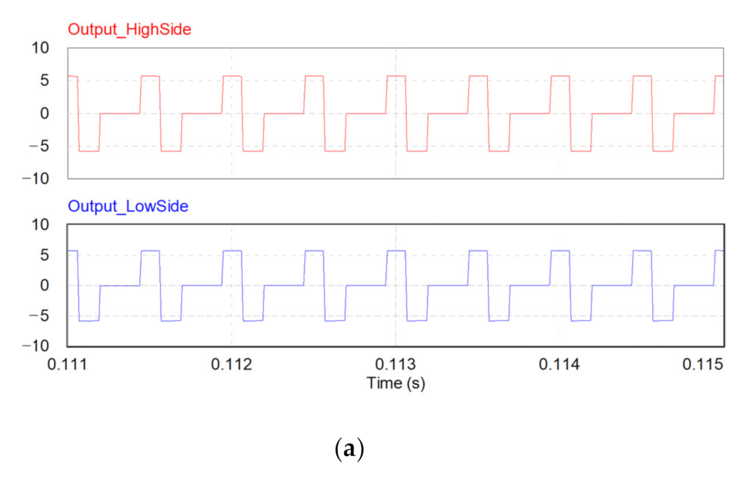
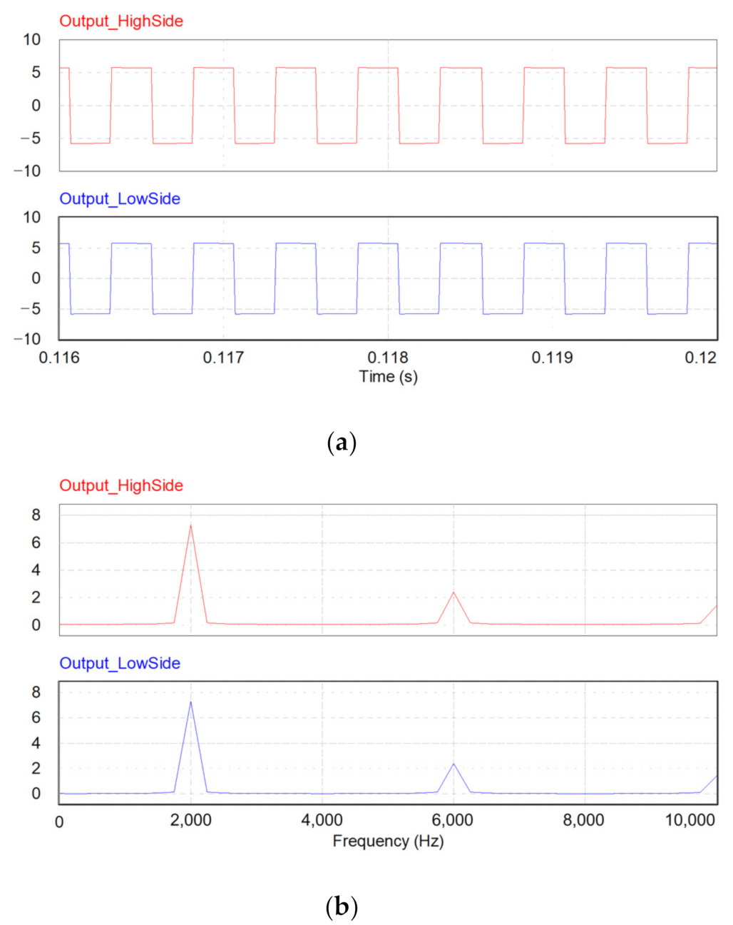
Figure 7 and Figure 8 show the output characteristics of the high side and low side in Figure 6, respectively, and Table 1 shows the frequency change generated by the frequency-generating circuit. When the frequency change period is 5 ms, the high side repeats the two frequencies in the order of 4 kHz→2 kHz→4 kHz→2 kHz, and the changing sequence of the low side frequencies is 1 kHz→1 kHz→2 kHz→2 kHz. According to the change order of the high side and low side frequencies, four different waveforms are created when the frequencies of both sides overlap. Therefore, when the frequency generated by the transmitter is injected into both terminals of the PV system under a normal state (no disconnection failure occurs), changes in the four frequencies can be detected.

Figure 7.
Frequency characteristics of the High Side of the transmitter: (a) High Side output; (b) High Side frequency; (c) High Side FFT.
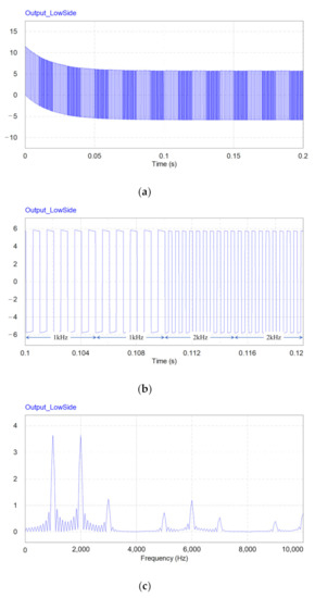
Figure 8.
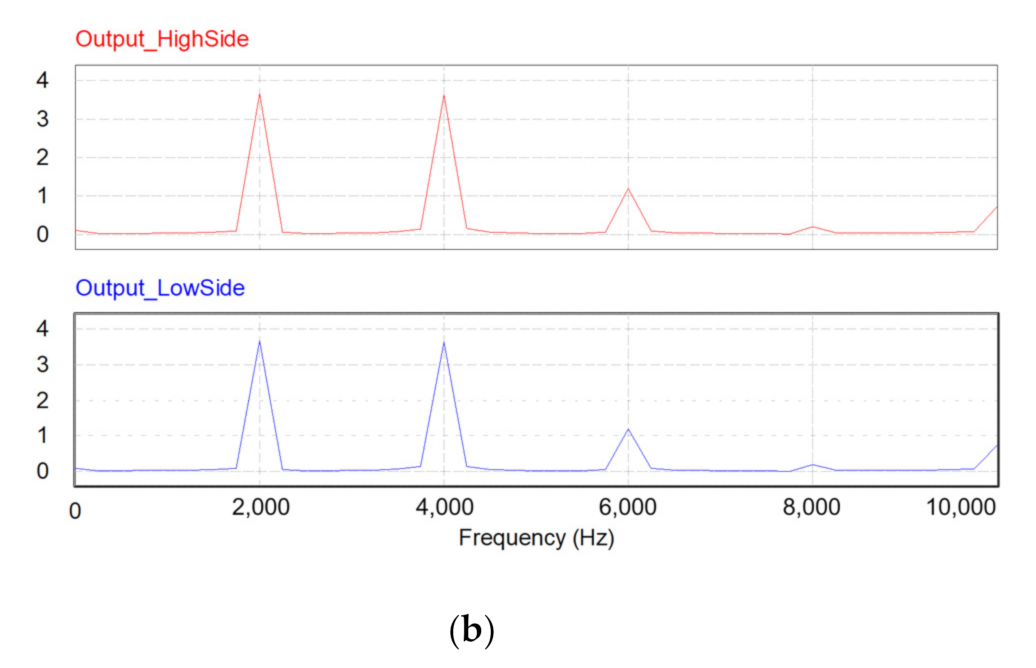
Frequency characteristics of the low side of the transmitter: (a) low side output; (b) Low side frequency; (c) low side FFT.

Table 1.
Comparison of frequency variation characteristics.
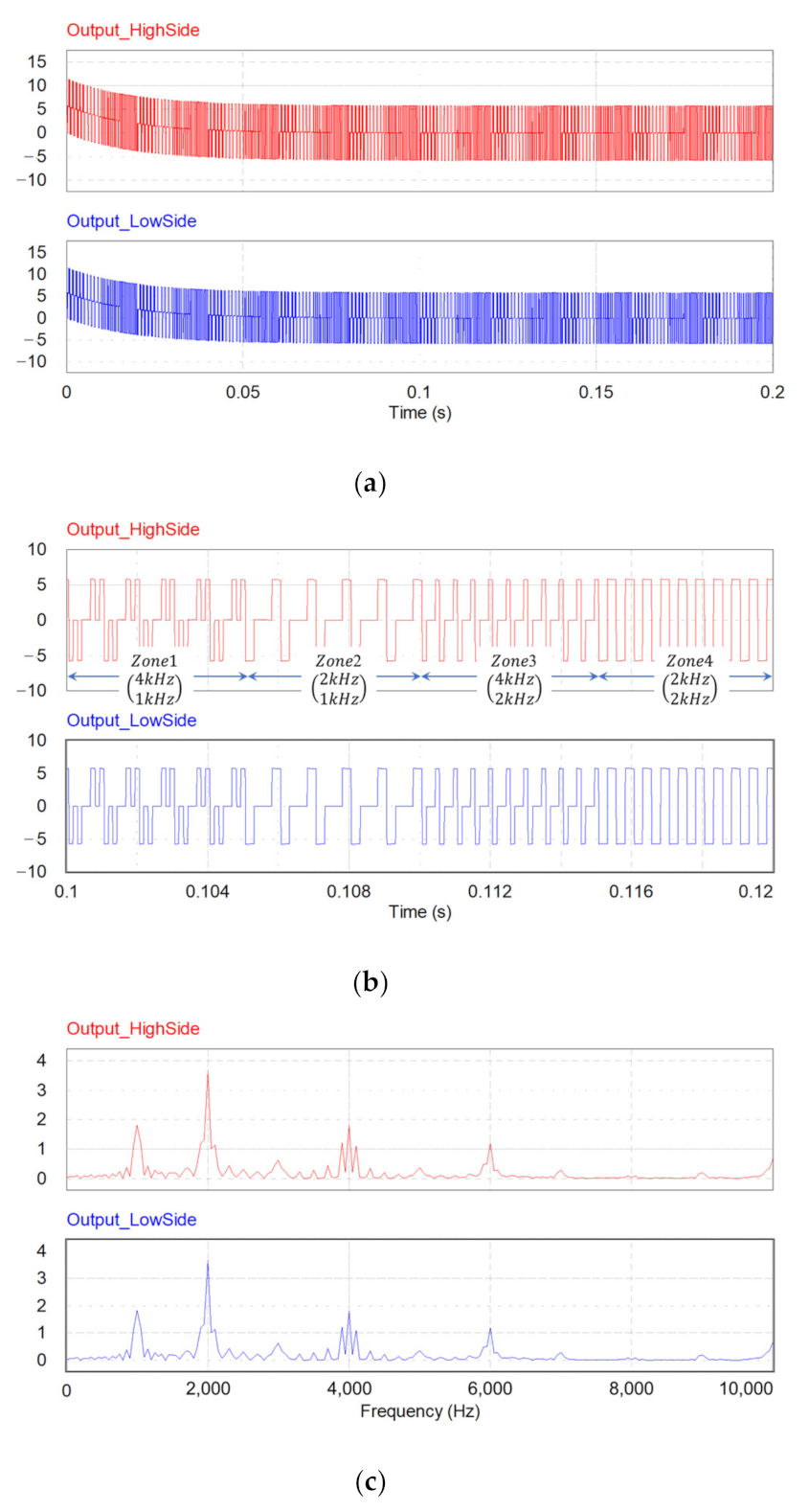
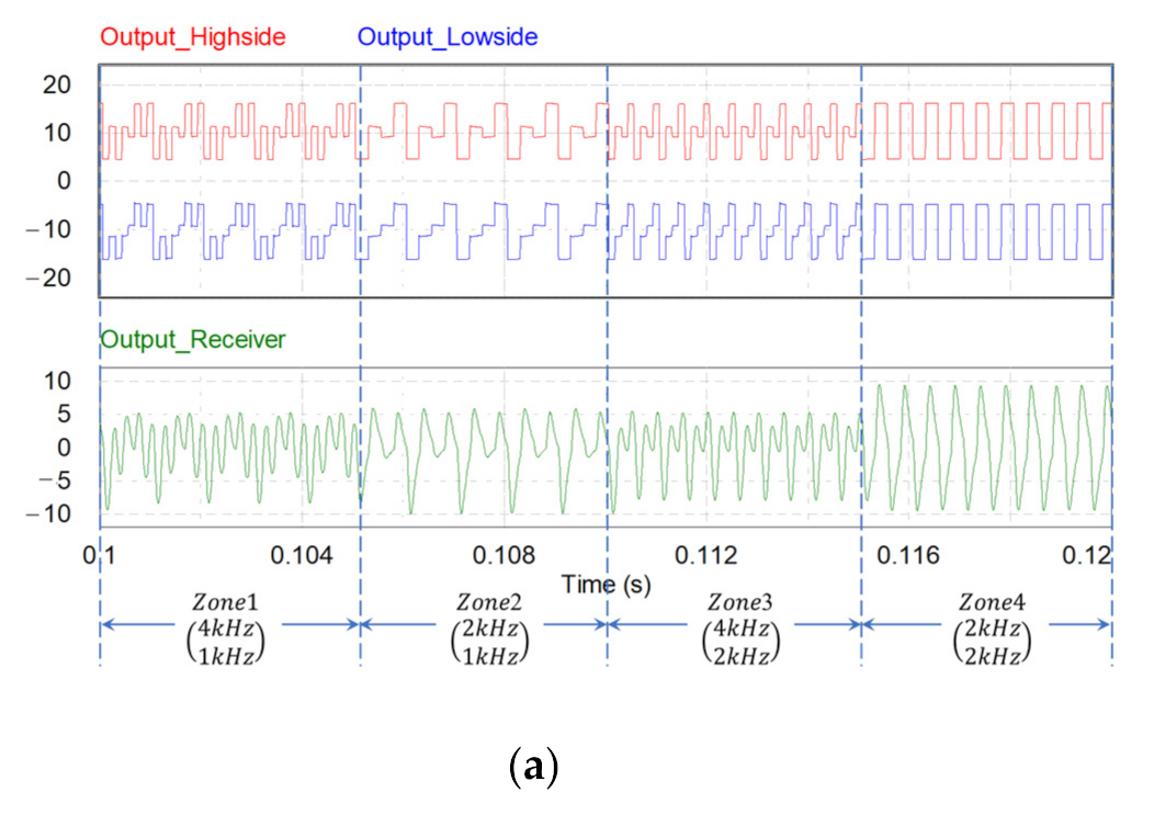
Figure 9, Figure 10, Figure 11, Figure 12, Figure 13 show the characteristics of the overlapped frequencies under a normal state. Figure 10 shows Zone 1 of Figure 9, Figure 11 shows Zone 2 of Figure 9, Figure 12 shows Zone 3 of Figure 9, and Figure 13 shows the frequency and FFT characteristics of Zone 4 of Figure 9, respectively. As the signals overlap without disconnection failure, the signals on the high side and low side are the same. In the FFT characteristic, the magnitude of the injected frequency in each zone was high, as shown in Table 1.
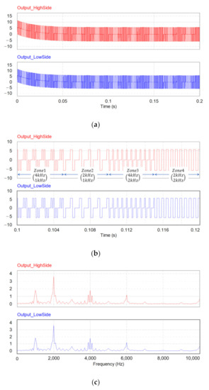
Figure 9.
The high side and low side frequency overlap under normal state: (a) frequency variation characteristics; (b) expansion of the frequency variation characteristics; (c) FFT characteristics.
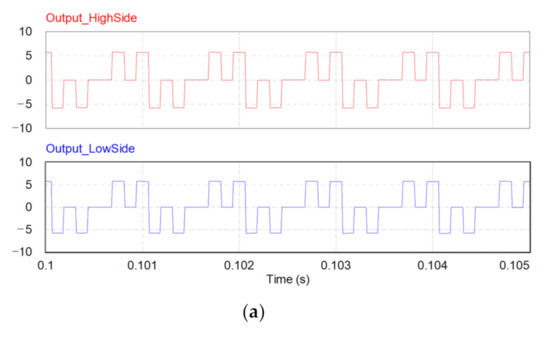
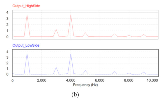
Figure 10.
Frequency and FFT characteristics of Zone 1: (a) frequency characteristics of Zone 1 (4 kHz + 1 kHz); (b) FFT characteristics of Zone 1 (4 kHz + 1 kHz).
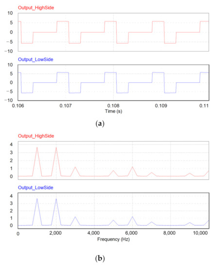
Figure 11.
Frequency and FFT characteristics of Zone 2: (a) frequency characteristics of Zone 2 (2 kHz + 1 kHz); (b) FFT characteristics of Zone 2 (2 kHz + 1 kHz).
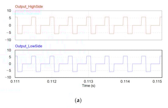
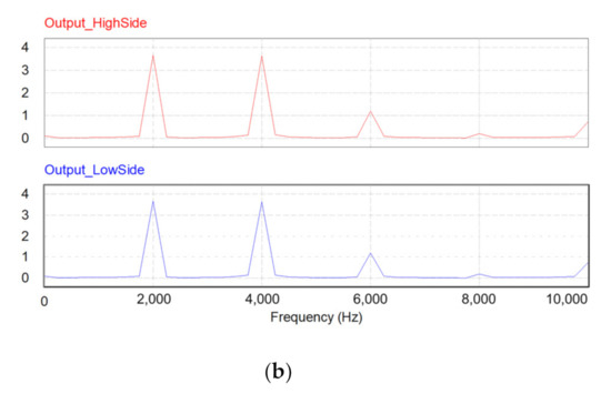
Figure 12.
Frequency and FFT characteristics of Zone 3: (a) frequency characteristics of Zone 3 (4 kHz + 2 kHz); (b) FFT characteristics of Zone 3 (4 kHz + 2 kHz).
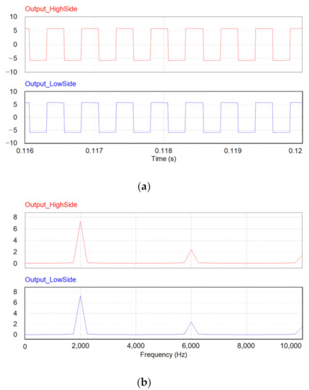
Figure 13.
Frequency and FFT characteristics of Zone 4: (a) frequency characteristics of Zone 4 (2 kHz + 2 kHz); (b) FFT characteristics of Zone 4 (2 kHz + 2 kHz).
3.3. Detection Method of the Disconnection Position in the PV System
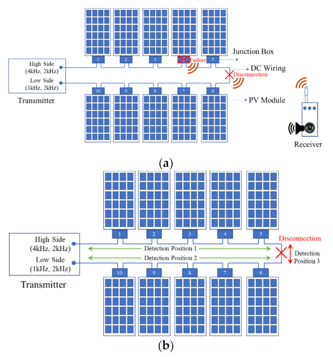
Figure 14 shows the method for disconnection failure position detection. When disconnection failure occurs in the junction box or DC wiring, the frequencies injected from the transmitter do not overlap and each has a connected frequency value. When disconnection occurs, the disconnection point operates like an antenna that radiates a frequency to the outside, and this signal is converted into sound through a receiver so that the exact disconnection fault location can be detected. In Figure 14b, the detection area is divided into three areas based on the disconnection failure point. Detection Area 1 and detection area 2 are the sections where the high side and low side are connected, respectively. In these sections, only each input signal is detected by the receiver. In detection area 3, in which the disconnection occurs, the transmitter’s input signal from both terminals of the PV system is radiated to the outside through the disconnected part; thus, both signals are detected by the receiver. Therefore, it is possible to detect the location at which the disconnection fault occurred.

Figure 14.
Detection method the disconnection positions in a PV system: (a) disconnection detecting method; (b) classification of the detecting area.
4. Results of the Simulation and Experiments
4.1. Results of the Simulation
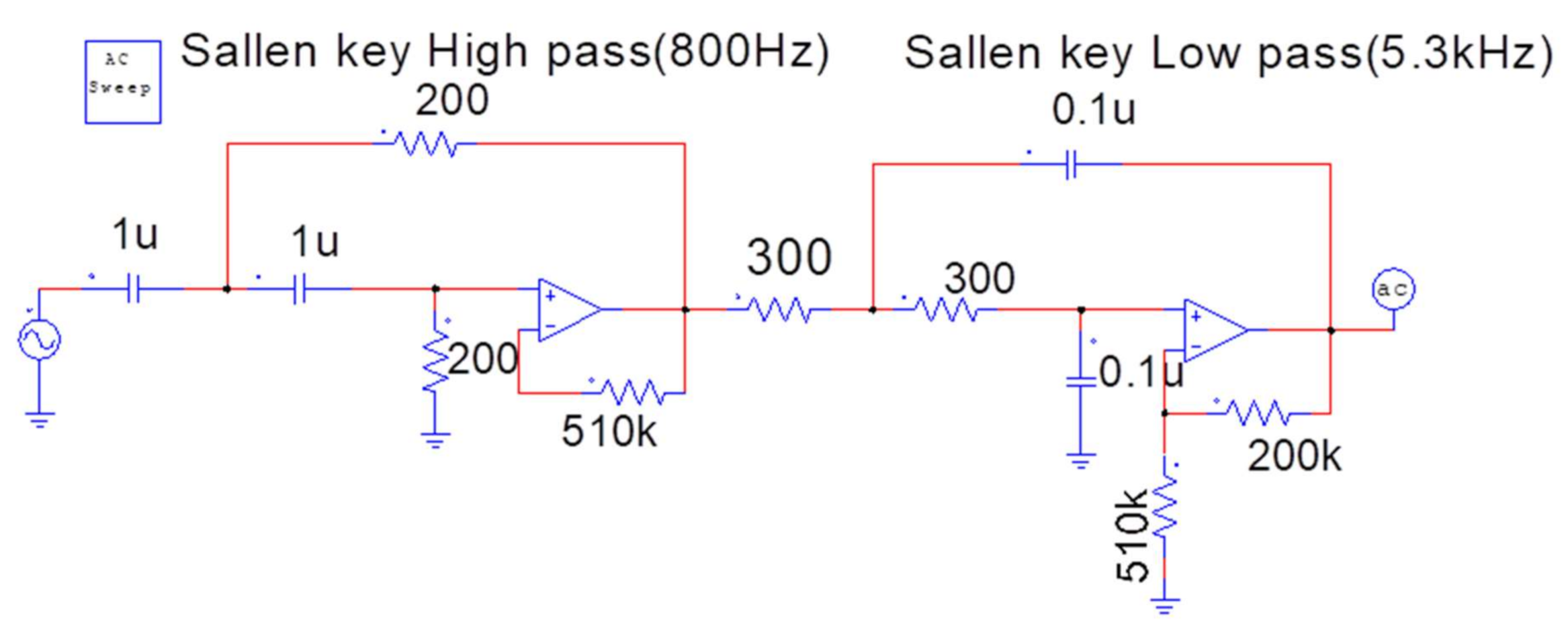
Figure 15 shows the receiver filter circuit used to detect the frequency generated by the transmitter. To detect only the signal generated by the transmitter, except for the frequencies used around the PV system, the receiver was designed as a band-pass filter. The band-pass frequency of the filter circuit was set from 800 Hz to 5.3 kHz. The range of this value was lower than the transmitter’s lowest frequency of 1 kHz and higher than the highest frequency of 4 kHz.
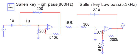
Figure 15.
Active filter circuit for the receiver.
Figure 16 shows the circuit used to analyze the characteristics of the transmitter and receiver. To analyze the characteristics of the transmitter and receiver, the PV module was connected to both terminals of the transmitter’s high and low sides, and the signal was input into the receiver and the characteristics were analyzed. In addition, a noise input part was added to analyze the characteristics of the receiver’s disturbance.

Figure 16.
Transmitter and receiver circuit for disconnection failure detection.
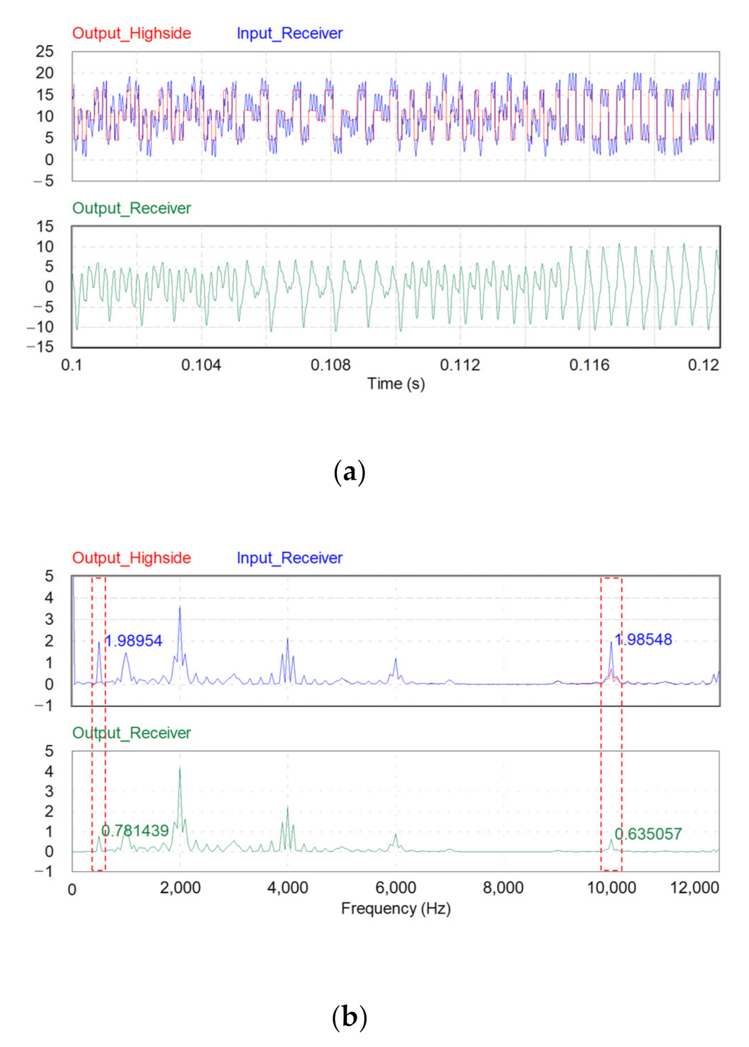
Figure 17 shows the response characteristics of the transmitter and receiver in the normal state when there is no disconnection in the PV system. The signals from the high side and the low side of the transmitter overlap in the normal state, and the receiver detects this signal from the transmitter. Therefore, the frequency components of the transmitter and receiver are almost similar in the FFT characteristics of Figure 17b.
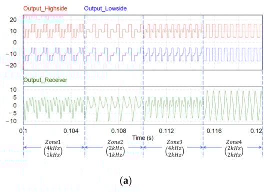
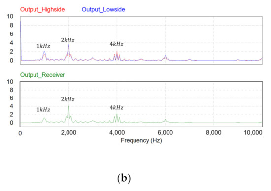
Figure 17.
Transmitter/receiver response characteristics (normal state): (a) transmitter/receiver frequency response; (b) transmitter/receiver FFT characteristics.
Figure 18 shows the response characteristics when a single signal from the high side or low side of the transmitter is input into the receiver owing to a disconnection in the PV system. In the FFT characteristics of Figure 18b,d, each frequency characteristic output from both sides of the transmitter appears in the receiver.
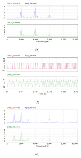
Figure 18.
Transmitter/receiver response characteristics (disconnection state): (a) high side frequency characteristics; (b) high side FFT characteristics; (c) low side frequency characteristics; (d) low side FFT characteristics.
In the circuit shown in Figure 16, disturbances of are input into the noise stage of the receiver. Figure 19 shows the response characteristics for this case.
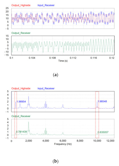
Figure 19.
Response characteristics to disturbances of the receiver: (a) frequency response characteristics to disturbance; (b) FFT characteristics for disturbance.
Table 2 shows a comparison of the input and output values of the receiver for the disturbance input. On comparing the receiver input and output for injected disturbance frequencies of 500 Hz and 10 kHz, the receiver output for disturbance was reduced by 61% and 68%, respectively, by the bandpass filter. This value exceeded the cut-off standard of 50%.
Table 2.
Input/output characteristics of the receiver against disturbance.
4.2. Result of the Experiments
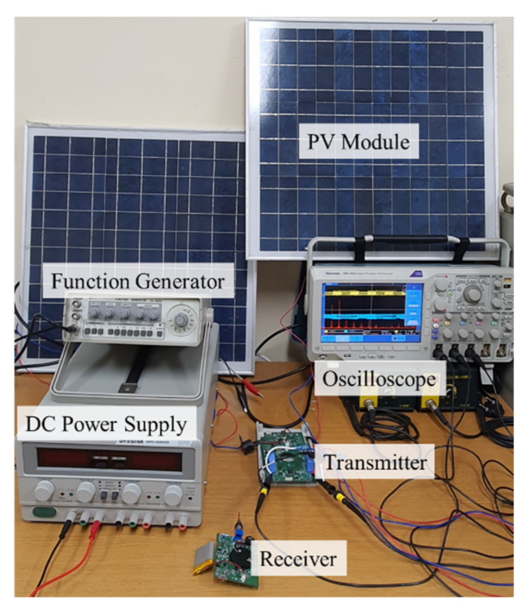
Figure 20 shows the experimental devices used to detect disconnection faults in PV systems. The devices used in the experiment were PV modules, an oscilloscope, a function generator, a power supply, a transmitter, and a receiver. Table 3 lists the specifications of the devices used in the experiment.

Figure 20.
Devices used in the experiments.
Table 3.
The experimental equipment’s specifications.
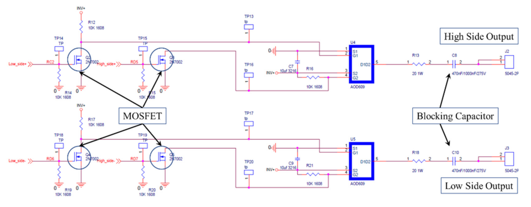
Figure 21 shows the transmitter’s frequency generation circuit for detecting the disconnection of the PV system, and Figure 22 shows the transmitter composed of PIC16F884 and 2N7002 (MOSFET). The red cable is the high side, outputting 4 and 2 kHz; the white cable is the low side, outputting 1 and 2 kHz; the black cable is a GND.
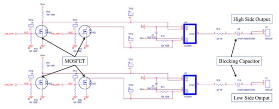
Figure 21.
Frequency generator circuit for the transmitter.
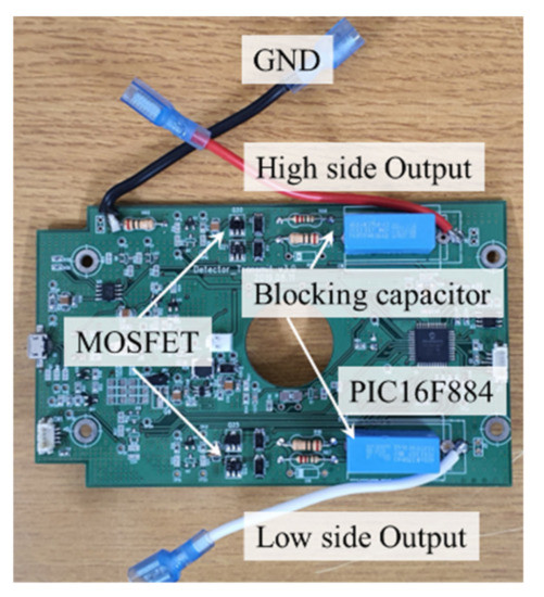
Figure 22.
Transmitter for disconnection detection.
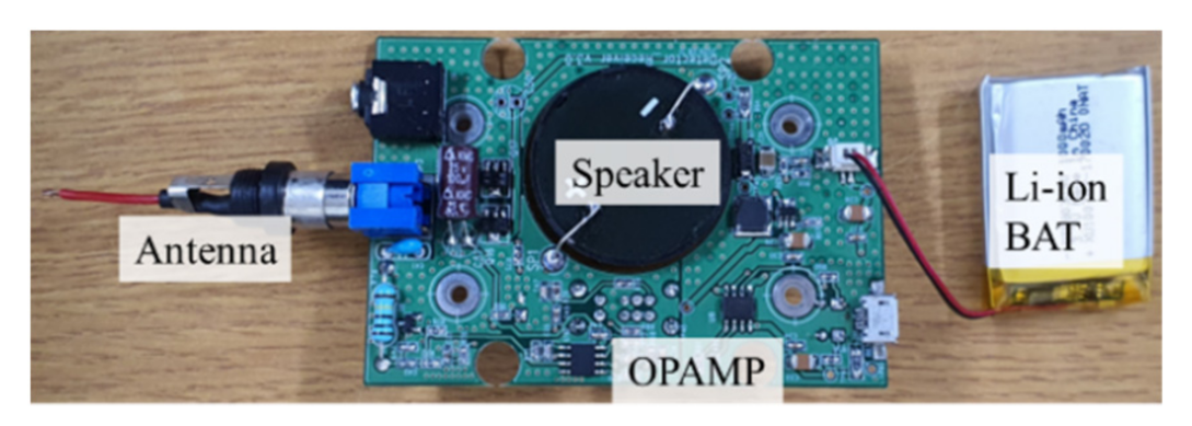
Figure 23 shows the receiver designed using the active filter of Figure 15. The active filter in the receiver used the LM741 OPAMP.

Figure 23.
Receiver for disconnection detection.
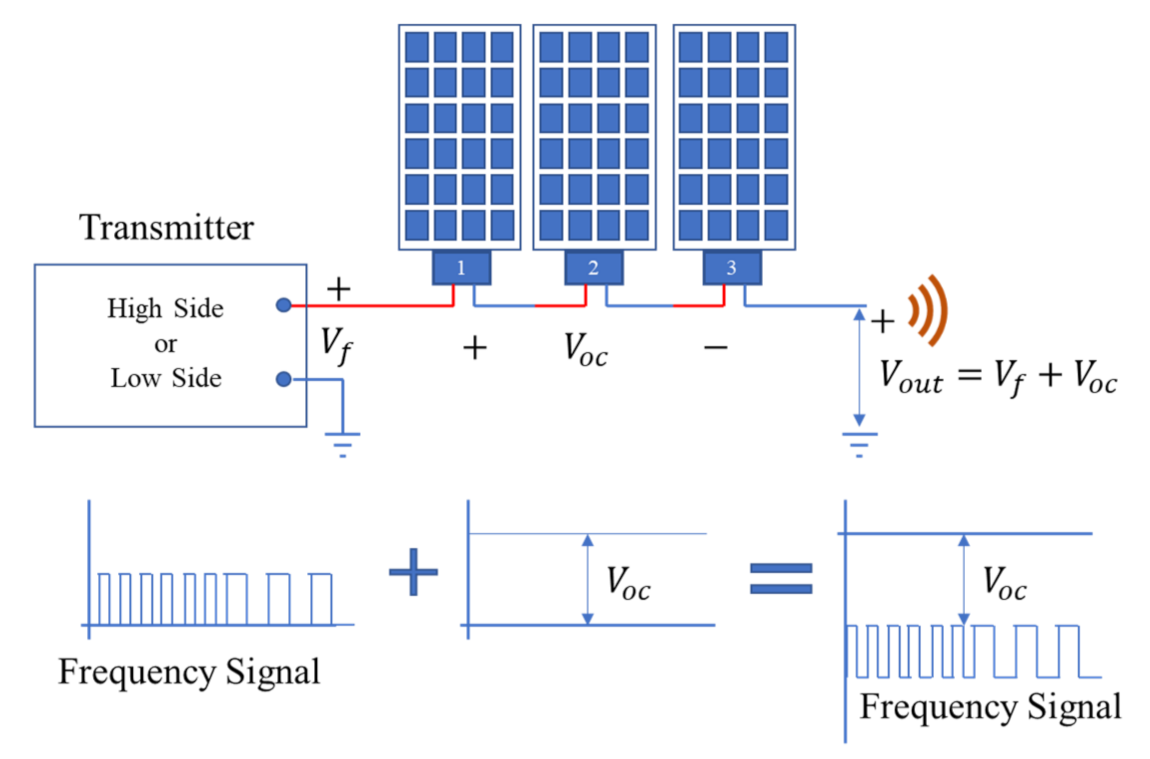
Figure 24 shows the process in which the injected signal of the transmitter is radiated at the point where the disconnection fault occurred. Because the signal of the transmitter injected into the PV string and the disconnection point are parallel connections, the signal radiated at the disconnection point is shifted to the magnitude of the open circuit voltage of the PV string. Therefore, the signal injected from the transmitter radiates the frequency signal of the input transmitter regardless of the number of module connections.
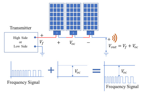
Figure 24.
Multiple frequency injection and radiation process.
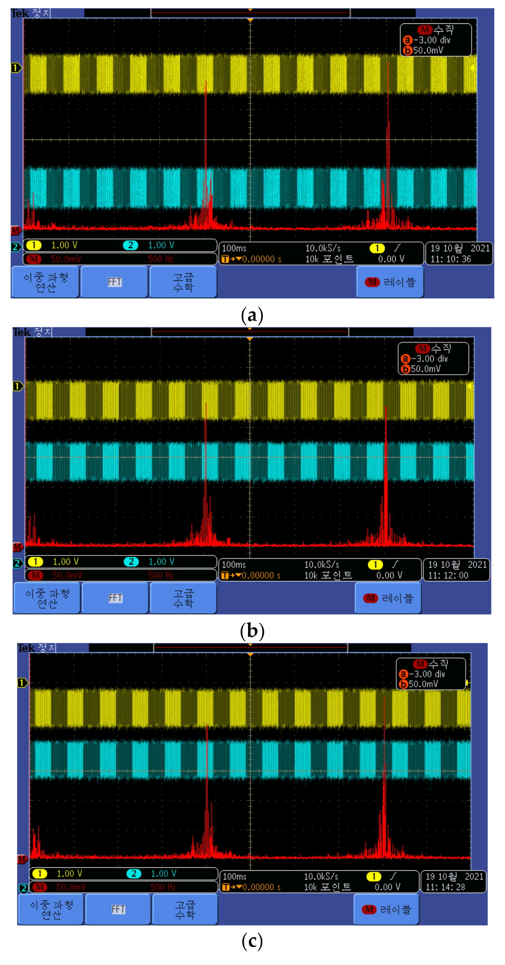
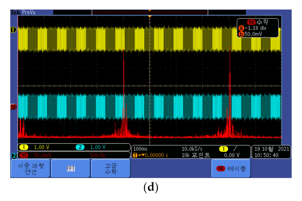
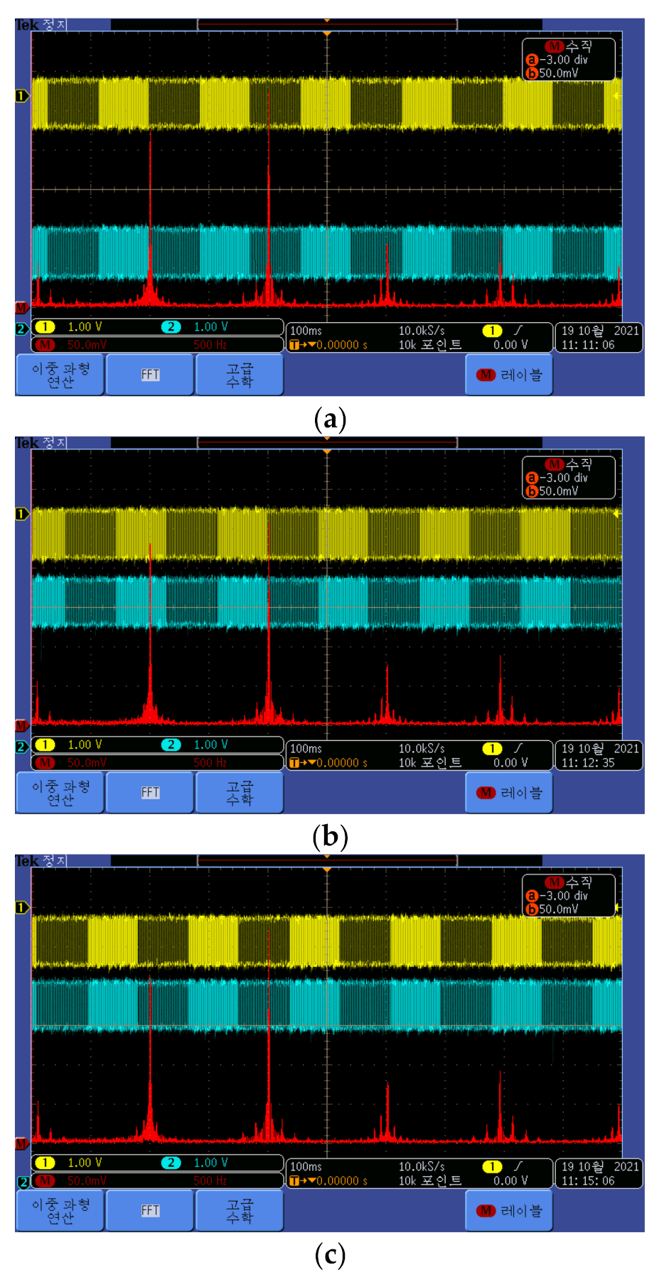
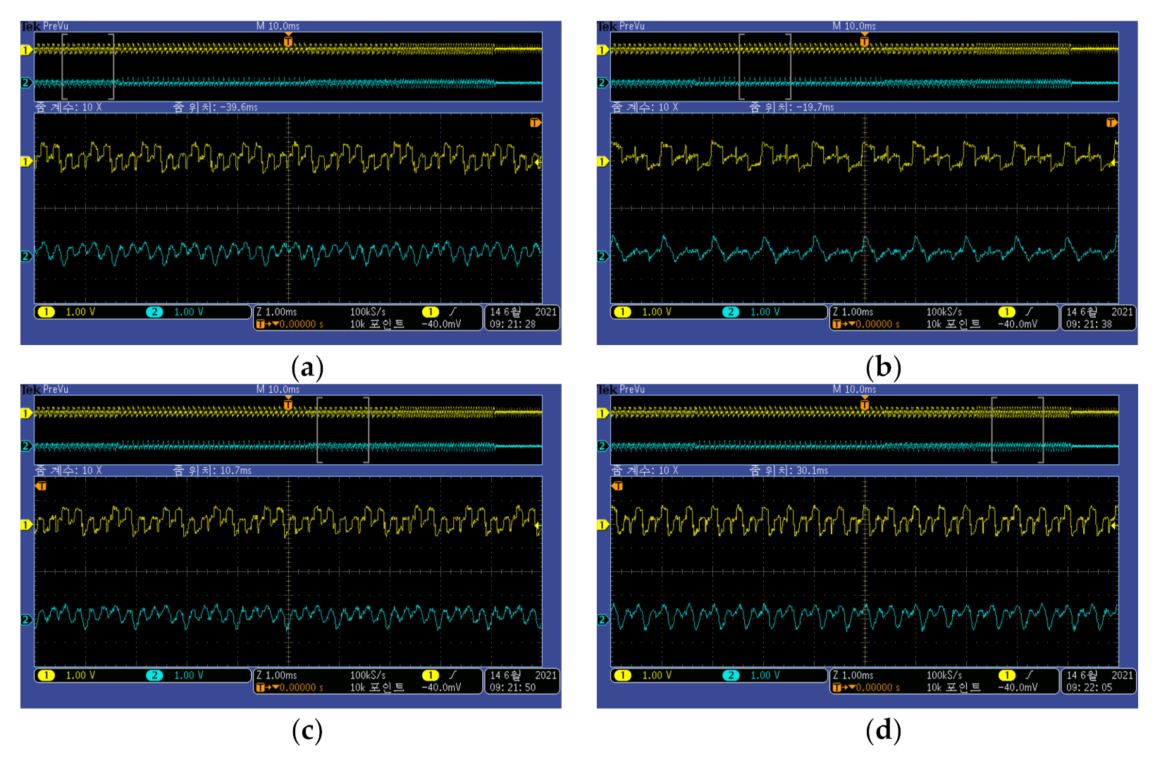
Figure 25 and Figure 26 show the characteristics of the PV module that passes the signals of the transmitter under changing numbers of PV modules in the PV string and operating conditions. For this experiment, the number of PV modules changed from one to three, and the operating conditions were good irradiation (outdoor) and bad irradiation (indoor). The high side and low side of the transmitter were connected to the positive pole terminal of the PV module, and the output of the negative pole terminal was measured using an oscilloscope. CH1 is the signal input into the PV module through the transmitter, and CH2 is the signal passed by the PV module. The red line shows the FFT characteristics of the CH2. In the results shown in Figure 25 and Figure 26, the values measured with the oscilloscope were similar when the number of modules and operating conditions were changed. Therefore, it can be confirmed that the frequency signal input from the transmitter passed the PV module owing to its capacitor factor, regardless of the number of PV modules and the operating conditions.
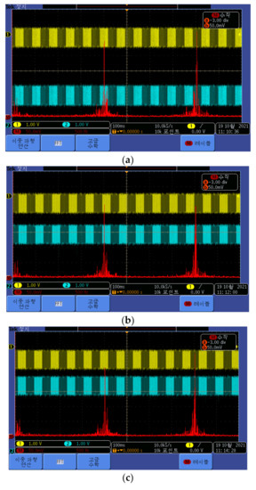

Figure 25.
Response characteristics according to the number of PV modules and the operating conditions (high side): (a) 1 module and good irradiation; (b) 2 modules and good irradiation; (c) 3 modules and good irradiation; (d) 3 modules and bad irradiation.
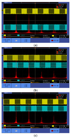

Figure 26.
Response characteristics according to the number of PV modules and the operating conditions (low side): (a) 1 module and good irradiation; (b) 2 modules and good irradiation; (c) 3 modules and good irradiation; (d) 3 modules and bad irradiation.
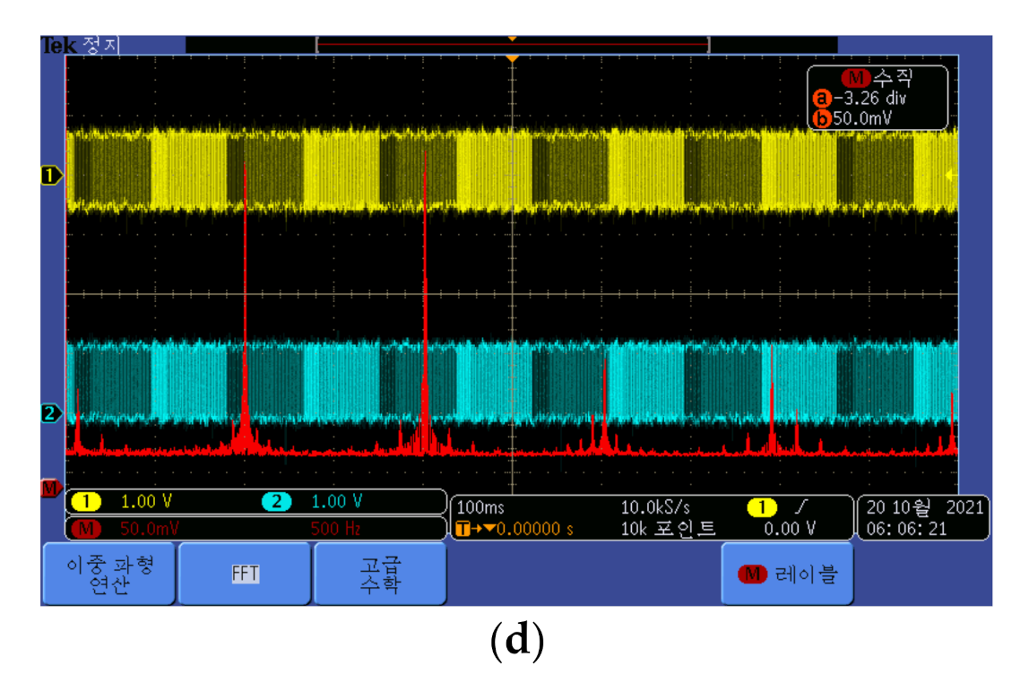
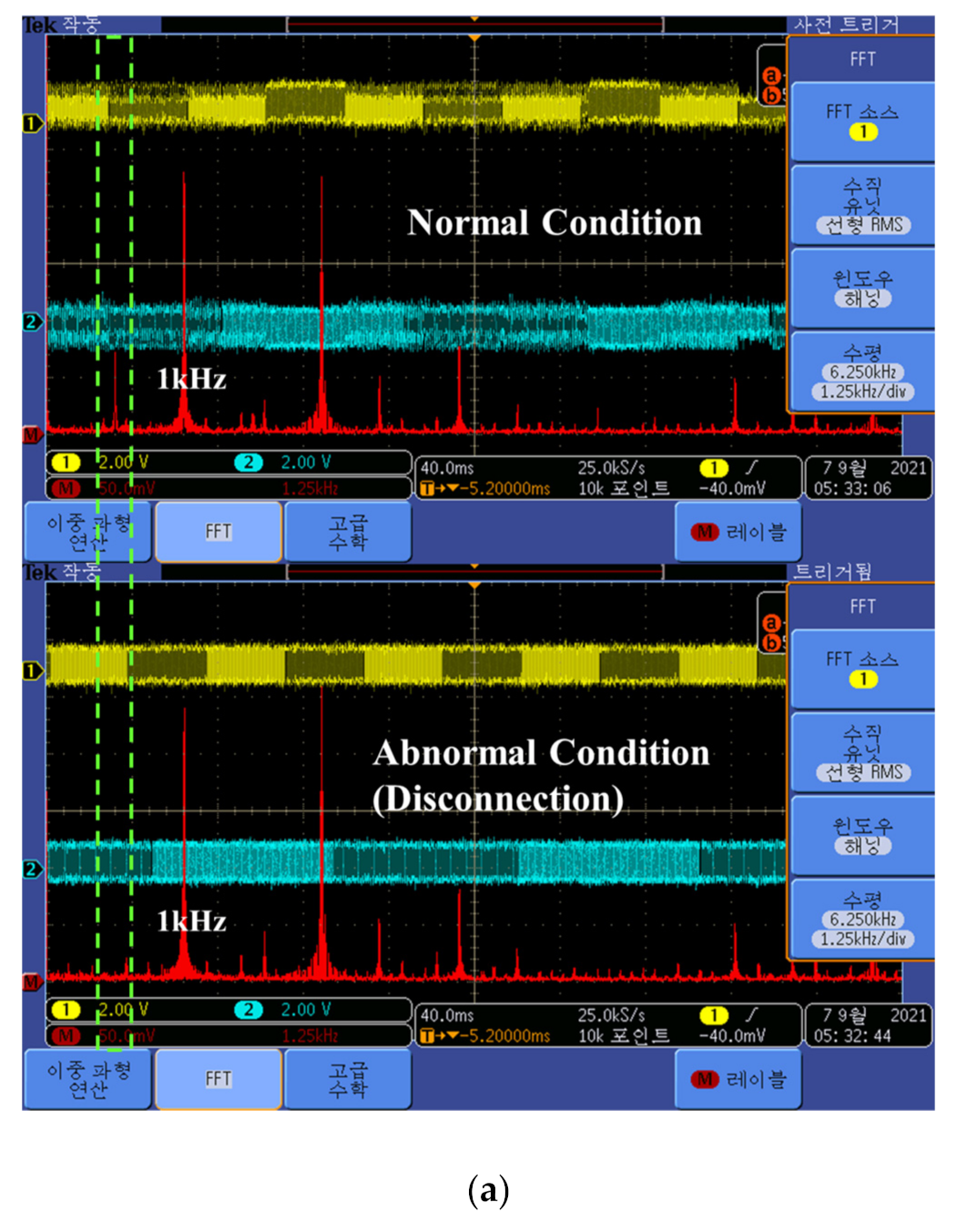
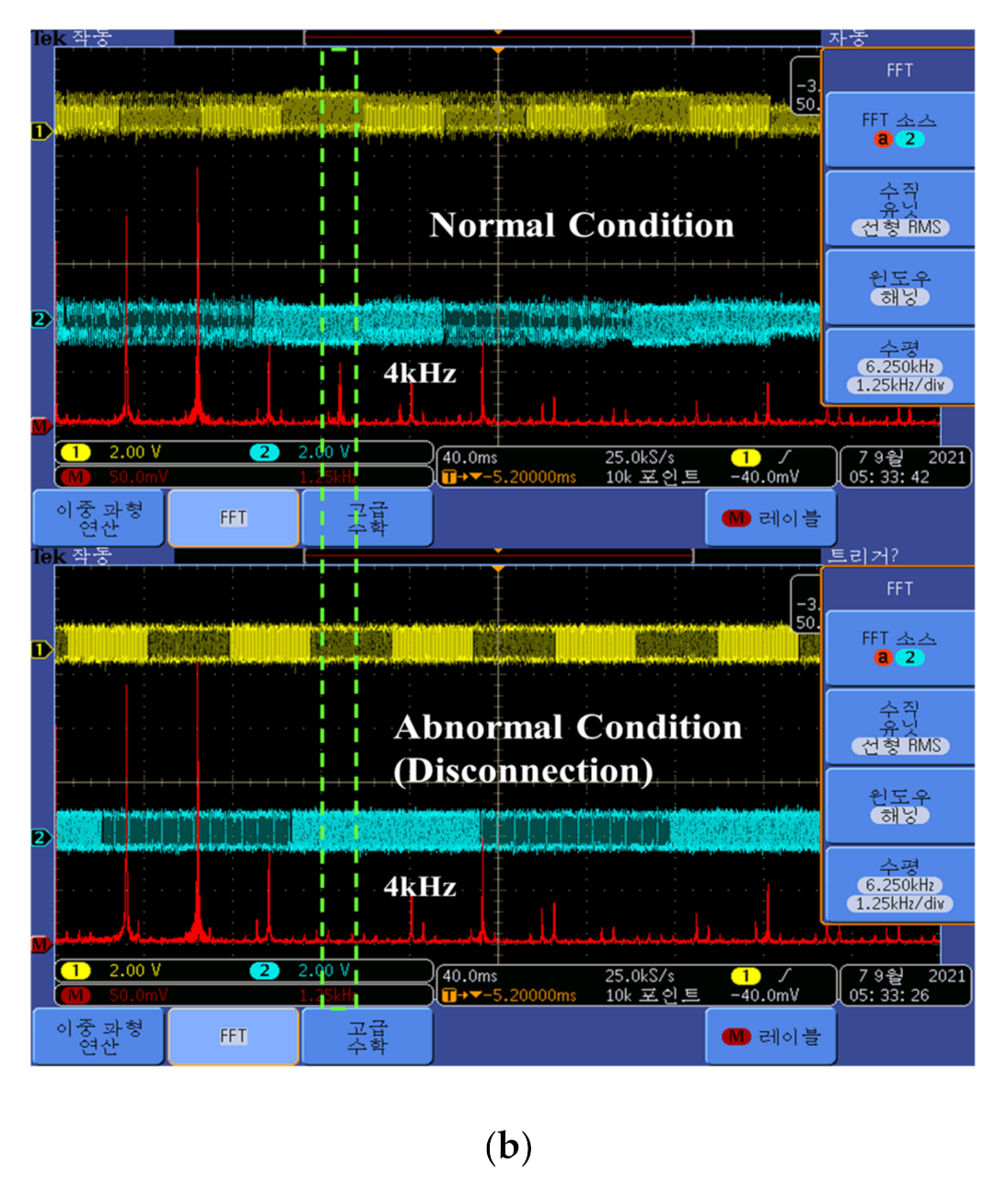
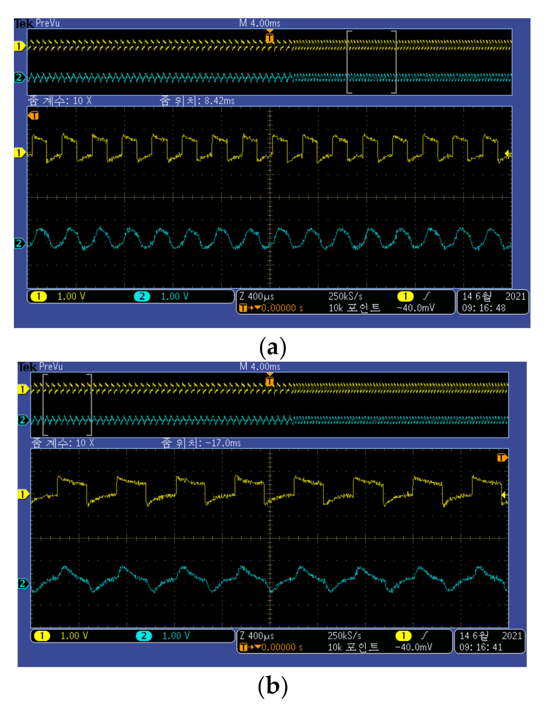
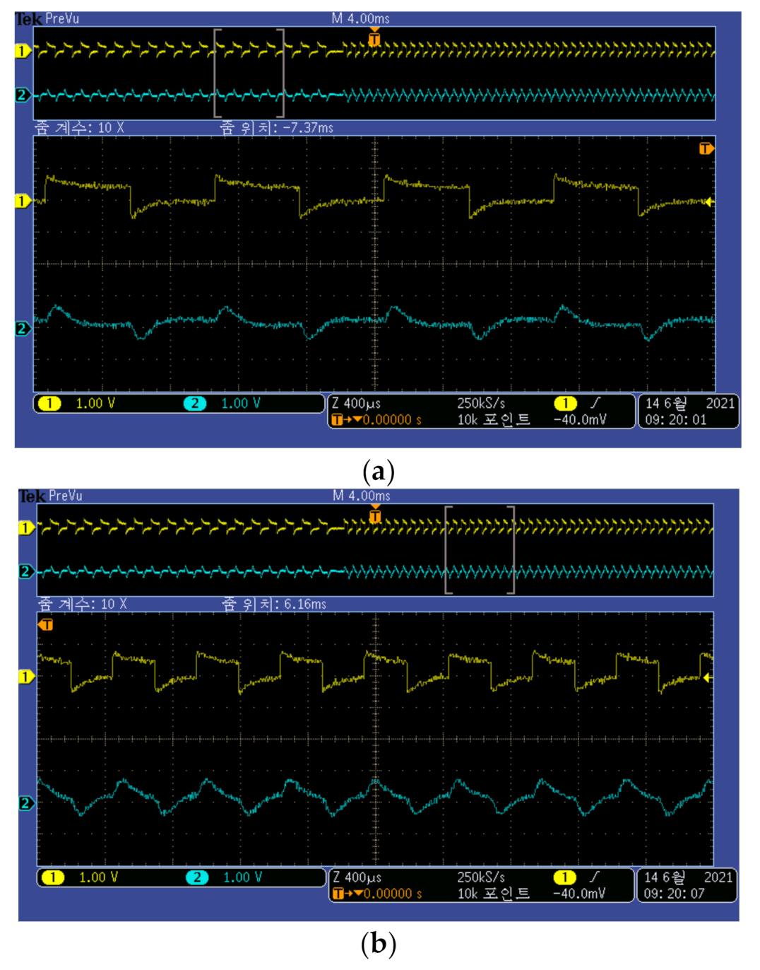
Figure 27 shows the characteristics when multiple frequencies are injected by connecting the high side to the +terminal of the PV module and the low side to the –terminal. CH1 is the high side frequency, CH2 is the low side frequency, and the red line shows the FFT characteristics. In Figure 27a, the high side outputs were 4 and 2 kHz, but when there was no disconnection (Figure 27a, top), a 1 kHz of low side frequency was included in the high side. In Figure 27b, in the normal state (Figure 27b, top), the 4 kHz of high side frequency was included in the FFT of the low side. When a disconnection fault occurred (Figure 27a,b, bottom), only the frequency components of the high side and low side were detected so that the disconnection could be confirmed.
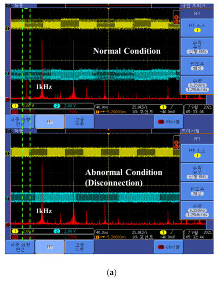

Figure 27.
Frequency and FFT characteristics according to the PV system’s operational status: (a) high side; (b) low side.
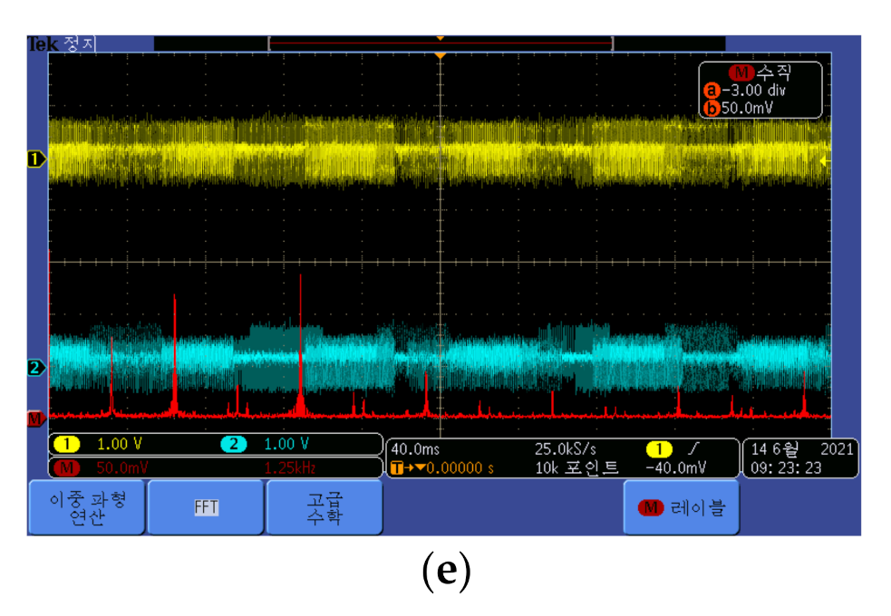
Figure 28 shows the overlapped characteristics of the high side frequency and the low side frequency of the transmitter in the normal state where no disconnection occurred. The frequency appeared according to the four output characteristics.
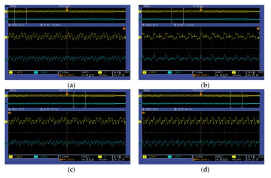

Figure 28.
Disconnection detector frequency characteristics under a normal state: (a) 4 + 1 kHz; (b) 2 + 1 kHz; (c) 4 + 2 kHz; (d) 2 + 2 kHz; (e) overall characteristics.
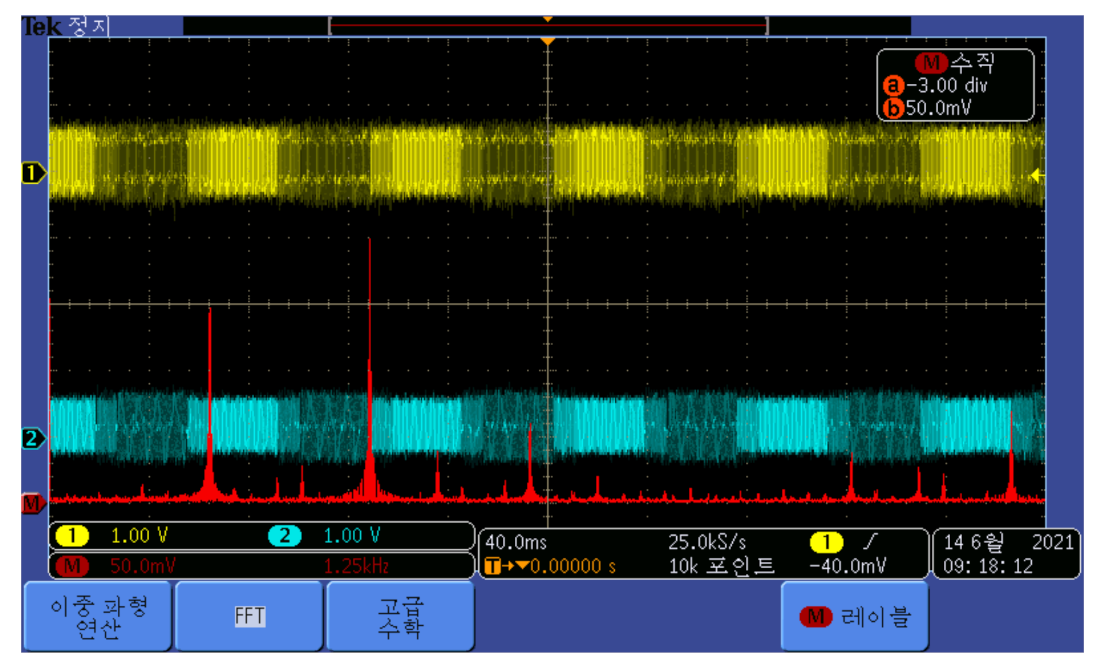
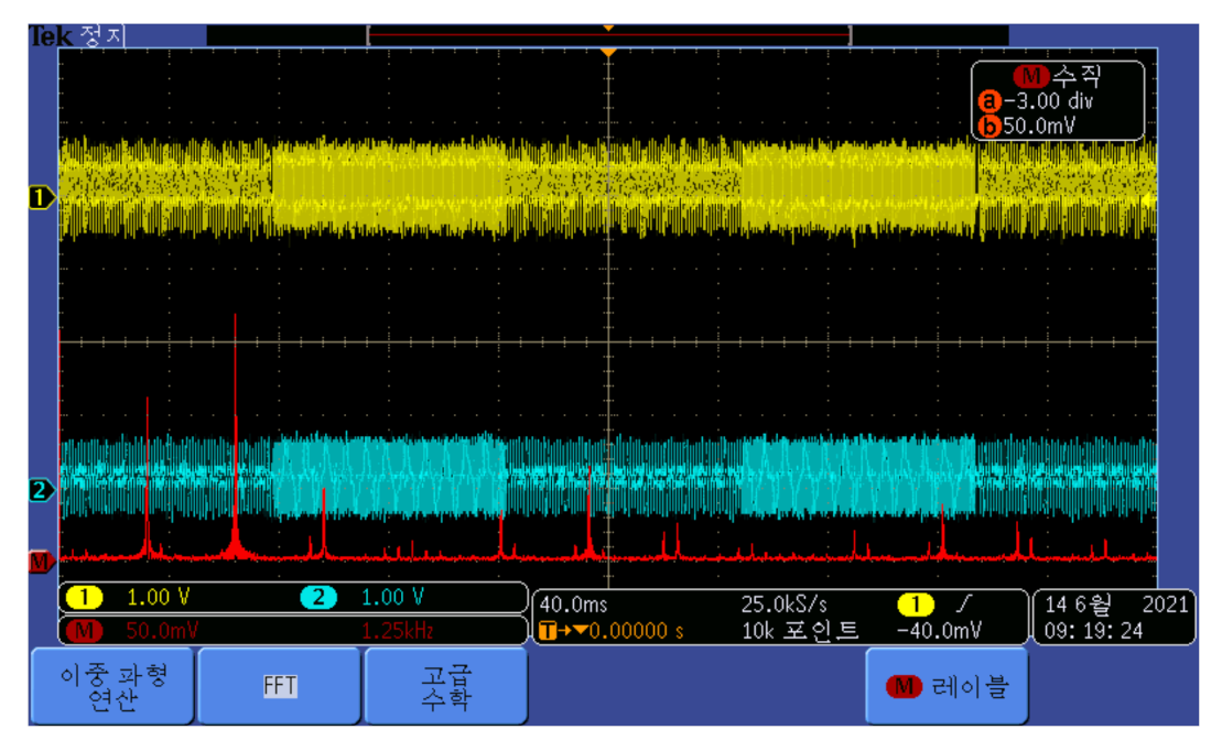
Figure 29 shows the characteristics when the receiver measures the frequency signal of the transmitter’s high side. CH1 is the output of the transmitter, and CH2 is the signal measured by the receiver. The red line is the FFT characteristic of the measurement signal of the receiver, and the transmitter’s high side frequency (4 and 2 kHz) was the highest. Figure 30 shows an expanded view of each frequency in Figure 29.
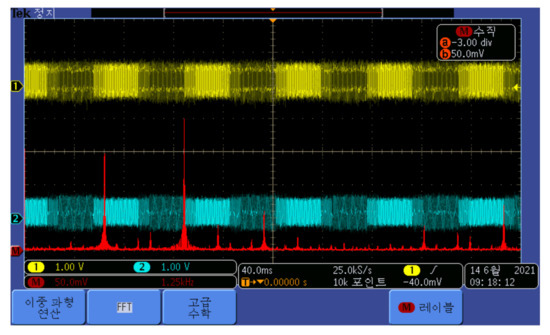
Figure 29.
Transmitter and receiver frequency characteristics (high side).

Figure 30.
Expansion of Figure 29: (a) 4 kHz region; (b) 2 kHz region.
Figure 31 shows the low side characteristics of the transmitter and receiver. CH1 is the low side output signal of the transmitter, and CH2 is the value measured through the receiver. The red line represents the FFT characteristic of CH2 (receiver). The 1 and 2 kHz, which are the frequencies of the transmitter’s low side, were the highest. Figure 32 shows an expanded view of each frequency part in Figure 31.

Figure 31.
Transmitter and receiver frequency characteristics (low side).
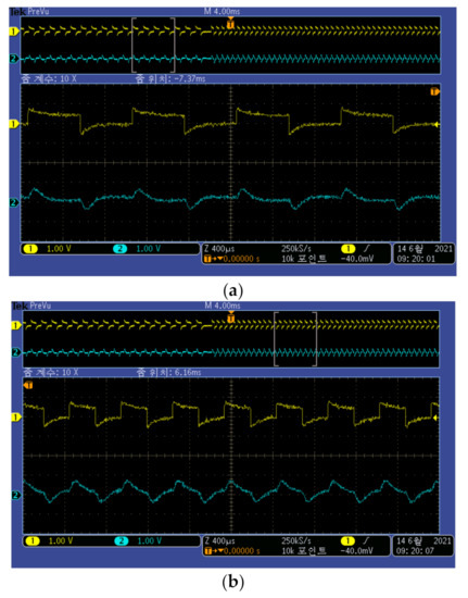
Figure 32.
Expansion of Figure 31: (a) 1 kHz region; (b) 2 kHz region.
According to the results analyzed in the simulations and experiments, the detected signal was different depending on whether there was a disconnection, so it was possible to determine the disconnection failure and the failure’s location.
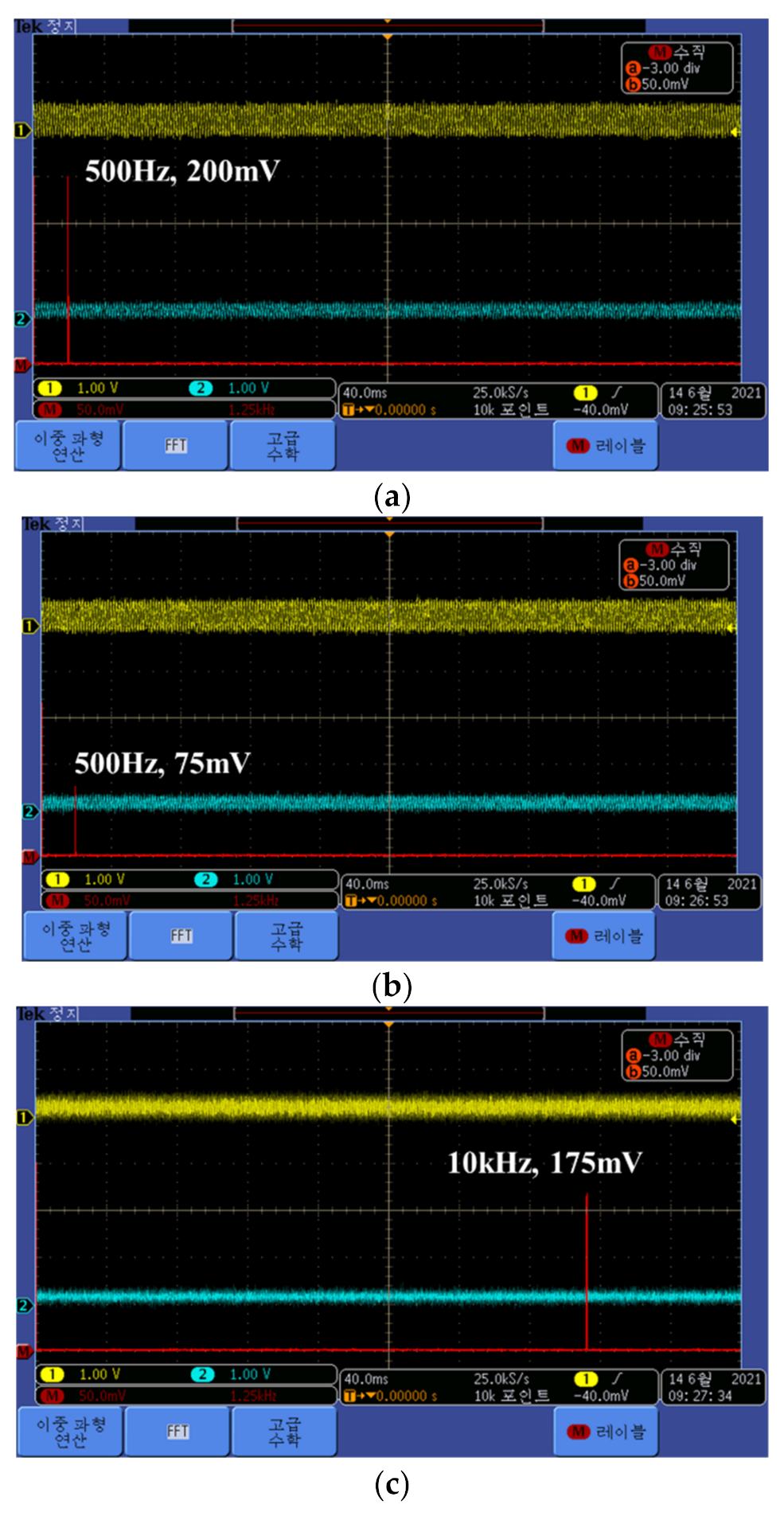
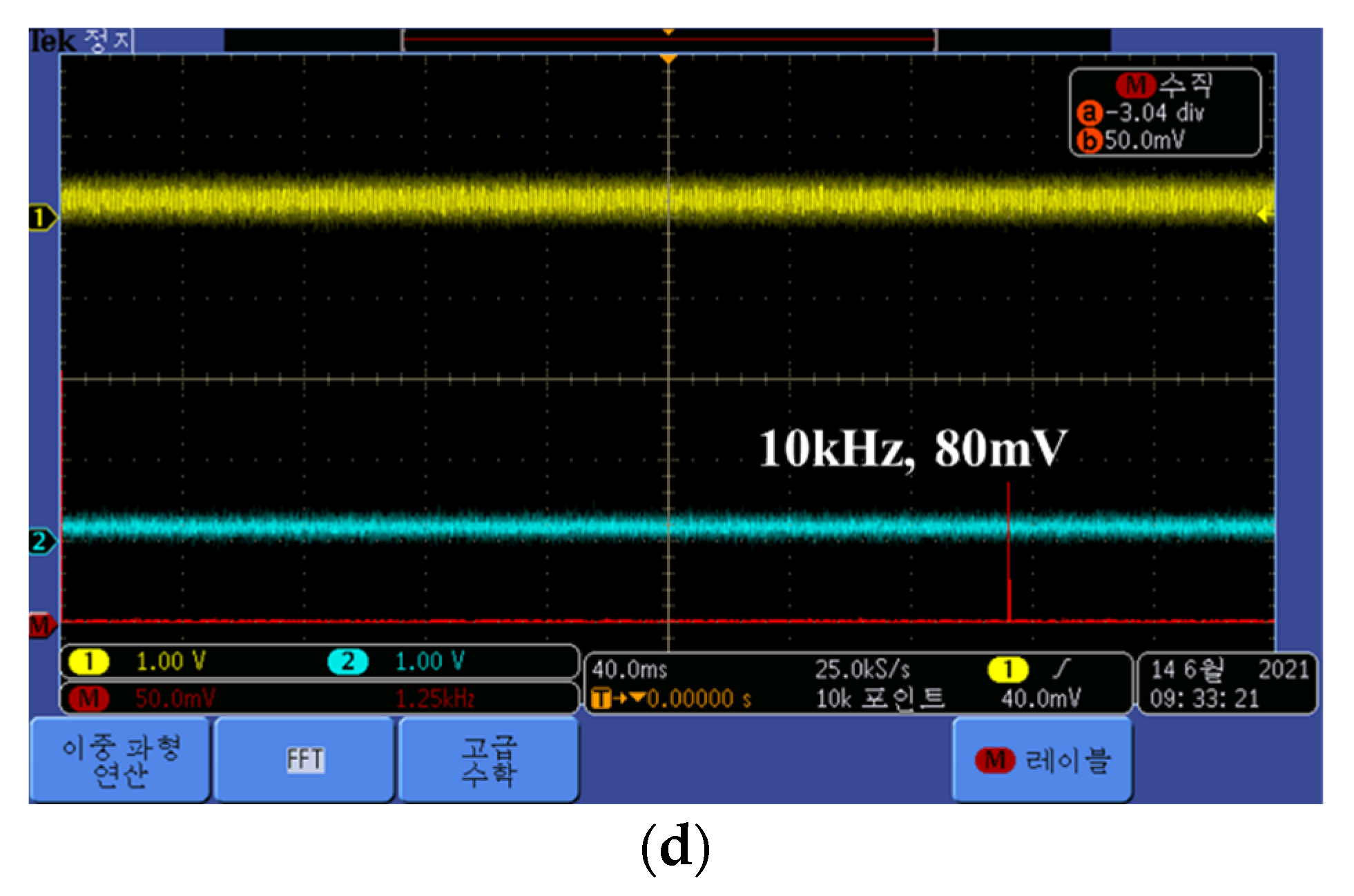
Figure 33 shows the blocking characteristics of the active filter of the receiver. The designed active filter was a band-pass filter that passed between 800a and 5300a Hz. To confirm the cut-off characteristics, 500 Hz and 10 kHz disturbances were injected into the receiver, and the characteristics of the injected signal were analyzed. Figure 33a shows the characteristics for a 500 Hz input. CH1 is the signal input into the active filter, CH2 is the signal passing through the active filter, and the red line is the FFT characteristic of CH1. In the FFT characteristic, the magnitude of the injected disturbance was approximately 200 mV. Figure 33b shows the output of the characteristics of the receiver for a 500 Hz disturbance. The red line is the FFT characteristic of CH2 with a size of 75 mV. Figure 33c shows the characteristics for a 10 kHz disturbance. The red line is the FFT characteristic for CH1, which input a 10 kHz disturbance, and the size was 175 mV. Figure 33d shows the output characteristics of the receiver when the 10 kHz disturbance passed the bandpass filter of the receiver. The red line is the FFT characteristic of CH2, which was a signal that passed through the filter of the receiver, and the size was approximately 80 mV. Table 4 shows a comparison of the input and output of the active filter and the damping ratio. The 500 Hz and 10 kHz disturbances outside the passing region of the designed active filter were reduced by 62.5% and 54.3%, respectively, exceeding the cut-off standard of 50%. Therefore, the disturbance of the receiver was removed by the designed filter.

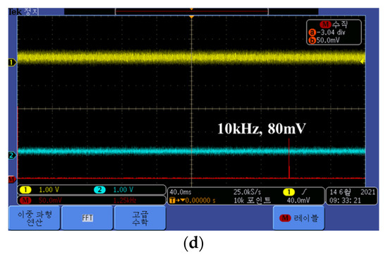
Figure 33.
Receiver response characteristics regarding disturbance: (a) 500 Hz input; (b) 500 Hz output; (c) 10 kHz input; (d) 10 kHz output.
Table 4.
Comparison of the response characteristics to disturbance.
5. Conclusions
This paper presented a method to exactly and simply detect disconnection faults and fault locations in PV systems using multiple frequency injection. To detect the disconnection failure of PV systems, the method presented in this paper used the characteristics in which the AC equivalent circuit of a solar cell had a parallel capacitor. Because the capacitor had the characteristic of passing AC signals well, we designed a transmitter that included a high side using 4 and 2 kHz and a low side using 1 and 2 kHz. The transmitter was connected to the PV array or PV string, and multiple frequencies were injected into both terminals. By analyzing the characteristics of the injected signal, disconnection faults and fault locations were detected. When disconnection failure occurred, the disconnection point operated as an antenna and radiated the injected signal to the outside. This externally radiated signal could be detected by a receiver with a band-pass filter that passed only a specific frequency band, and the exact disconnection position could be determined according to the pattern of the detected signal.
The proposed method analyzed the frequency transmission characteristics through the PV module, the output signal of the transmitter, and the input signal of the receiver. With no disconnection, the frequencies’ output to the transmitter overlapped, and when disconnection occurred, only the signals injected from the high side and low side of the transmitter appeared. The receiver, which detected the signal injected into the transmitter, was designed as a band-pass filter using an active filter to detect only the injected signal. The method proposed in this paper can easily find the disconnection failure of a PV system. However, this method injects a signal into both ends of the PV string when a disconnection fault occurs, and the user has to find the fault point by themselves. In addition, this paper was based on the case where there was only one disconnection fault, and additional research is needed on the occurrence of disconnection failure at multiple points.
This method presented in this paper can be used to detect failures, such as disconnection and deterioration of various conductors, and we will research it can be applied to various fields or multiple disconnection faults.
Author Contributions
Conceptualization, J.-S.K. and D.-K.K.; Data Curation, J.-S.K.; Formal Analysis, J.-S.K.; Funding Acquisition, D.-K.K.; Investigation, J.-S.K.; Methodology, D.-K.K.; Project Administration, D.-K.K.; Resources, J.-S.K.; Software, J.-S.K. and D.-K.K.; Supervision, D.-K.K.; Validation, D.-K.K.; Visualization, J.-S.K.; Writing—Original Draft, J.-S.K. and D.-K.K.; Writing—Review and Editing, D.-K.K. All authors have read and agreed to the published version of the manuscript.
Funding
This work was supported by the Gwangju Jeonnam local EnergyCluster Human Resources Development of the Korea Insitute of Energy Technology Evaluation and Planning (KETEP) grant funded by the Korea government Ministry of Knowledge Economy (No. 20214000000560).
Institutional Review Board Statement
Not applicable.
Informed Consent Statement
Not applicable.
Data Availability Statement
Not applicable.
Conflicts of Interest
The authors declare no conflict of interest.
References
- Pathway to Critical and Formidable Goal of Net-Zero Emissions by 2050 is Narrow but Brings Huge Benefits, According to IEA Special Report. Available online: https://www.iea.org/news/pathway-to-critical-and-formidable-goal-of-net-zero-emissions-by-2050-is-narrow-but-brings-huge-benefits (accessed on 8 September 2021).
- Understanding PV System Losses, Part 1: Nameplate, Mismatch, and LID Losses. Available online: https://www.aurorasolar.com/blog/understanding-pv-system-losses-part-1/ (accessed on 8 September 2021).
- Eltawil, M.A.; Zhao, Z. Grid-connected photovoltaic power systems: Technical and potential problems—A review. Renew. Sustain. Energy Rev. 2010, 14, 112–129. [Google Scholar] [CrossRef]
- Ropp, M.E.; Begovic, M.; Rohatgi, A. Prevention of islanding in grid-connected photovoltaic systems. Prog. Photovolt. Res. Appl. 1999, 7, 39–59. [Google Scholar] [CrossRef]
- Connecting Solar Panels Together. Available online: https://www.alternative-energy-tutorials.com/solar-power/connecting-solar-panels-together.html (accessed on 8 September 2021).
- Pendem, S.R.; Mikkili, S. Performance evaluation of series, series-parallel and honey-comb PV array configurations under partial shading conditions. In Proceedings of the 2017 7th International Conference on Power Systems (ICPS), Shivajinagar, India, 21–23 December 2017; pp. 749–754. [Google Scholar] [CrossRef]
- Mehiri, A.; Hamid, A.; Almazrouei, S. The Effect of Shading with Different PV Array Configurations on the Grid-Connected PV System. In Proceedings of the 2017 International Renewable and Sustainable Energy Conference (IRSEC), Tangier, Morocco, 4–7 December 2017; pp. 1–6. [Google Scholar] [CrossRef]
- Hashunao, S.; Mehta, R.K. Fault Analysis of Solar Photovoltaic System. In Proceedings of the 2020 5th International Conference on Renewable Energies for Developing Countries (REDEC), Marrakech, Morocco, 24–26 March 2020; pp. 1–6. [Google Scholar] [CrossRef]
- Zhao, Y.; de Palma, J.; Mosesian, J.; Lyons, R.; Lehman, B. Line–Line Fault Analysis and Protection Challenges in Solar Photovoltaic Arrays. IEEE Trans. Ind. Electron. 2013, 60, 3784–3795. [Google Scholar] [CrossRef]
- Saleh, M.U.; Deline, C.; Kingston, S.; Jayakumar, N.K.T.; Benoit, E.; Harley, J.B.; Furse, C.; Scarpulla, M. Detection and Localization of Disconnections in PV Strings Using Spread-Spectrum Time-Domain Reflectometry. IEEE J. Photovolt. 2020, 10, 236–242. [Google Scholar] [CrossRef]
- Roman, E.; Alonso, R.; Ibanez, P.; Elorduizapatarietxe, S.; Goitia, D. Intelligent PV Module for Grid-Connected PV Systems. IEEE Trans. Ind. Electron. 2006, 53, 1066–1073. [Google Scholar] [CrossRef]
- Tsanakas, J.A.; Ha, L.; Buerhop, C. Faults and infrared thermographic diagnosis in operating c-Si photovoltaic modules: Areviewof research and future challenges. Renew. Sustain. Energy Rev. 2016, 62, 695–709. [Google Scholar] [CrossRef]
- Mellit, A.; Tina, G.M.; Kalogirou, S.A. Fault detection and diagnosis methods for photovoltaic systems: A review. Renew. Sustain. Energy Rev. 2018, 91, 1–17. [Google Scholar] [CrossRef]
- Quater, P.B.; Grimaccia, F.; Leva, S.; Mussetta, M.; Aghaei, M. Light Unmanned Aerial Vehicles (UAVs) for Cooperative Inspection of PV Plants. IEEE J. Photovolt. 2014, 4, 1107–1113. [Google Scholar] [CrossRef] [Green Version]
- Triki-Lahiani, A.; Abdelghani, A.B.-B.; Slama-Belkhodja, I. Fault detection and monitoring systems for photovoltaic installations: A review. Renew. Sustain. Energy Rev. 2018, 82, 2680–2692. [Google Scholar] [CrossRef]
- Furse, C.; Chung, Y.C.; Lo, C.; Pendayala, P. A critical comparison of reflectometry methods for location of wiring faults. Smart Struct. Syst. 2006, 2, 25–46. [Google Scholar] [CrossRef] [Green Version]
- Takashima, T.; Yamaguchi, J.; Otani, K.; Oozeki, T.; Kato, K.; Ishida, M. Experimental studies of fault location in PV module strings. Sol. Energy Mater. Sol. Cells 2009, 93, 1079–1082. [Google Scholar] [CrossRef]
- Zhang, J.; Zhang, Y.; Guan, Y. Analysis of time-domain reflectometry combined with wavelet transform for fault detection in aircraft shielded cables. IEEE Sens. J. 2016, 16, 4579–4586. [Google Scholar] [CrossRef]
- Kumar, R.A.; Suresh, M.S.; Nagaraju, J. Silicon (BSFR) solar cell AC parameters at different temperatures. Sol. Energy Mater. Sol. Cells 2005, 85, 397–406. [Google Scholar] [CrossRef]
- El-Maksood, A.M.A. Performance Dependence of (I-V) and (C-V) for Solar Cells on Environmental Conditions. J. Adv. Phys. 2018, 14, 5331–5351. [Google Scholar] [CrossRef]
- Harper, J.; Wang, X.I. CV and AC Impedance Techniques and Characterizations of Photovoltaic Cells. Available online: https://file.scirp.org/pdf/22-1.476.pdf (accessed on 9 September 2021).
- Kumar, S.; Sareen, V.; Batra, N.; Singh, P.K. Study of C–V characteristics in thin n+-p-p+ silicon solar cell sand induced junction n-p-p+ cell structures. Sol. Energy Mater. Sol. Cells 2010, 94, 1469–1472. [Google Scholar] [CrossRef]
- Kumar, S.; Singh, P.K.; Chilana, G.S. Study of silicon solar cell at different intensities of illumination and wavelengths using impedance spectroscopy. Sol. Energy Mater. Sol. Cells 2009, 93, 1881–1884. [Google Scholar] [CrossRef]
- Burgelman, M.; Nollet, P. Admittance spectroscopy of thin film solar cells. Solid State Ion. 2005, 176, 2171–2175. [Google Scholar] [CrossRef]
- Bayhan, H.; Kavasoˇglu, A.S. Admittance and Impedance Spectroscopy on Cu(In,Ga)Se2 Solar Cells. Turk. J. Phys. 2003, 27, 529–535. [Google Scholar]
- Kumar, R.A.; Suresh, M.S.; Nagaraju, J. GaAs/Ge solar cell AC parameters under illumination. Sol. Energy 2004, 76, 417–421. [Google Scholar] [CrossRef]
- Panigrahi, J.; Singh, R.; Batra, N.; Gope, J.; Sharma, M.; Pathi, P.; Srivastava, S.K.; Rauthan, C.M.S.; Singh, P.K. Impedance spectroscopy of crystalline silicon solar cell: Observation of negative capacitance. Sol. Energy 2016, 136, 412–420. [Google Scholar] [CrossRef]
- Mandal, H.; Nagaraju, J. GaAs/Ge and silicon solar cell capacitance measurement using triangular wave method. Sol. Energy Mater. Sol. Cells 2007, 91, 696–700. [Google Scholar] [CrossRef]
- Anantha Krishna, H.; Misra, N.K.; Suresh, M.S. Use of solar cells for measuring temperature of solar cell blanket in spacecrafts. Sol. Energy Mater. Sol. Cells 2012, 102, 184–188. [Google Scholar] [CrossRef]
- Principles of Communication—FM Radio. Available online: https://www.tutorialspoint.com/principles_of_communication/principles_of_communication_fm_radio.htm (accessed on 9 September 2021).
- Zhao, Y. Fault Analysis in Solar Photovoltaic Arrays. Ph.D. Thesis, Northeastern University, Boston, MA, USA, 2011. [Google Scholar]
- Trejos-Grisales, L.A.; Bastidas-Rodríguez, J.D.; Ramos-Paja, C.A. Mathematical Model for Regular and Irregular PV Arrays with Improved Calculation Speed. Sustainability 2020, 12, 10684. [Google Scholar] [CrossRef]
- Lillo-Bravo, I.; González-Martínez, P.; Larrañeta, M.; Guasumba-Codena, J. Impact of Energy Losses Due to Failures on Photovoltaic Plant Energy Balance. Energies 2018, 11, 363. [Google Scholar] [CrossRef] [Green Version]
- Cotfas, P.A.; Cotfas, D.T.; Borza, P.N.; Sera, D.; Teodorescu, R. Solar Cell Capacitance Determination Based on an RLC Resonant Circuit. Energies 2018, 11, 672. [Google Scholar] [CrossRef] [Green Version]
- Cotfas, D.T.; Cotfas, P.A.; Kaplanis, S. Methods and techniques to determine the dynamic parameters of solar cells: Review. Renew. Sustain. Energy Rev. 2016, 61, 213–221. [Google Scholar] [CrossRef]
- Yadav, P.; Pandey, K.; Bhatt, V.; Kumar, M.; Kim, J. Critical aspects of impedance spectroscopy in silicon solar cell characterization: A review. Renew. Sustain. Energy Rev. 2017, 76, 1562–1578. [Google Scholar] [CrossRef]
- Raj, S.; Kumar, S.A.; Panchal, A.K. Solar cell parameters estimation from illuminated I-V characteristic using linear slope equations and Newton-Raphson technique. J. Renew. Sustain. Energy 2013, 5, 255–265. [Google Scholar] [CrossRef]
- Cubas, J.; Pindado, S.; De Manuel, C. Explicit Expressions for Solar Panel Equivalent Circuit Parameters Based on Analytical Formulation and the Lambert W-Function. Energies 2014, 7, 4098–4115. [Google Scholar] [CrossRef] [Green Version]
- Mughal, M.A.; Ma, Q.; Xiao, C. Photovoltaic Cell Parameter Estimation Using Hybrid Particle Swarm Optimization and Simulated Annealing. Energies 2017, 10, 1213. [Google Scholar] [CrossRef] [Green Version]
- Ye, M.; Wang, X.; Xu, Y. Parameter extraction of solar cells using particle swarm optimization. J. Appl. Phys. 2009, 105, 094502. [Google Scholar] [CrossRef]
- Zagrouba, M.; Sellami, A.; Bouaïcha, M.; Ksouri, M. Identification of PV solar cells and modules parameters using the genetic algorithms: Application to maximum power extraction. Sol. Energy 2010, 84, 860–866. [Google Scholar] [CrossRef]
- Hasanien, H.M. Shuffled Frog Leaping Algorithm for Photovoltaic Model Identification. IEEE Trans. Sustain. Energy 2015, 6, 509–515. [Google Scholar] [CrossRef]
- Yu, K.; Chen, X.; Wang, X.; Wang, Z. Parameters identification of photovoltaic models using self-adaptive teaching-learning-based optimization. Energy Convers. Manag. 2017, 145, 233–246. [Google Scholar] [CrossRef]
- Stošović, M.A.; Lukač, D.; Litovski, I.; Litovski, V. Frequency domain characterization of a solar cell. In Proceedings of the 11th Symposium on Neural Network Applications in Electrical Engineering, Belgrade, Serbia, 20–22 September 2012; pp. 259–264. [Google Scholar] [CrossRef]


Publisher’s Note: MDPI stays neutral with regard to jurisdictional claims in published maps and institutional affiliations. |
© 2021 by the authors. Licensee MDPI, Basel, Switzerland. This article is an open access article distributed under the terms and conditions of the Creative Commons Attribution (CC BY) license (https://creativecommons.org/licenses/by/4.0/).