Abstract
In a competitive electricity market, both electricity retailers and generators predict future prices and volumes and execute electricity delivery contracts through power exchange. In such circumstances, they may suffer from uncertainties caused by fluctuations in spot prices and future demand due to their high volatility. In this study, we develop a unified approach using derivatives and forwards on the spot electricity price and weather data to mitigate the cashflow fluctuation for power utilities. We aim to clarify the applicability of our proposed methods and provide a new and useful perspective on hedging schemes involving various electricity utilities, such as power retailers, solar photovoltaic (PV) generators, and thermal generators. Moreover, we analyze the risk of risk takers (such as the insurance companies in this study) in the derivatives market. In addition, we perform empirical simulations to measure out-of-sample hedging effects on their cashflow management using actual data in Japan.
1. Introduction
In electricity markets, the transactions of electricity delivery contracts between power retailers and generators are based on predictions of demand and supply that reflect the actual consumption of the end-users as well as the renewable power generation in the future. For example, the demand volume for power retailers largely depends on the future temperature, whereas the power output from solar photovoltaic (PV) and other renewable energy generation fluctuates over time according to the future weather conditions. In addition, energy prices, such as oil and natural gas, affect the electricity price as well as the supply and demand predictions, and so the spot electricity price is quite volatile in a competitive power exchange market. In such a situation, power retailers and generators suffer from the risk of simultaneous price and volume fluctuations, leading to large volatility in their cashflows, and adequate strategies for reducing the cashflow fluctuations are required for power utilities. Therefore, financial instruments, including derivatives and forwards on spot electricity prices and weather indexes, are considered effective tools [1,2].
There are several previous studies on electricity derivatives and weather derivatives, and various methods that have been proposed, especially in the context of pricing. For electricity derivatives, there is a relatively wide variety of studies on the pricing of option-type derivatives (e.g., [3,4,5,6]), which are systematically reviewed in [1]. Other characteristic-related works include, for example, Oum et al. [7], who proposed an expected utility-based approach for constructing electricity derivatives with arbitrary nonlinear payoff functions. Recently, there have been pricing methods for electricity derivatives with various granularities and payoffs, such as “cap/floor futures”, where the underlying asset is the hourly intraday electricity price, traded on a weekly basis [8], and “day-ahead cap futures” with the day-ahead price as the underlying asset, traded on a daily basis [9].
As for weather derivatives, various studies have been carried out, mainly on pricing methods. There are a wide range of indices that can be used as underlying assets for weather derivatives, such as temperature [10,11,12,13,14,15,16,17,18,19,20], wind [21,22,23,24], solar radiation [25], and rainfall [26]; thus, the applicability of weather derivatives has been demonstrated by many researchers. Recently, the research on the investigation of hedging effects has gained attention as well. As an example of such previous studies, Bhattacharya et al. [27] have illustrated the hedging effect of weather derivatives (using heating degree days (HDDs) and cooling degree days (CDDs)) on the profit fluctuations of a solar PV generator using a data-driven approach.
Instead of applying standard derivatives, unique derivatives based on nonparametric regression techniques have been proposed to further improve the hedging effectiveness [28,29,30,31,32,33,34]. The approach of those studies is to estimate the nonlinear functions of the optimal payoffs and/or the optimal contract volumes of the derivatives using generalized additive models (GAMs [35,36]). That is, those studies focus on, for example, the fact that price volatility can lead to losses for retail businesses that sell electricity at fixed prices [31] and clarify the importance and effectiveness of strategies to effectively suppress fluctuations in cash flows. Among them, our recent study [33] has demonstrated that derivatives based on temperature and solar radiation are highly effective in hedging the risk of revenue fluctuations for electricity retailers and solar PV generators, and a more recent study [34] has focused on the methodological refinement of the choice of spline basis functions.
In this study, we systematically organize the theoretical aspects of our previous studies [33,34] to develop a unified approach using electricity and weather derivatives/forwards and demonstrate a comprehensive analysis of various types of players. We aim to not only to clarify the applicability of our proposed methods, but also to provide a new and useful perspective on derivative trading schemes involving different electricity utilities and insurance companies. In our empirical analysis, we assume three types of players—electricity retailers, solar PV generators, and thermal power generators—and measure the hedging effects on their cashflow management using electricity and weather derivatives (as well as forward contracts). What is unique about this study is that we deal with “forwards” with linear payoffs as well as “derivatives” with nonlinear payoffs for three different types of electricity businesses and compare the hedging effects (and hedging errors) of both types of hedge instruments from various perspectives. In addition, we apply the methodology of previous studies on daily granular derivative contracts [33,34] to derivatives with hourly granularity payoffs and show that empirical hedging effects are sufficiently high using out-of-sample data despite the high volatility of hourly volume and price data. In this way, this study provides valuable insights into the applicability of our method for high-granularity hedging transactions for distributed power sources and peer-to-peer electricity markets, which are expected to increase soon. More specifically, with the massive introduction of distributed power sources, the number of electricity traders will diversify, and very small businesses and (in some cases) individuals may engage in electricity trading. For such traders, the need to control fine-grained cashflow fluctuation risk is expected to be particularly large, and the hedging method in this study is expected to provide an effective solution to such a need.
Furthermore, the new perspective provided by this study is not limited to the hedging effect of electric utilities as hedgers, but also applies to the underwriting (residual) risk of their counter parties, including insurance companies, as risk takers. That is, our previous studies [33,34] focus on the perspective of improving the hedging effect of the electric utilities (hedgers), while the reality of transactions from the risk taker’s perspective (i.e., whether there is a risk taker as a matter of reality, or what circumstances the risks are more likely to be accepted) remains an open question. In this study, we explicitly introduce counter parties of derivative and forward transactions, such as insurance companies, who can profit if a commission is purchased for every transaction. Moreover, their risks may be averaged out by executing derivative contracts with power retailers and generators simultaneously. This is because their cash flow directions may be different, or opposite for the electricity purchase, and the payoffs of derivatives may be canceled out.
Based on the above discussions, this study reveals an interesting empirical result that insurance companies (risk takers) can significantly reduce risk by simultaneously executing individual electricity/weather forwards/derivatives with both generators and retailers, compared to the aggregate risk for separate transactions (i.e., when risk underwriting transactions with both parties are performed independently, or when risks are underwritten by different insurance companies). In other words, by taking a comprehensive view of the entire electricity trading market, including the sellers and buyers of electricity (actuals) and derivatives, and the intermediaries of derivative contracts, this study presents a solution to the problem of improving the efficiency of the entire market trading scheme, including the reality of risk underwriting transactions, which has not been solved by previous studies. Thus, this study provides an ambitious approach to obtain beneficial suggestions on not only the applicability of the methodology but also the further extension of the market model for the practical use of the methodology.
This paper is organized as follows: in Section 2, we introduce the minimum variance hedging problems of cashflow fluctuations for three types of electricity utility players and describe the overview for the market, including the derivative transactions; in Section 3, we construct hedging schemes based on GAMs for given observation data and describe their estimation and test procedures in detail; in Section 4, we perform empirical hedging simulations based on actual data and estimate the optimal payoff functions/coefficients of derivatives/forwards, and conduct an extensive empirical analysis including the hedging effects and accuracy; in Section 5, we illustrate the empirical risk reduction for insurance companies through the simultaneous transactions of derivatives; finally, in Section 6 we provide a comprehensive discussion based on the results of our analysis.
2. Minimum Variance Hedging Problems of Cashflow Fluctuations
In liberalized electricity markets, it is common for electricity retailing companies to purchase spot electricity through the central power exchange and deliver it to their consumers (or demanders). On the other hand, power generation companies place sales orders on power exchange and produce electricity based on the executed volume. In this situation, their profit or loss may depend on the cashflows defined by the product of spot electricity price and volume. In this section, we introduce the minimum variance hedging problems to mitigate cashflow fluctuations for power retailers and generators.
2.1. Minimum Variance Hedging Problem for Power Retailers
Assume that there is a central power exchange that allows power retailers to procure spot electricity every day at every hour. Each power retailer predicts the future demand for end users (i.e., consumers) and places a buy order on the power exchange. Let be the spot electricity price that delivers a fixed amount of electricity at time for a certain time interval. The cashflow of this transaction is determined by the product of the executed volume and the spot price . Since the retailer needs to equalize the demand and supply every moment, the volume is required to match the electricity demand of end-users; that is, , where stands for the total demand and the notation is used to denote that is defined to be . Note that and are both volatile, and the cashflow determined by the product is extremely volatile; that is, the cashflow volatility, denoted by its variance, , is supposed to be quite large. In this study, we aim to reduce the risk of the cashflow fluctuation by using financial instruments such as derivatives or forwards.
We will now formulate the problem. Assume that there exist underlying assets or indexes observed at time , where are contract periods of interest corresponding to electricity delivery. Note that potential candidates for such variables are weather indexes for weather derivatives or spot price for electricity derivatives. Let be the value of weather indexes observed at time . Note that may be a multidimensional vector; that is, multivariate weather derivatives/forwards can be defined using vector notation. In addition, we suppose that these derivative contracts are cash settlement contracts without risk premiums; that is, the introduction of derivative or forward contracts will not change the expected total cashflow (or, equivalently, the mean value of total cashflow). A general formulation of variance minimization is given as follows:
Find optimal derivative contracts on
and
to minimize
where stands for variance and is the mean value (or expected value) of .
In (1), is defined by the payoff functions of the underlying variables, , which may depend on time . Moreover, because the volume reflects consumer demand, which largely depends on temperature, we select , where is the value of temperature at time in the demand area. In this study, we focus on synthesizing separate payoff functions only; that is, is the sum of single variate functions satisfying
In the case of forward contracts, the payoff functions are supposed to be linear on and but we assume that the coefficients depend on time as follows:
where and are the numbers of forward contracts, and and are the forward prices of spot electricity and weather indexes, respectively. Note that forward prices need to be specified for computing forward cashflows, but as far as hedge errors are concerned, as in our analysis, it is not necessarily to specify the forward prices explicitly. In our formulation using GAM, the forward prices are incorporated in the time trend term, which will be estimated separately.
In this study, we construct optimal payoff functions or optimal positions of forward contracts based on the historical data of variables in (1) using statistical estimation techniques. To this end, we split the data period into in-sample parameter estimation period and out-of-sample performance evaluation period; that is, the entire data period will be split into and , respectively. Note that when statistical estimation techniques are applied for problem (1), and the overline notation (e.g., may be interpreted as sample variance and mean, respectively.
2.2. Minimum Variance Hedging Problem for Solar PV Generators
The minimum variance hedging problem (1) defined in the previous subsection is for power retailers, but in fact it can be said that it is the hedging problem of a load aggregator who procures the total demand on behalf of a group of power retailers in the same area. There, individual retailers place buy orders to the load aggregator which compiles all orders to execute them in the power exchange market. In this case, the prediction errors of consumer demand for individual retailers may be averaged out such that the gap between the ordered volume and actual consumption decreases. Otherwise, retailers may suffer from the imbalance risk as well, and we may need other instruments for the hedge such as prediction error derivatives [31].
A similar argument may be applied for a group of solar power generators, where the percentage of solar power generation is increasing rapidly but the power output largely depends on solar radiation with uncertainty. Here, we consider an aggregator of solar PV generators in the same area and assume that the aggregator complies with all the sales orders from individual PV generators. Then, the total prediction error may be averaged out and the aggregator may focus on the risks of cashflow fluctuation. For the solar PV aggregator, the cashflow at each period is defined by the product of spot price and the total volume (corresponding to the total PV output), and a similar hedging problem may be formulated using (1), in which the volume is now defined by the total PV output as . In this case, an appropriate variable associated with is the solar radiation; thus, we select , where is the value of the solar radiation index at time in the same area.
2.3. Minimum Variance Hedging Problem for Thermal Power Generators
Although we used the same notation to define the cashflows for the load aggregator and the solar PV aggregator, the directions of cashflows are opposite. That is, for the load aggregator, provides the procurement cost corresponding to the cash outflow, whereas for the PV aggregator, it provides the sales revenue corresponding to the cash inflow. In fact, the load and the PV aggregators may become counterparties to each other; that is, the load aggregator can purchase the PV output from the PV aggregator and deliver it to end-users through the power transmission and distribution company.
However, direct transactions between retailers and solar PV generators are generally difficult because demand and supply volumes are volatile and change over time. Hence, we need to regulate the supply generations of thermal power in the electricity market. In this study, we introduce thermal generators and consider their hedging problem.
To simplify the discussion, assume that there is a supply aggregator that compiles all the generation stacks from thermal generators. We define the minimum variance hedging problem for the supply aggregator using (1), where represents the total supply volume of thermal generators; that is, . In the electricity market, the volume of thermal generators should be balanced to match consumers’ demand minus the renewable energy output. Although renewable energy power includes other resources such as wind and biomass, we only focus on the effect of solar power. This is because, in the Japanese electricity market tested in this study, the ratio of solar power introduction is much higher than other renewable power resources, except for hydro energy. In the minimum variance hedging problem for thermal generators, we set in (1) and selected as the temperature and solar radiation; that is, . The payoffs for the derivatives and forwards are defined as
and
respectively, where is another payoff function of and and in (3) are now column vectors.
2.4. Electricity Transaction Market Including Derivatives
In summary, we consider the following three types of hedging problems:
- Power retailers’ hedge. : Total demand, : Temperature;
- Solar PV generators’ hedge. : Total PV generation, : Solar radiation;
- Thermal generators’ hedge. : Total thermal power generation, : Temperature and solar radiation.
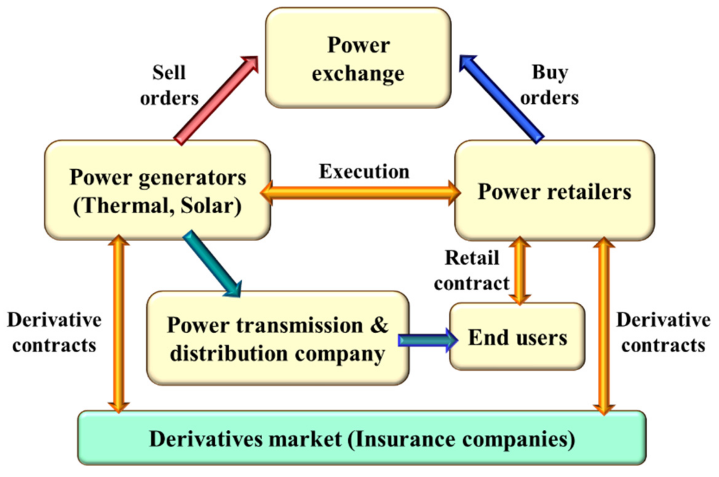
Figure 1 depicts the electricity and derivatives transactions considered in this study. We assume that there is a derivatives market that enables power generators and retailers to execute derivative contracts with arbitrary payoff functions. The power generators and retailers first solve the hedging problems with an appropriate choice of variables, as shown in items 1–3. Then, find a counterparty who agrees with the transaction to execute the derivative contracts. Potential candidates of such counterparties are insurance companies, and we assume that insurance companies can execute the electricity and weather derivative transactions with any payoff functions. Note that, since the net payoffs of derivatives are supposed to be zero on average, the insurance companies can make a profit if a small commission or transaction fee is purchased for each transaction. Furthermore, since the insurance companies can make transactions with power retailers and generators simultaneously, who may cause cashflows in opposite directions, the insurance companies’ risks may be reduced (see Section 5).

Figure 1.
Transaction model of electricity and derivatives.
In the case of the forward contracts in (3), it may be possible to introduce market makers (e.g., insurance companies or financial institutions) who provide fair bid and ask prices and accept sell and buy orders from power generators and retailers. Note that market makers can make a profit from the bid–ask spread, whose sizes are limited by regulations in the market. If the numbers of short and long positions are the same for the same product, the market makers do not have any risks. Therefore, the balance between the long and short positions is important for estimating the market maker’s risk. In this study, we will not analyze such balance risk between long and short positions for forward contracts, but only demonstrate the risk reduction of insurance companies by simultaneously making transactions of derivative contracts with power retailers and generators. A detailed analysis of the balance risk for forward transactions will be left for future work.
Note that, since retailers will typically have already made electricity delivery contracts for any consumed volume over longer durations, the cashflow risk with high volatility in some hours would be a serious concern, as discussed in [9]. In addition, solar power generators may be concerned about a significant drop or surplus in output because of the weather, and so may suffer from unexpected high or low prices as well as volume fluctuation for the power output. Therefore, a selective hedge against the price and volume fluctuation in particular hours would be desirable. Considering the above, we will represent hourly and daily periods using different indexes and define the variables accordingly after this section. In that case, the subscript will be used for a day index whereas will be used for an hour index. For example, the spot price on day at hour will be denoted as in Section 3 and thereafter.
3. Estimation and Test Procedures
In this section, we will explain the statistical estimation models to solve our hedging problems. Since the basic idea is already explained in our previous literature [28,29,33], we will briefly summarize our hedging models.
3.1. Variables Used for Hedging Problems
We will express the variables using the day and hour indexes. Let be the observation data period on a daily basis and be an hour index. Then, the spot price delivering 1 kWh of electricity from hour (to hour ) on day is denoted by Furthermore, the volume is defined , but depending on the situation we may specify the category of the volume using a superscript such as and , respectively, for the total volume of retailers (i.e., consumers’ demand), the total PV generation, and the total thermal generation. In this study, we construct hedging models for each and demonstrate the hedge effects.
For the weather index data , we used hourly temperature and solar radiation data, denoted by and . Note that the choice of weather index data is different for power retailers, solar PV generators, and thermal generators, and is given by , and , respectively. In addition, when weather data are available at multiple points in one region, we compute a local demand weighted average for temperature and an installed capacity of local PV weighted average for radiation, respectively, and create the temperature and radiation indexes.
3.2. Minimum Variance Hedging Using Derivatives
Consider the minimum variance hedging problem with the payoff functions of the derivatives in (2). To find the optimal payoff functions, we apply GAM for each as follows:
where and are smoothing spline functions to be estimated in GAM and is a residual satisfying zero mean condition, .
In (6), contains day of week, long-term, and seasonal trends as
where and are day of week and holiday dummy variables that take if the day of is Monday or otherwise, and so on. denotes a yearly cyclical smoothing spline function and reflects the seasonal trend in , whereas is a smoothing spline function (e.g., a cubic spline function) of the day variable . These functions can be estimated using the day dummy variables. Note that the coefficients and spline functions in (7) are different by hour , but we omit specifying this dependence for brevity. In addition, because the solar power may be independent of the day of the week and holidays, we assume that for solar PV generations.
For each , GAMs can be estimated by minimizing the following penalized residual sum of squares (PRSS):
where is the number of observations for each variable. In (8), the first term is the sum of squares for residuals, and the second term provides the smoothness constraint on spline functions with smoothing parameter vector , where is the number of smoothing spline functions in GAMs, and the larger the , the smoother the th spline function. The smoothing parameter vector needs to be fixed a priori, but an optimal may be searched based on the generalized cross-validation criteria, as shown in [35].
Then, the PRSS is minimized over smoothing spline functions and coefficients given to construct the GAMs.
From (6), we have
Hence, minimizing the sample variance of with smoothing conditions may be considered as PRSS minimization. Note that we can add the constraints and when solving the PRSS so that is satisfied. In this case, we have , and may be considered as the time trend, such as day, seasonal, and long-term contained in . In practice, the deterministic term may be replicated by buying a bound that pays off the same amount of at the settlement period. Consequently, we conclude that the minimum variance hedging problem (1) with (2) can be formulated using GAM (6).
3.3. Minimum Variance Hedging Using Forwards
In the previous subsection, we explained that the optimal payoff functions of electricity and weather derivatives may be found by applying GAM. Here, we show that the minimum variance hedging problem (1) with (3), in which the payoff is defined by time-dependent forward positions, may also be formulated using GAM.
Consider the following GAM with cross variables, and :
where and are smoothing spline functions to be estimated and is a residual satisfying zero mean condition, . The smoothing spline functions, and , are given by a yearly cyclical smoothing spline function like in (7). Note that in the case of the solar PV generators hedging problem, a long-term trend (like ) may be added.
In GAM (10), forward prices, and , are not specified explicitly, but we can show that and may be extracted from by decomposing as
where and are forward prices satisfying , and is an additional term that may be calculated by (11) after and are found. The calculation of and requires solving additional regression problems, but as far as hedge errors are concerned, we do not have to explicitly specify and . Then, we see that minimizing the sample variance of with smoothing conditions may be considered as the minimum variance hedging problem (1) with (3), that is,
3.4. Empirical Test Procedure
As explained in the end of Section 2.1, our empirical test consists of parameter estimation and performance verification based on in-sample and out-of-sample data, respectively. Assume that the entire data period is given by in which the hourly data are also available. Our empirical test procedure is as follows:
- Step 1.
- Given observation data of and , split the data period into and
- Step 2.
- For each hourly period apply GAM (6) (or GAM (10)) to find optimal smooth functions, and ( and ), and calendar trend function, ;
- Step 3.
- For the optimal smooth functions and obtained in Step 2, compute the out-of-sample hedge errors by
- Step 4.
- For the out-of-sample data of , evaluate the out-of-sample hedge performance using the following variance reduction rate (VRR):and the normalized mean absolute error (NMAE),
4. Empirical Hedge Simulations
In this section, we conduct empirical simulations of our hedging problems and demonstrate hedge performance using Japanese electricity market and meteorological data. (In this study, we estimate GAMs using R 4.0.5 (https://www.R-project.org/, accessed on 27 October 2021) and the package mgcv [37] (https://cran.r-project.org/web/packages/mgcv/index.html, accessed on 27 October 2021) to obtain the series of smoothing spline functions, wherein the smoothing parameter is calculated by the generalized cross-validation criterion. All figures are plotted using MATLAB 2021a (MathWorks, Inc., Natick, MA, USA).)
4.1. Data
We use the electricity price, volume, and weather data observed in the Tokyo area, Japan. The data period is chosen from 1 April 2016 (when the Japanese electricity market was fully liberalized) to 31 December 2019, in which we set the first three years (from 1 April 2016 to 31 March 2019) as the in-sample estimation period and the remaining 275 days (from 1 April 2019 to 31 December 2019) was reserved for the out-of-sample performance evaluation.
The following is the list of data used in our analysis:
- Electricity price [Yen/kWh]: JEPX spot price in Tokyo area (JEPX Tokyo area price) delivering 1 kWh of electricity from hours to (downloaded from http://www.jepx.org/market/index.html, accessed on 27 October 2021); since the length of delivery is 30 min for JEPX spot prices, we compute the average of two consecutive prices per hour; for example, we compute the average of 1:00–1:30 p.m. and 1:30–2:00 p.m. delivery prices for the 1:00–2:00 p.m. price;
- Volume [kWh]: Hourly realized demand and supply data in the Tokyo area, including the total demand (), the total solar power generation (, and the total thermal power generation between hours and on day (downloaded from https://www.tepco.co.jp/forecast/html/area_data-j.html, accessed on 27 October 2021);
- Temperature [°C]: We use hourly realized temperature data on day in the Tokyo area (downloaded from https://www.data.jma.go.jp/gmd/risk/obsdl/, accessed on 27 October 2021). A temperature index is constructed using the electricity consumption-based weighted average of nine observation points (we used the yearly local electricity consumption data in Tokyo area as of the end of March 2016, obtained from https://www.tepco.co.jp/corporateinfo/illustrated/business/business-scale-area-j.html, accessed on 27 October 2021);
- Solar radiation [MJ/m2]: We use hourly realized solar radiation data on day in the Tokyo area (downloaded from https://www.data.jma.go.jp/gmd/risk/obsdl/, accessed on 27 October 2021). A solar radiation index is constructed using an installed capacity of local PV weighted average of seven observation points (we used the installation capacity data in Tokyo area as of the end of March 2019 (corresponding to the end of in-sample period), obtained from https://www.fit-portal.go.jp/PublicInfoSummary, accessed on 27 October 2021).
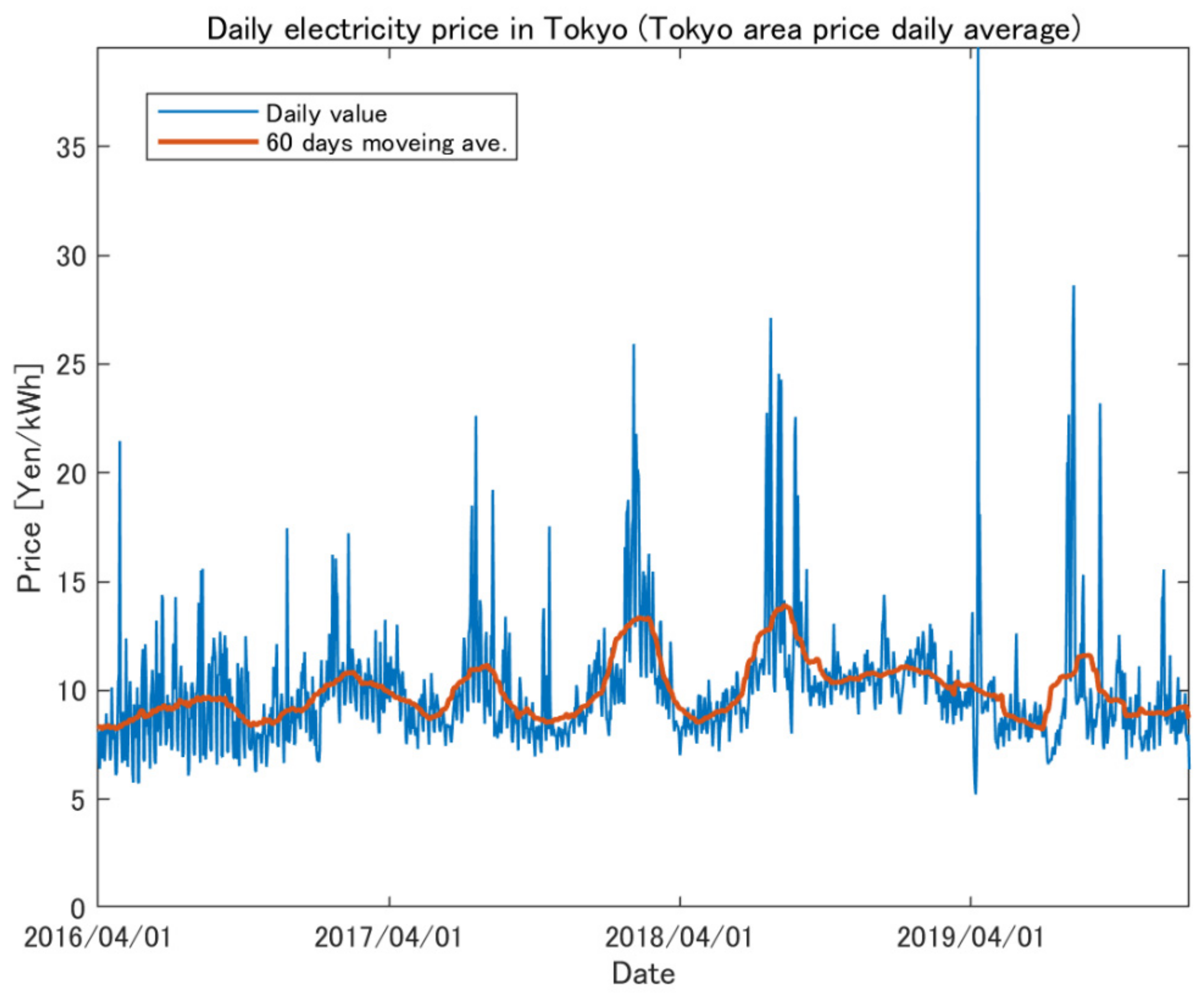
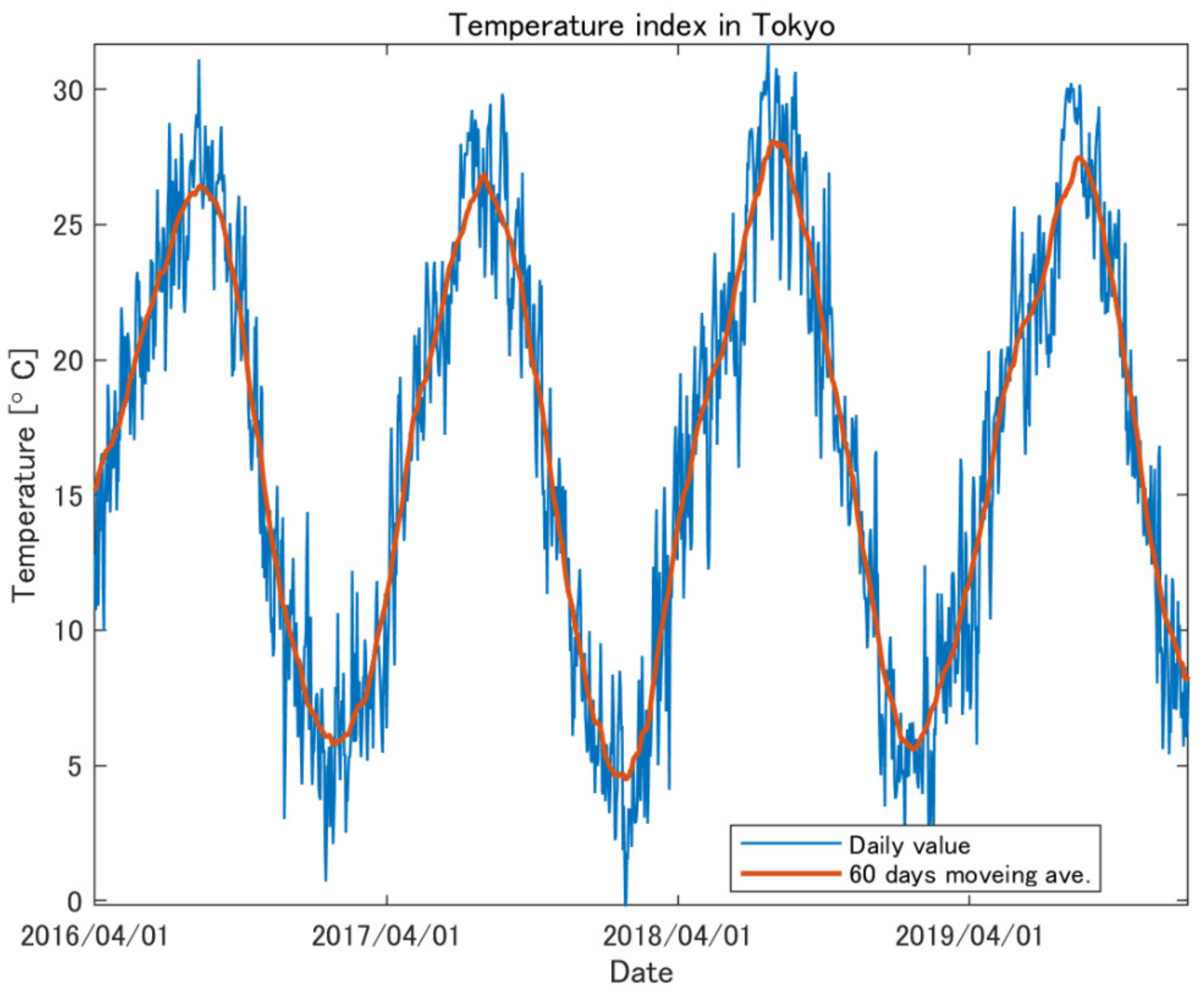
Figure 2 shows the daily electricity price in the entire period, where the blue line is the fluctuation of the daily spot price (i.e., the average of 30 min prices per day) and the red line is the 60 days moving average. Figure 3 provides the volume data of solar PV and thermal generations in total, as well as the total supply (which is the same as the total demand) in the Tokyo area. Figure 4 shows the temperature index in the Tokyo area, where the average temperature for 24 h per day and its 60 days moving average are plotted as the blue and red lines, respectively. Similarly, Figure 5 provides the solar radiation index in the Tokyo area. Note that the temperature and radiation indexes are constructed by taking the weighted averages of several observation points by local electricity consumption and installation capacities of local PV generation in Tokyo, respectively. Furthermore, note that these figures are plotted daily by taking averages, but we construct hedging models based on hourly data, as explained in the previous section.

Figure 2.
Daily average price in Tokyo and its 60 days moving average in the period of 1 April 2016 to 31 December 2019.
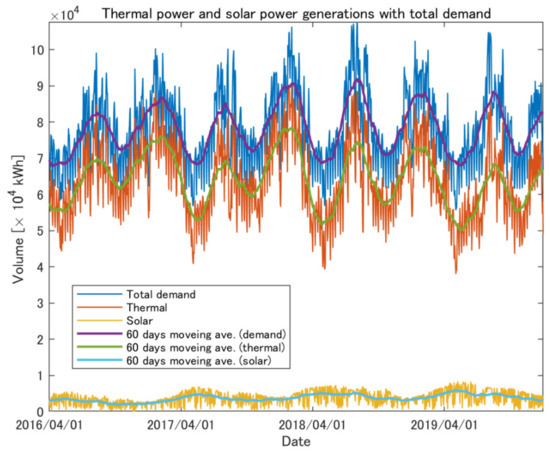
Figure 3.
Daily fluctuations of thermal power and solar power generations, total demand, and their 60 days moving averages in the period of 1 April 2016 to 31 December 2019.

Figure 4.
Daily average of temperature index in Tokyo and its 60 days moving average in the period of 1 April 2016 to 31 December 2019.
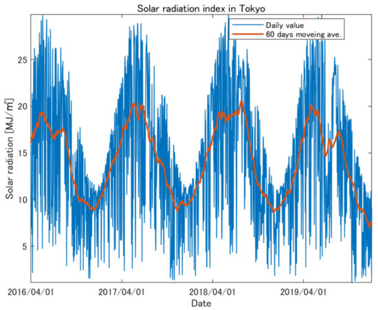
Figure 5.
Daily average of solar radiation index in Tokyo and its 60 days moving average in the period of 1 April 2016 to 31 December 2019.
4.2. Estimation Result for Power Retailers’ Hedges
First, we solved the minimum variance hedging problem for power retailers (or equivalently, the hedging problem of the load retailer) by applying GAM (6) with and . We estimated the optimal spline functions and other required parameters in (6) based on the in-sample data. Then, we computed the out-of-sample hedge errors based on Equation (13) to evaluate the hedge performance in terms of VRR and NMAE in (14) and (15), respectively.
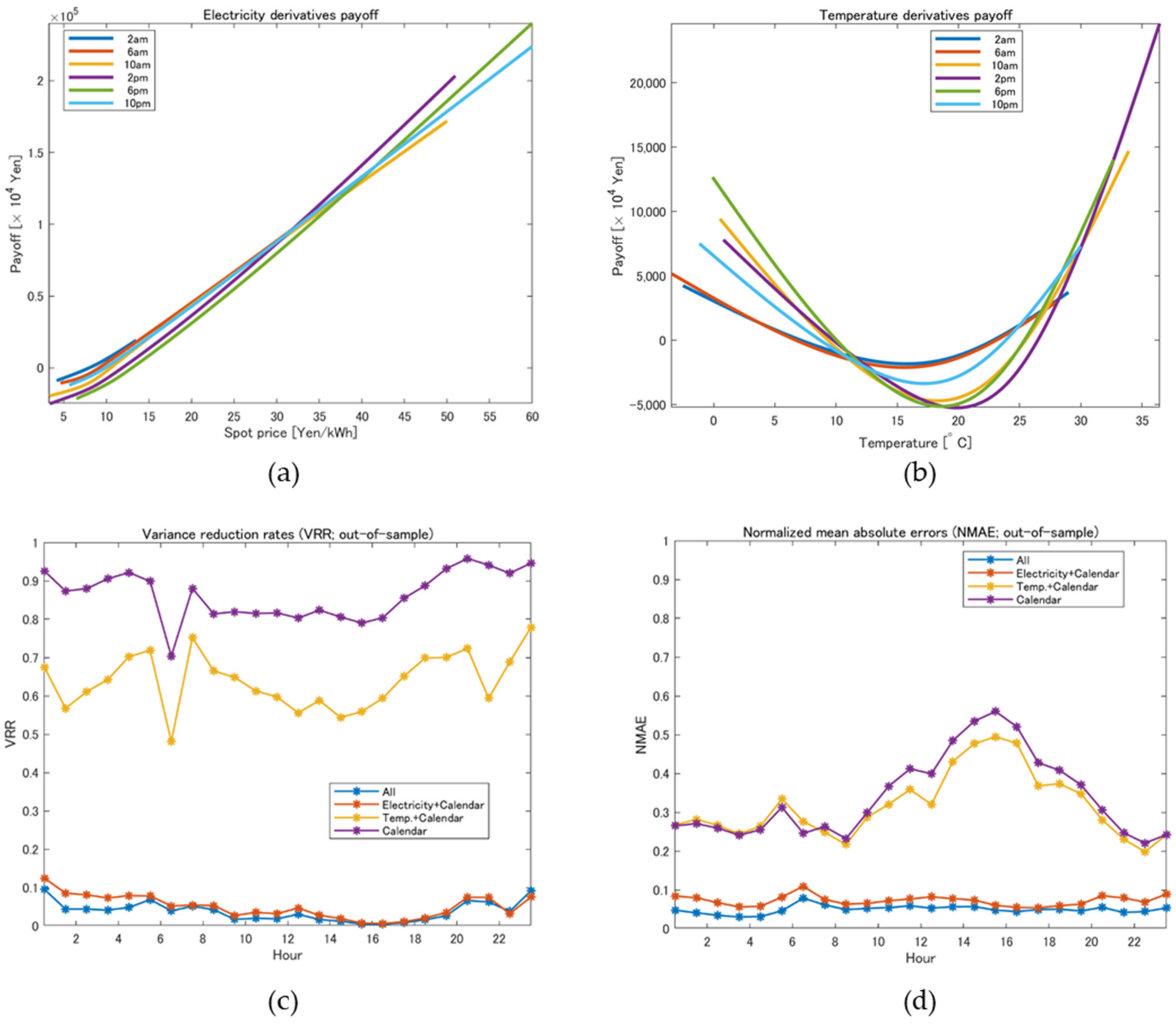
Panels (a) and (b) of Figure 6 represent the payoff functions estimated by applying GAM (6), where the payoff functions of electricity derivatives for are plotted in panel (a) among 24 estimated functions and those of temperature derivatives, , are shown in panel (b). These payoff functions satisfy and given the parameter estimation period and may provide negative values of the payoffs. We see that the payoff functions for electricity derivatives increase monotonically, whereas those of temperature derivatives increase with a larger temperature and a smaller temperature for both sides. The latter is interpreted as the effects of temperature on electricity demand. For example, the payoff function at 2 p.m. increases rapidly when the temperature is higher than 25 °C, reflecting the electricity consumption in summer for the usage of air conditioners. In addition, in the morning and the evening (e.g., 10 a.m. and 6 p.m.), the payoff functions increase rapidly when the temperature is below 10 °C mainly from the electricity consumption in winter.
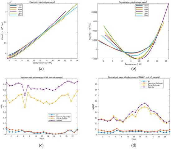
Figure 6.
Results of minimum variance hedging with derivatives for electricity retailers’ cash flows, , based on empirical data: (a) optimal payoff functions of electricity derivatives; (b) optimal payoff functions of temperature derivatives; (c) out-of-sample VRR for each hour; (d) out-of-sample NMAE for each hour.
Panels (c) and (d) represent the out-of-sample hedge performance of our methodology, which provide VRRs and NMAEs computed by Equations (14) and (15), respectively. Note that both blue lines at the bottom of the figures are those obtained by using GAM (6) for different values of , whereas other lines are obtained by applying GAMs with (electricity derivative) and only, (temperature derivative) and only, and only, respectively. These lines are plotted as red, yellow, and purple lines, respectively, in panels (c) and (d). Comparing the purple and red lines, we see that the hedge performance is improved significantly by incorporating electricity derivatives. Then, the VRRs and NMAEs are further improved by adding temperature derivatives.
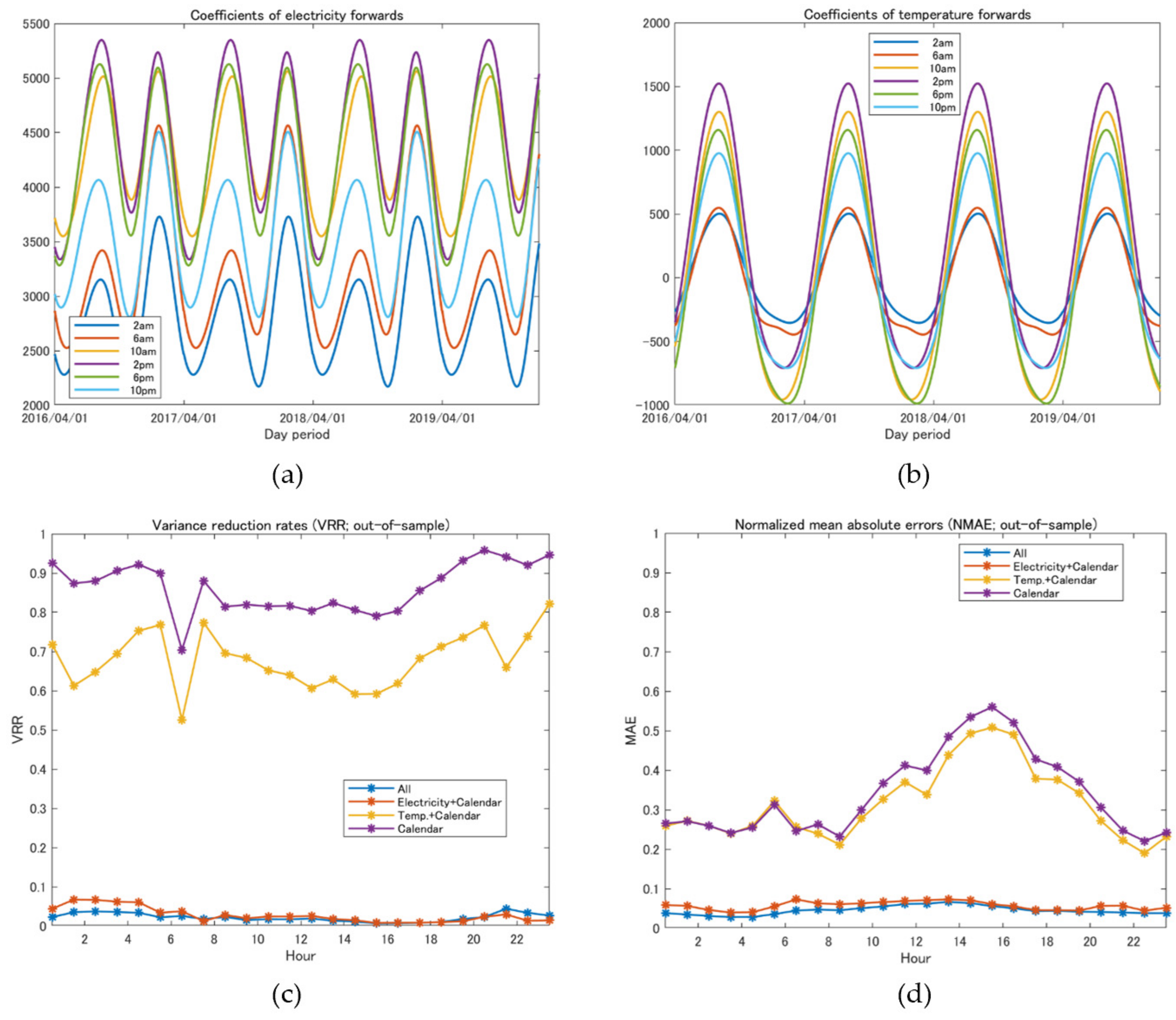
Furthermore, we solved the minimum variance hedging problem (1) with (3) to find the optimal coefficients of forward contracts, and , by applying GAM (10) based on in-sample data. Panels (a) and (b) of Figure 7 provide the estimation results, where the estimated values of and are plotted, providing the coefficients of electricity forwards and temperature forwards, respectively. The dates of the in-sample and out-of-sample periods are assigned on the horizontal axes instead of the day and cyclical dummy variables used for the estimation of GAM (10). Since we assumed that the in-sample data period was until 31 March 2019, the estimated functions after 1 April 2019 provide the predicted values of the coefficients. We see that the coefficients of electricity forwards have two peaks in a year, which reflect the demand peaks in summer and winter.
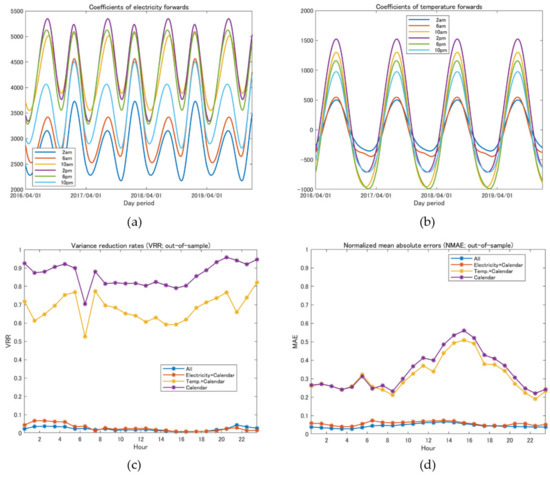
Figure 7.
Results of minimum variance hedging with forwards for electricity retailers’ cash flows, , based on empirical data: (a) coefficients of electricity forwards; (b) coefficients of temperature forwards; (c) out-of-sample VRR for each hour; (d) out-of-sample NMAE for each hour.
The coefficients of temperatures reflect the effect of temperature on demand. For example, in summer the demand has a positive correlation with temperature, whereas in winter the correlation becomes negative so that the demand increases as the temperature decreases. Panels (c) and (d) show out-of-sample VRRs and NMAEs. Like panels (c) and (d) of Figure 6, we see that the hedge performance is improved significantly by incorporating electricity forwards, which is further improved by adding temperature forwards.
4.3. Estimation Results for Solar PV Generators’ Hedges
Next, we demonstrate our empirical results for hedging problems with solar PV generations. To the end, we applied GAMs (6) and (10) to solve the minimum variance hedging problems with and , as with the previous subsection, but the hour index is restricted to the range of and the solar PV generations from 8 a.m. to 4 p.m. are considered. We estimated the optimal spline functions and other required parameters in (6) and (10) based on in-sample data and computed out-of-sample hedge errors.
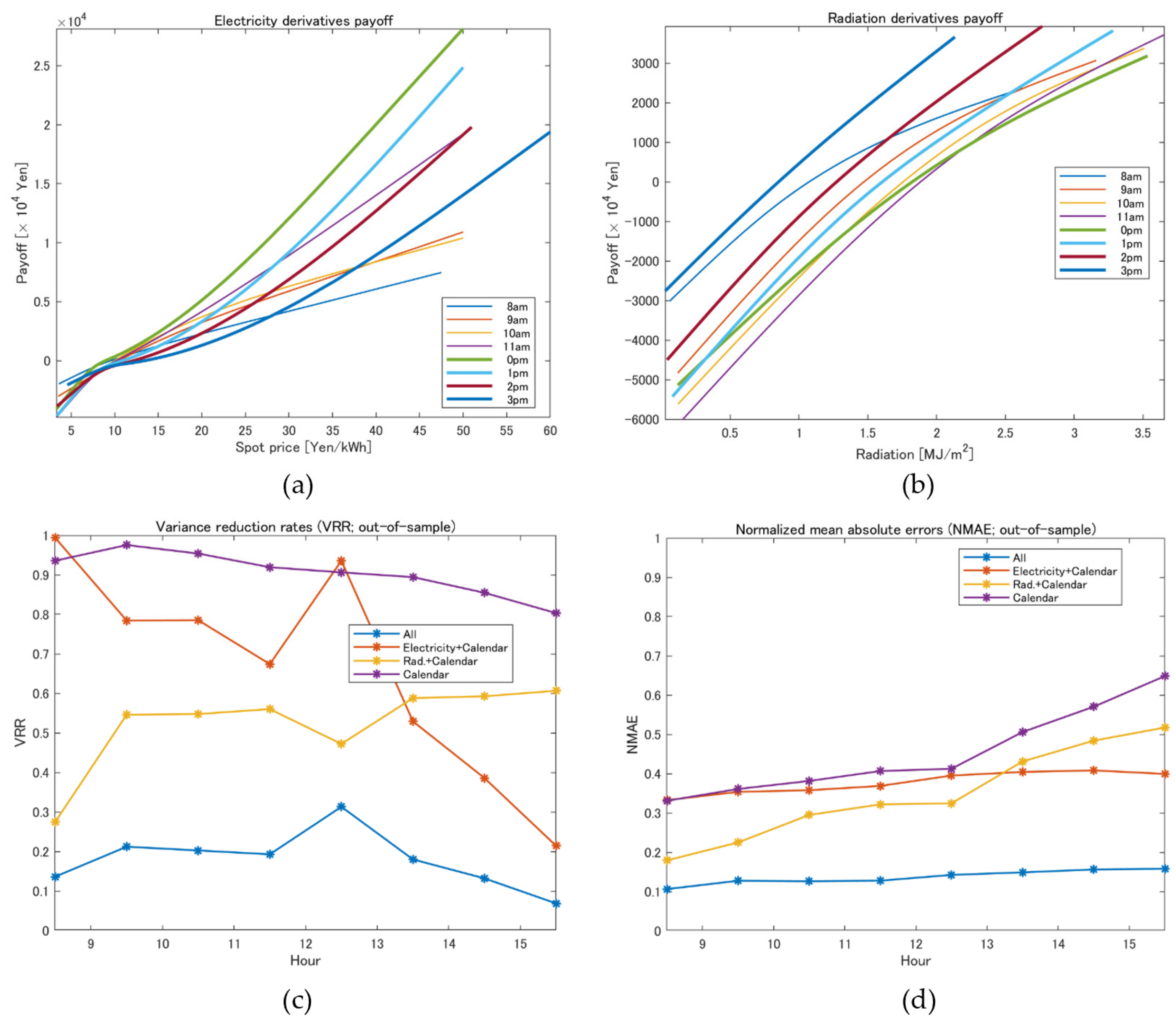
Figure 8 and Figure 9 present the empirical results. Panels (a) and (b) in Figure 8 represent the payoff functions estimated by applying GAM (6), where the payoff functions of electricity derivatives and radiation derivatives, and , for are plotted, respectively. These payoff functions satisfy and given the parameter estimation period and may provide negative values of the payoffs. We see that both the payoff functions for electricity and radiation derivatives increase monotonically, incorporating the effects of electricity price and solar PV generation on the cashflow. Panels (c) and (d) in Figure 8 provide out-of-sample VRRs and NMAEs, respectively, which were computed by applying Equations (14) and (15) based on out-of-sample data. Similar to panels (c) and (d) in Figure 6, the blue lines denote VRRs and NMAEs obtained using all the terms in GAM (6), whereas other lines were obtained with (electricity derivative), only; (radiation derivative), only; and only. Although both VRRs and NMAEs were not improved significantly by electricity derivatives compared to Figure 6, we see that the combinations of electricity and radiation derivatives largely improved VRRs and NMAEs. Thus, we conclude that radiation derivatives are effective for hedging problems.

Figure 8.
Results of minimum variance hedging with derivatives for solar PV generators’ cash flows, , based on empirical data: (a) optimal payoff functions of electricity derivatives; (b) optimal payoff functions of solar radiation derivatives; (c) out-of-sample VRR for each hour; (d) out-of-sample NMAE for each hour.
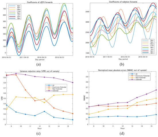
Figure 9.
Results of minimum variance hedging with forwards for solar PV generators’ cash flows, , based on empirical data: (a) coefficients of electricity forwards; (b) coefficients of solar radiation forwards; (c) out-of-sample VRR for each hour; (d) out-of-sample NMAE for each hour.
Panels (a) and (b) of Figure 9 provide the estimated values of and corresponding to the coefficients of electricity forwards and radiation forwards, respectively. Like panels (a) and (b) of Figure 7, the day dummy variables are replaced by the dates of the in-sample and out-of-sample periods. In these figures, we see that both coefficients have increasing trends, which incorporate the increase in total PV generation in the Tokyo area. Furthermore, the periodicity of these coefficients reflects the seasonality of solar radiation in a year. Panels (c) and (d) show out-of-sample VRRs and NMAEs, like Figure 8. From these figures, we see that the hedge performance was improved significantly by incorporating both electricity and radiation forwards.
4.4. Estimation Results for Thermal Generators’ Hedges
Finally, we present our empirical simulation results for hedging problems with thermal generations. To this end, we applied the following GAMs with and , respectively, for constructing derivatives and forwards:
where and in (16) are smoothing spline functions, and in (17) are cyclic spline functions, and is a residual term satisfying . Note that we used a separate notation for a function of in (16) to emphasize that and are individual single variate functions. We estimated optimal spline functions and other required parameters in (16) and (17) based on in-sample data and computed out-of-sample hedge errors like those in the previous subsections.
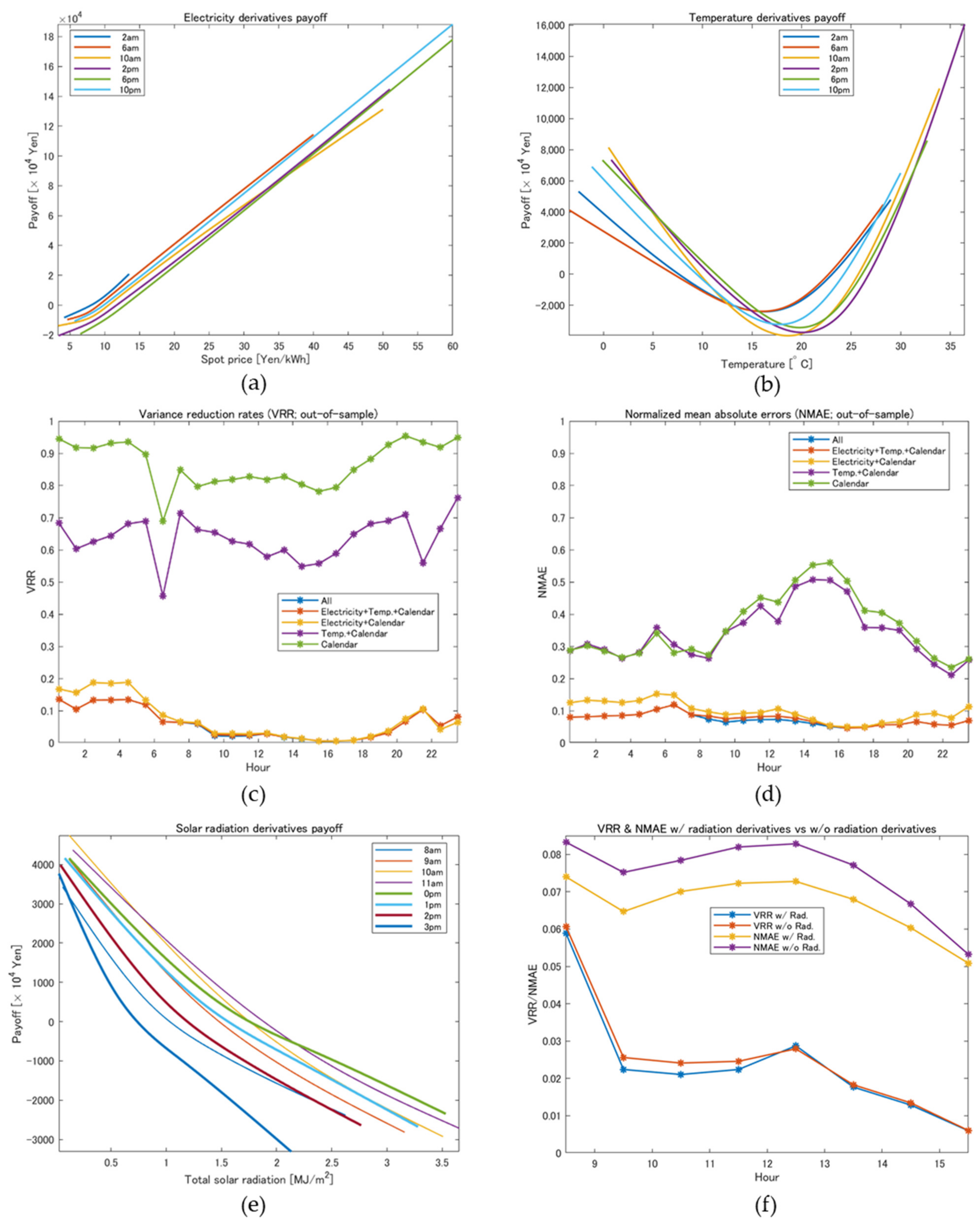
Panels (a) and (b) in Figure 10 represent the estimated payoff functions, and , for electricity derivatives and temperature derivatives, respectively. Like other payoff functions, these functions satisfy and given the parameter estimation period and may provide negative payoffs. We see that the shapes of both payoff functions are like those in Figure 8 but have different scales in the y-axis. This is because the volume covered by thermal generation was approximately 80% on average with respect to the total demand for the period of our analysis. Panels (c) and (d) in Figure 10 provide out-of-sample VRRs and NMAEs, respectively, which were computed by applying Equations (14) and (15) based on out-of-sample data. In this test, radiation derivatives were included for only, and we estimated the payoff functions of radiation derivatives, as shown in panel (e). In these figures, note that VRRs and NMAEs, including radiation derivatives, are plotted using blue lines, although they are almost hidden by the red lines corresponding to VRRs and NMAEs without radiation derivatives. To emphasize the difference between them, we further plotted VRRs and NMAEs with and without radiation derivatives, as shown in panel (f). Then, we can observe that the radiation derivatives contribute to the improvement of out-of-sample hedge performance.
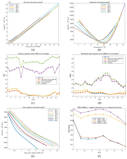
Figure 10.
Results of minimum variance hedging with derivatives for thermal generators’ cash flows, : (a) optimal payoff functions of electricity derivatives; (b) optimal payoff functions of temperature derivatives; (c) out-of-sample VRR for each hour; (d) out-of-sample NMAE for each hour; (e) optimal payoff functions of radiation derivatives; (f) out-of-sample VRR & NMAE with or without radiation derivatives for each hour.
Panels (a) and (b) of Figure 11 provide the estimated values for the coefficients of electricity forwards and temperature forwards, respectively. In the hedging problems with forwards, radiation terms were included for and their coefficients were computed, as shown in panel (e). Like the previous figures, the day dummy variables were replaced by the dates of in-sample and out-of-sample periods. Furthermore, panels (c) and (d) show out-of-sample VRRs and NMAEs. In these figures, the blue lines provide VRRs and NMEs with radiation derivatives; however, they are almost completely hidden. Then, we further investigated VRRs and NMAEs with and without radiation forwards, as shown in panel (f). However, it turned out that the contribution of radiation forwards to the improvement of hedge effect was weak and unstable compared to the case of radiation derivatives, at least in the out-of-sample simulations.
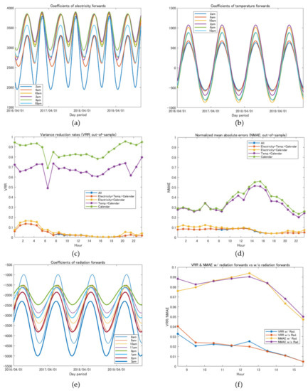
Figure 11.
Results of minimum variance hedging with forwards for thermal generators’ cash flows, : (a) optimal coefficients functions of electricity forwards; (b) optimal coefficients of temperature forwards; (c) out-of-sample VRR for each hour; (d) out-of-sample NMAE for each hour; (e) optimal coefficients of radiation forwards; (f) out-of-sample VRR & NMAE with or without radiation forwards for each hour.
To compare the cross-sectional hedge performance, we computed the averages of hourly VRRs and NMAEs in the out-of-sample period, corresponding to the averages of “All” (the blue lines) in panels (c) and (d) of Figure 6, Figure 7, Figure 8, Figure 9, Figure 10 and Figure 11, respectively. Table 1 provides the averages of VRRs and NMAEs of minimum variance hedging problems for retailers, solar PV generators, and thermal generators, where the averages are taken for in the case of solar PV generators. If compared between minimum variance hedging problems using derivatives and those using forwards for the same electricity utility players (i.e., retailers, solar PV generators, or thermal generators), we see that retailers and thermal generators achieve both better VRRs and NMAEs using forwards, as emphasized by bold letters in Table 1. On the other hand, in the case of solar PV generators, minimum variance hedging using derivatives provides a better hedge performance.

Table 1.
Averages of hourly VRRs and NMAEs in the out-of-sample simulations.
5. Reduction of Risks for Insurance Companies
In this study, we have assumed that the counter parties for derivative contracts are insurance companies (see Figure 1). Then, as explained in Section 2, the risks of insurance companies can be averaged out by executing derivatives or forward contracts with players in different positions, such as power retailers and generators. In this section, we illustrate that the risks of insurance companies can be reduced by executing derivative contracts with such players simultaneously.
5.1. Basic Idea
Assume that there is a derivative contract in the market offered by an insurance company whose payoff at is denoted by and satisfies . Then, the insurance company’s expected cashflow from the derivative is given by , and the insurance company can make a positive profit by receiving a commission from a buyer if the risk of cashflow fluctuation is small. However, there is a possibility that large cashflow fluctuations lead to a significant loss to insurance companies, and so the insurance company needs to evaluate the risk a priori; one measure of such risk is given by its variance.
We further assume that there exists another derivative contract offered by another insurance company, whose payoff at time is and satisfies . Then, the aggregate risk in the market from and may be given by the sum of variances, . Instead of considering aggregate risk, one may introduce the risk of aggregate cashflow, , defined by This may be a situation of evaluating the risk of an insurance company that is willing to offer both derivatives with payoffs, and , and the following quantity provides a relative effectiveness of such position compared to the aggregate risk in the market:
If and are independent in (18), we see that and that the quantity in (18) equals . On the other hand, if and are negatively correlated, then holds and the quantity in (18) becomes less than 1, which leads to a reduction in variance by combining two cashflows. In this sense, the quantity in (18) measures the variance reduction effect of the two cashflows for the insurance company.
In general, assuming that are cashflows from derivative contracts executed with power retailers and generators, the insurance company’s VRR may be defined as follows:
Furthermore, we define the insurance company’s NMAE as
Note that the sum of cashflows in (20) is not an error, but we use the same terminology as the previous definitions to avoid a redundant definition. Although we can introduce insurance companies’ VRR and NMAE for cashflows from forward contracts as well, here we focus on the cashflows from derivative contracts only; that is, we consider cashflows of derivatives obtained by solving minimum variance hedging problems for power retailers and generators.
5.2. Evaluation of Insurance Company’s VRRs and NMAEs Using Empirical Data
Now, we evaluate insurance companies’ VRRs and NMAEs using empirical data. Let , , and be the payoff functions of the electricity derivatives obtained by applying GAM (6) with and for power retailers, GAM (6) with and for solar PV generators, and and for thermal generators, where these payoff functions are estimated using in-sample data, as shown in panel (a) of Figure 6, Figure 8, and Figure 10, respectively.
Assume that all transactions of electricity derivatives in hedging problems are executed with the same insurance company. Since the direction of cashflow for exchanging the electricity delivery contract through power exchange is opposite between power retailers and generators, the insurance company is supposed to pay to retailers and receive and from power generators. Therefore, the aggregate cashflow (i.e., cash-out from the insurance company) is given as
Panels (a) and (b) in Figure 12 show the cashflows from the payoffs of electricity derivatives, where the blue line is the payoff of derivatives that the retailer receives and the red line is the sum of payoffs for generators (i.e., the solar power generator and the thermal generator). Panel (a) represents cashflows corresponding to the electricity delivery of 10–11 a.m. and panel (b) cashflows for 2–3 p.m. In these figures, the x-axis denotes the dates of the in-sample and out-of-sample periods, in which the in-sample period is until 31 March 2019. The yellow lines provide the aggregate cashflows of (21).
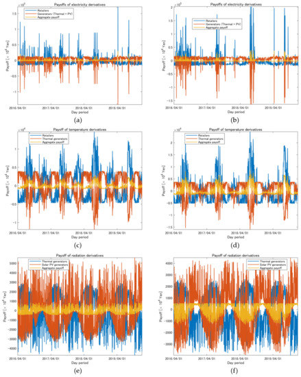
Figure 12.
Cash flows (CFs) from derivatives payoffs: (a) payoff of retailers, the sum of payoffs for thermal generators and solar PV generators, and their aggregate payoff from electricity derivatives for 10–11 a.m.; (b) payoff of retailers, the sum of payoffs for thermal generators and solar PV generators, and their aggregate payoff from electricity derivatives for 2–3 p.m.; (c) payoffs of retailers and thermal generators and their aggregate payoff from temperature derivatives for 10–11 a.m.; (d) payoffs of retailers and thermal generators and their aggregate payoff from temperature derivatives for 2–3 p.m.; (e) payoffs of thermal generators and solar PV generators and their aggregate payoff from radiation derivatives for 10–11 a.m.; (f) payoffs of thermal generators and solar PV generators and their aggregate payoff from radiation derivatives for 2–3 p.m.
Similarly, panels (c) and (d) show the cashflows from payoffs of temperature derivatives, and panels (e) and (f) those of radiation derivatives. In these cases, the aggregate cashflows are given by
for temperature derivatives, and
for radiation derivatives, where the optimal payoff functions in (22) and (23) are obtained by applying GAM (6) with appropriate variables. The superscripts of these functions denote the problems we have solved. For example, is obtained by solving the minimum variance hedging problem for retailers and provides the retailer’s payoff of temperature derivatives. The minus signs in front of payoff functions for power generators indicate that the direction of cashflows defined by payoff functions is opposite from that for retailers. For example, the payoff that the thermal generator receives is defined by .
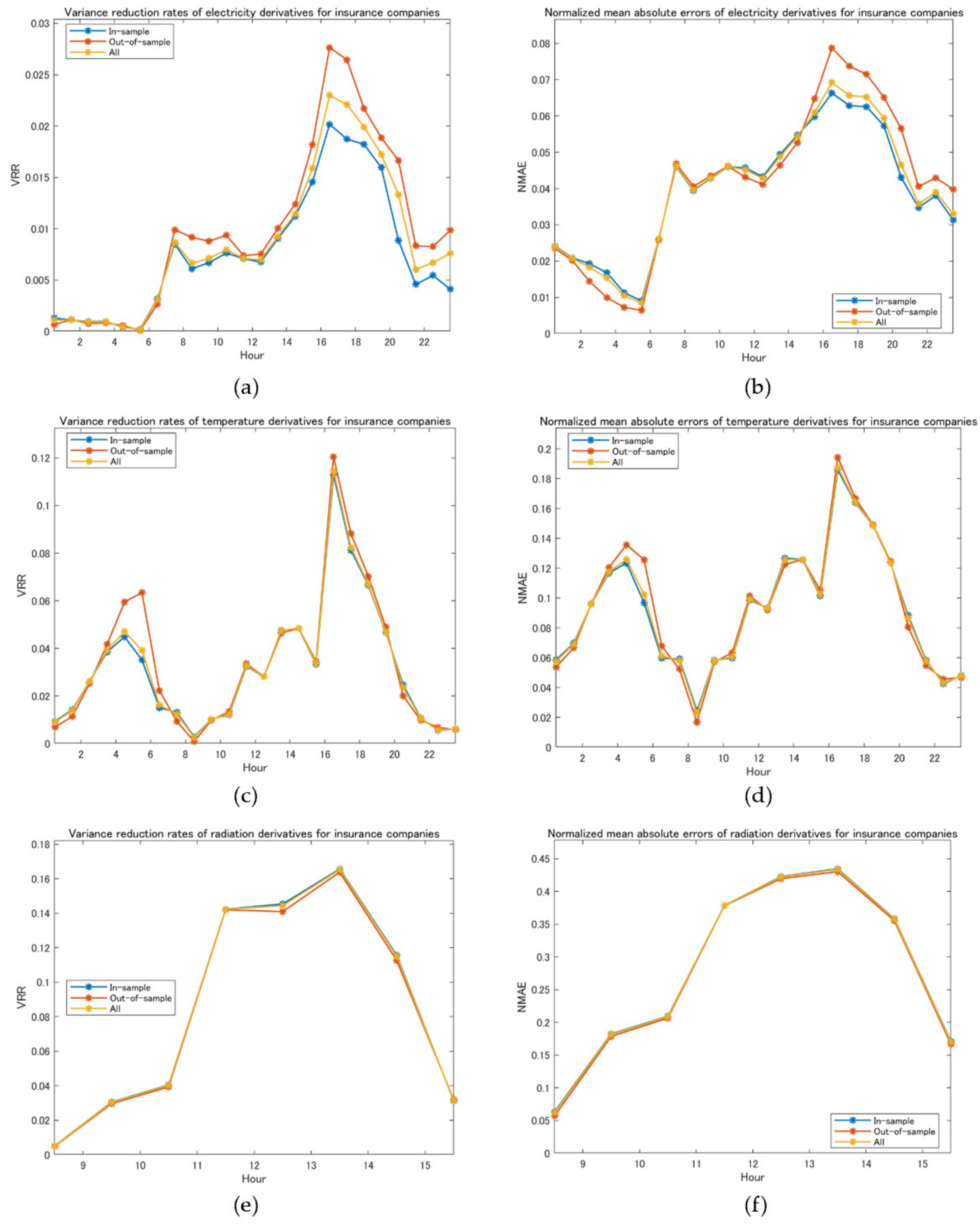
Panels (a) and (b) of Figure 13 provide insurance companies’ VRRs and NMAEs of electricity derivatives, respectively, for each , where the blue lines denote those obtained by using in-sample data, the red lines denote those obtained using out-of-sample data, and the yellow lines indicate the entire period data. Since the aggregate cashflow is given by (21), the insurance company’s VRRs and NMAEs are computed by replacing , and in (19) and (20), respectively. From these figures, we see that both VRRs and NMAEs are small in the case of electricity derivative transactions, and the variance is reduced significantly by combining cashflows from derivatives executed with retailers and generators.
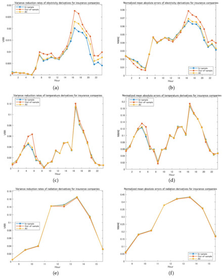
Figure 13.
Variance reduction rates (VRRs) and normalized mean absolute errors (NMAEs) for insurance companies’ cash flows (CFs): (a) VRRs for CFs of electricity derivatives’ payoffs; (b) NMAEs for CFs of electricity derivatives’ payoffs; (c) VRRs for CFs of temperature derivatives’ payoffs; (d) NMAEs for CFs of temperature derivatives’ payoffs; (e) VRRs for CFs of radiation derivatives’ payoffs; (f) NMAEs for CFs of radiation derivatives’ payoffs.
Panels (c)–(f) provide insurance companies’ VRRs and NMAEs of temperature and radiation derivatives, respectively, like panels (a) and (b) of electricity derivatives. In the case of temperature derivatives, the aggregate cashflow of (22) consists of and , whereas that of (23) consists of and in the case of radiation derivatives, respectively. Then, the VRRs and NMAEs are computed based on (19) and (20). From these figures, we see that the risk reduction effect is reasonably significant, although it is not as large as that of electricity derivatives.
6. Discussion
In this study, we have systematically organized the theoretical aspects of our previous studies in [33,34] and developed a unified approach using derivatives and forwards on the spot electricity price and weather data. We aim not only to clarify the applicability of our proposed methods, but also to provide a new and useful perspective on hedging schemes involving various electricity utilities, such as power retailers, solar PV generators, and thermal generators. In our empirical analysis, we have measured the hedging effects on their cashflow management using electricity and weather derivatives as well as forward contracts. The key findings of our analysis are summarized below.
- For the hedging problems using derivatives for the power retailers and the thermal generators, the payoff functions of the electricity derivatives increase monotonically with the underlying electricity price, but a nonlinear dependence is observed when the electricity price is low during the day. This seems to reflect the relationship between the PV generation and electricity prices. In general, the electricity price increases with demand, but in the daytime solar radiation tends to increase, resulting in pushing the electricity price in the lower direction;
- The coefficients of the electricity forwards for power retailers’ and thermal generators’ hedges have two peaks in a year, which correspond to the demand increases in summer and winter. On the other hand, the coefficients of temperature forwards incorporate the correlation between the temperature and the demand. That is, the demand increases with a higher temperature and decreases with a lower temperature in summer, whereas in winter it increases with a lower temperature;
- Both derivatives and forwards are generally effective for reducing the cashflow fluctuations, but in the cases of power retailers’ and thermal generators’ hedging problems the out-of-sample VRRs and NMAEs were better for hedging problems using forwards. This may be explained by the fact that both cashflows for the power retailers and the thermal generators are largely dependent on the electricity demand, which may be better explained using the cyclic trend for the forwards than the spline functions for derivatives;
- On the other hand, in the case of the solar PV generators’ hedging problem, the hedge errors were smaller for derivatives in terms of the VRRs and NMAEs. The reason for this difference is that it seems that the radiation derivatives are more effective for reducing the cashflow fluctuations for the solar PV generations. The same phenomenon was observed in the hedging problem for the thermal generators, where the radiation derivatives are more effective for reducing the risk of cashflow fluctuations based on out-of-sample VRRs and NMAEs.
In our analysis, we have assumed that there exist counter parties of derivative and forward transactions, such as insurance companies, and that the electricity utility players can execute electricity and weather derivative transactions with any payoff functions. Such insurance companies can profit if a commission is purchased for every transaction. Moreover, as explained in Section 2 and Section 5, their risks may be averaged out by executing derivative contracts with power retailers and generators simultaneously. This is because their cash flow directions may be different or opposite for the electricity purchase and the payoffs of derivatives may be canceled out. We have illustrated insurance company risk reduction using empirical simulations and obtained the following:
- 5.
- The fluctuations in the aggregate cashflow of the electricity derivative’s payoffs from the hedging problems for power retailers, solar PV generators, and thermal generators were reduced significantly compared to the sum of independent cashflow fluctuations. This indicates that the insurance company can take and cancel out the risk in electricity purchase by combining appropriate positions;
- 6.
- For temperature and radiation derivatives, the risk reduction effect for insurance companies is not as significant as in the case of electricity derivatives; however, their risks were reasonably reduced. Moreover, weather derivatives are useful products for insurance companies compared to other financial instruments because weather indexes are not affected by human activities, at least in a short period. Therefore, fair prices may be set using their mean values, and the risk of cashflow fluctuation may be averaged out if the transaction period is sufficiently long.
Although we have incorporated the seasonal trend (i.e., the cyclic trend) in the coefficients of forwards in our analysis, we should be able to apply the result of [34] for derivatives with cyclic trends using tensor product spline functions. Then, the hedging effect could be further enhanced by designing derivatives with nonlinear payoffs that change gradually by date. However, it is necessary to consider the tradeoff of different advantages between derivatives and forwards in this regard. That is, while forwards have a payoff function that depends only on the underlying asset (i.e., the hedger optimizes the contract volume), derivatives have a payoff function that depends on the hedger’s profit function (i.e., the hedger optimizes the payoff function itself). This means that the forward market may allow liquid transactions among multiple players, while derivatives are subject to bilateral contracts between the risk taker (insurance company) and the hedger. Thus, whether to use derivatives to improve the hedging effectiveness or to use forwards for the liquid transactions is an issue to be considered based on not only the results of the empirical analysis but also the actual market environment and practical needs.
In addition, as a first step to verify the effectiveness of an efficient market-wide hedging scheme, this study conducted an empirical analysis targeting the Tokyo area, where a certain percentage of solar power generation exists, and the necessary public data is sufficiently available. However, further improvements in the design of derivative products, such as increasing the number of observation points to be taken into account in the creation of the weather index, may be necessary when targeting areas with relatively low population density. Moreover, if the introduction of solar power continues to increase, the effectiveness of solar radiation derivatives for hedging solar volume risk will become increasingly effective, and there is a possibility that this method can be applied more widely. The expansion of such application areas and empirical analysis regarding the verification of the versatility of the method will be a future task.
Furthermore, as described at the end of Section 2, it would be interesting to introduce market makers (e.g., insurance companies or financial institutions) who provide fair bid and ask prices and accept sell and buy orders from power generators and retailers in the forward market. If the numbers of short and long positions are the same for the same product, the market makers do not have any risks. Therefore, the balance between the long and short positions is important for estimating the market maker’s risk. Moreover, the inefficiencies of the market that can be assumed in practice, and the bid–ask spreads (or the premiums demanded by the insurers) that they bring about, may be an additional issue to be further investigated. These will be left for future study.
Author Contributions
Conceptualization, Y.Y. and T.M.; methodology, Y.Y. and T.M.; software, Y.Y.; validation, Y.Y.; formal analysis, Y.Y.; investigation, Y.Y. and T.M.; resources, Y.Y.; data curation, Y.Y.; writing—original draft preparation, Y.Y.; writing—review and editing, Y.Y. and T.M.; visualization, Y.Y.; supervision, Y.Y.; project administration, Y.Y.; funding acquisition, Y.Y. and T.M.; All authors have read and agreed to the published version of the manuscript.
Funding
This work was funded by a Grant-in-Aid for Scientific Research (A) 20H00285, Grant-in-Aid for Challenging Research (Exploratory) 19K22024, and Grant-in-Aid for Young Scientists 21K14374 from the Japan Society for the Promotion of Science (JSPS).
Institutional Review Board Statement
Not applicable.
Informed Consent Statement
Not applicable.
Data Availability Statement
Publicly available datasets were analyzed in this study. This data can be found here: http://www.jepx.org/market/index.html (accessed on 27 October 2021); https://www.data.jma.go.jp/gmd/risk/obsdl/ (accessed on 27 October 2021); https://www.tepco.co.jp/forecast/html/area_data-j.html (accessed on 27 October 2021).
Conflicts of Interest
The authors declare no conflict of interest.
References
- Eydeland, A.; Wolyniec, K. Energy and Power Risk Management: New Developments in Modeling, Pricing and Hedging; John Wiley & Sons: New York, NY, USA, 2003. [Google Scholar]
- Clewlow, L.; Strickland, C. Energy Derivative; Lacima Group: Sydney, Australia, 2000; ISBN 0953889602. [Google Scholar]
- Di Masi, G.B.; Kabanov, Y.M.; Runggaldier, W.J. Mean-variance hedging of options on stocks with Markov volatility. Theory Probab. Its Appl. 1994, 39, 173–181. [Google Scholar] [CrossRef]
- Guo, X. Information and option pricing. Quant. Financ. 2001, 1, 38–44. [Google Scholar] [CrossRef]
- Duan, J.C.; Popova, I.; Ritchken, P. Option pricing under regime switching. Quant. Financ. 2002, 2, 116–132. [Google Scholar] [CrossRef] [Green Version]
- Buffington, J.; Elliott, R.J. American options with regime switching. Int. J. Theor. Appl. Financ. 2002, 5, 497–514. [Google Scholar] [CrossRef]
- Oum, Y.; Oren, S.; Deng, S. Hedging Quantity Risk with Standard Power Options in a Competitive Wholesale Electricity Market. Nav. Res. Logist. 2006, 53, 697–712. [Google Scholar] [CrossRef]
- Hinderks, W.J.; Wagner, A. Pricing German Energiewende products: Intraday cap/floor futures. Energy Econ. 2019, 81, 287–296. [Google Scholar] [CrossRef]
- Matsumoto, T.; Bunn, D.W.; Yamada, Y. Pricing electricity day-ahead cap futures with multifactor skew-t densities. Quant. Financ. 2021, in press. [Google Scholar] [CrossRef]
- Berhane, T.; Shibabaw, A.; Awgichew, G.; Walelgn, A. Pricing of weather derivatives based on temperature by obtaining market risk factor from historical data. Model. Earth Syst. Environ. 2020, 7, 871–884. [Google Scholar] [CrossRef]
- Göncü, A. Pricing temperature-based weather derivatives in China. J. Risk Financ. 2011, 13, 32–44. [Google Scholar] [CrossRef]
- Groll, A.; Cabrera, B.L.; Meyer-Brandis, T. A consistent two-factor model for pricing temperature derivatives. Energy Econ. 2016, 55, 112–126. [Google Scholar] [CrossRef] [Green Version]
- Hell, P.; Meyer-Brandis, T.; Rheinländer, T. Consistent factor models for temperature markets. Int. J. Theor. Appl. Financ. 2012, 15, 1250027. [Google Scholar] [CrossRef]
- Meissner, G.; Burke, J. Can we use the Black-Scholes-Merton model to value temperature options? Int. J. Financ. Mark. Deriv. 2011, 2, 298. [Google Scholar] [CrossRef]
- Lee, Y.; Oren, S.S. An equilibrium pricing model for weather derivatives in a multi-commodity setting. Energy Econ. 2009, 31, 702–713. [Google Scholar] [CrossRef] [Green Version]
- Lee, Y.; Oren, S.S. A multi-period equilibrium pricing model of weather derivatives. Energy Syst. 2010, 1, 3–30. [Google Scholar] [CrossRef] [Green Version]
- Davis, M. Pricing weather derivatives by marginal value. Quant. Financ. 2001, 1, 305–308. [Google Scholar] [CrossRef]
- Platen, E.; West, J. A Fair Pricing Approach to Weather Derivatives. Asia-Pac. Financ. Mark. 2004, 11, 23–53. [Google Scholar] [CrossRef]
- Brockett, P.L.; Wang, M.; Yang, C.; Zou, H. Portfolio Effects and Valuation of Weather Derivatives. Financ. Rev. 2006, 41, 55–76. [Google Scholar] [CrossRef]
- Kanamura, T.; Ohashi, K. Pricing summer day options by good-deal bounds. Energy Econ. 2009, 31, 289–297. [Google Scholar] [CrossRef]
- Benth, F.E.; Di Persio, L.; Lavagnini, S. Stochastic Modeling of Wind Derivatives in Energy Markets. Risks 2018, 6, 56. [Google Scholar] [CrossRef] [Green Version]
- Gersema, G.; Wozabal, D. An equilibrium pricing model for wind power futures. Energy Econ. 2017, 65, 64–74. [Google Scholar] [CrossRef]
- Hess, M. A New Model for Pricing Wind Power Futures. SSRN Electron. J. 2019. [Google Scholar] [CrossRef]
- Rodríguez, Y.E.; Pérez-Uribe, M.A.; Contreras, J. Wind Put Barrier Options Pricing Based on the Nordix Index. Energies 2021, 14, 1177. [Google Scholar] [CrossRef]
- Boyle, C.F.; Haas, J.; Kern, J.D. Development of an irradiance-based weather derivative to hedge cloud risk for solar energy systems. Renew. Energy 2020, 164, 1230–1243. [Google Scholar] [CrossRef]
- Leobacher, G.; Ngare, P. On Modelling and Pricing Rainfall Derivatives with Seasonality. Appl. Math. Financ. 2011, 18, 71–91. [Google Scholar] [CrossRef]
- Bhattacharya, S.; Gupta, A.; Kar, K.; Owusu, A. Risk management of renewable power producers from co-dependencies in cashflows. Eur. J. Oper. Res. 2020, 283, 1081–1093. [Google Scholar] [CrossRef]
- Yamada, Y. Valuation and hedging of weather derivatives on monthly average temperature. J. Risk 2007, 10, 101–125. [Google Scholar] [CrossRef] [Green Version]
- Yamada, Y. Optimal Hedging of Prediction Errors Using Prediction Errors. Asia Pac. Financ. Mark. 2008, 15, 67–95. [Google Scholar] [CrossRef] [Green Version]
- Matsumoto, T.; Yamada, Y. Cross Hedging Using Prediction Error Weather Derivatives for Loss of Solar Output Prediction Errors in Electricity Market. Asia Pac. Financ. Mark. 2018, 26, 211–227. [Google Scholar] [CrossRef]
- Yamada, Y. Simultaneous hedging of demand and price by temperature and power derivative portfolio: Consideration of periodic correlation using GAM with cross variable. In Proceedings of the 50th JAFEE Winter Conference, Tokyo, Japan, 22–23 February 2019. [Google Scholar]
- Matsumoto, T.; Yamada, Y. Hedging strategies for solar power businesses in electricity market using weather derivatives. In Proceedings of the 2019 IEEE 2nd International Conference on Renewable Energy and Power Engineering (REPE), Toronto, ON, Canada, 2–4 November 2019; pp. 236–240. [Google Scholar]
- Matsumoto, T.; Yamada, Y. Simultaneous hedging strategy for price and volume risks in electricity businesses using energy and weather derivatives. Energy Econ. 2021, 95, 105101. [Google Scholar] [CrossRef]
- Matsumoto, T.; Yamada, Y. Customized yet Standardized Temperature Derivatives: A Non-Parametric Approach with Suitable Basis Selection for Ensuring Robustness. Energies 2021, 14, 3351. [Google Scholar] [CrossRef]
- Hastie, T.; Tibshirani, R. Generalized Additive Models; Chapman & Hall: Boca Raton, FL, USA, 1990. [Google Scholar]
- Wood, S.N. Generalized Additive Models: An Introduction with R; Chapman and Hall: New York, NY, USA, 2017. [Google Scholar]
- Wood, S.N. Package ‘mgcv’ v. 1.8–38. Available online: https://cran.r-project.org/web/packages/mgcv/mgcv.pdf (accessed on 18 October 2021).


Publisher’s Note: MDPI stays neutral with regard to jurisdictional claims in published maps and institutional affiliations. |
© 2021 by the authors. Licensee MDPI, Basel, Switzerland. This article is an open access article distributed under the terms and conditions of the Creative Commons Attribution (CC BY) license (https://creativecommons.org/licenses/by/4.0/).