Large-Eddy Simulation of Laser-Ignited Direct Injection Gasoline Spray for Emission Control

Abstract

Large-Eddy Simulations (LES) of a gasoline spray, where the mixture was ignited rapidly during or after injection, were performed in comparison to a previous experimental study with quantitative flame motion and soot formation data [SAE 2020-01-0291] and an accompanying Reynolds-Averaged Navier–Stokes (RANS) simulation at the same conditions. The present study reveals major shortcomings in common RANS combustion modeling practices that are significantly improved using LES at the conditions of the study, specifically for the phenomenon of rapid ignition in the highly turbulent, stratified mixture. At different ignition timings, benchmarks for the study include spray mixing and evaporation, flame propagation after ignition, and soot formation in rich mixtures. A comparison of the simulations and the experiments showed that the LES with Dynamic Structure turbulence were able to capture correctly the liquid penetration length, and to some extent, spray collapse demonstrated in the experiments. For early and intermediate ignition timings, the LES showed excellent agreement to the measurements in terms of flame structure, extent of flame penetration, and heat-release rate. However, RANS simulations (employing the common G-equation or well-stirred reactor) showed much too rapid flame spread and heat release, with connections to the predicted turbulent kinetic energy. With confidence in the LES for predicted mixture and flame motion, the predicted soot formation/oxidation was also compared to the experiments. The soot location was well captured in the LES, but the soot mass was largely underestimated using the empirical Hiroyasu model. An analysis of the predicted fuel–air mixture was used to explain different flame propagation speeds and soot production tendencies when varying ignition timing.

1. Introduction

Increasingly stringent vehicle emission regulations and fuel efficiency requirements continue to drive innovations for internal combustion engines [1]. In the context of spark ignition (SI) engines, gasoline direct injection (GDI) has been extensively adopted over port-fuel injection. GDI engines have proven to be superior in terms of fuel economy and control during startup, leveraging the ability directly affect the air–fuel ratio in the combustion chamber. While GDI engines typically operate at homogenous and stoichiometric conditions because of after-treatment requirements, lean combustion can deliver higher efficiency, but emissions formed within the cylinder must be minimized. In addition, applications of fuel-lean operation can be problematic because of the intrinsically low flame speeds and the susceptibility to instabilities. To overcome these difficulties, spark-assisted compression ignition (SACI) or mixed-mode combustion is a promising strategy. In such configuration, the fuel is first injected to create a well-mixed, fuel-lean charge. Then, a second fuel injection event (or multiple injections), delivered later during compression, is performed to create locally enriched stratified mixtures. The enriched mixtures may be designed to provide sequential auto-ignition to control and slow heat release [2], or the enriched mixtures may be spark-ignited to generate higher heat release that eventually brings the rest of the fuel-lean charge into controlled auto-ignition, known as spark-assisted compression ignition or mixed-mode combustion [3,4]. This emerging advanced engine combustion technology featuring high efficiency, low emission, and stable operation at the same time, has been demonstrated in the Mazda’s Skyactive-X Engine [5] under the name spark-controlled compression ignition.

Lean combustion under mixed-mode conditions has been extensively studied over the last years using optical engines with optical diagnostics [4,6,7,8,9]. By analyzing the heat release and flame imaging, Hu et al. [8] demonstrated that the combustion has three distinct stages. In this first stage, the pilot-injected fuel ignited by a spark creates a partially premixed flame propagating into rich mixture resulting in high flame incandescence signal. The second stage involves blue flame propagation in a well-mixed lean mixture. The third stage is the compression auto-ignition of a well-mixed and typically very lean end-gas.

For this type of multi-physics problem, computational fluid dynamics (CFD) might be applied to better understand the governing physics involved in the different combustion processes observed in optical engines. Xu et al. simulated the Sandia DISI engine [4] using Reynolds-averaged Navier–Stokes (RANS) [10] and Large-Eddy simulation (LES) [11] approaches. The authors used a hybrid level-set G-equation/well-stirred reactor technique [12] to predict turbulent combustion associated with both flame propagation and end-gas auto-ignition keeping an acceptable CPU cost. The RANS simulations captured correctly the heat release corresponding to both flame propagation and auto-ignition when the mixture is spark-ignited long enough after the last injection (231 crank angle degrees) [10]. However, RANS simulations, unlike LES, overestimated the first peak of heat release attributed to flame propagation when the mixture is ignited during the pilot injection [11]. While the differences between RANS and LES heat release predictions are plain, the authors of [11] did not accompany data or analysis to understand the reason for this difference.

The combustion processes listed above, and the resulting pollutant emissions, strongly depend on the fuel mixture preparation. Therefore, it is critical to enhance the quantitative understanding of mixture creation. Although there are few prior studies available on quantitative mixture measurements in gasoline engines [13,14], a detailed understanding of the fuel-air stratification is still limited due to the complexity of engine flow fields, making the comparison between CFD and experiments most of the time only qualitative.

These challenges motivated our previous experimental work [15,16] as well as CFD simulations [16]. With the help of a variety of optical diagnostics techniques, we conducted the experiments in an optically accessible well-controlled chamber under near-quiescent environments. We targeted conditions representative of a late-injection, spark-ignition direct injection (SIDI) gasoline engine operating in a multi-mode combustion regime. After the end-of-injection, the mixture is laser ignited. The effect of different ignition timings was investigated by tracking the temporally and spatially behavior of the high-temperature flame and the soot field. Quantitative measurements of soot formation/oxidation showed that increasing the delay between the end of injection and ignition drastically reduces soot formation without necessarily compromising combustion efficiency. Subsequently, RANS simulations were performed [16] to assess spray mixing and combustion under the same conditions that were studied experimentally. An analysis of the predicted fuel–air mixture in key regions indicates that soot production can be avoided if the flame propagates into regions where the equivalence ratio ($\mathsf{\Phi }$) is already below 2. However, this analysis was limited to non-reactive conditions as the flame speed was massively overestimated because of the very high level of turbulent viscosity predicted for the high-momentum spray in the RANS simulations.

The present study extends our previous works [15,16] by sharing the same objective: providing a better prediction of the fuel–air mixture produced by the spray, to gain better understanding of the ignition, flame propagation, and soot formation/oxidation processes. Compared to our previous RANS simulations, we found significant improvements in predictability when using a Dynamic Structure LES turbulence model [17] in simulations, coupled with a reduced mechanism and an empirical soot model. The simulations were computationally intensive (75 million cell count), but did overcome the limitations presented in [16]. Our objective here is to use these detailed simulations to provide insights into the underlying flame and soot behavior by analyzing the fuel–air mixture, and to offer suggestions for how this understanding may be used to offer new simulations and models for this type of combustion in the future. All of the experimental results presented in this work come from the works in [15,16]. The organization of the paper is as follows. The numerical setup is presented first. Then, a comparison of the liquid spray between the experiments and the simulations is proposed. Next, the high-temperature flame is studied after igniting the mixture at different timings. Following the same methodology, the soot formation/oxidation is compared to the experiments. Finally, a detailed analysis of the mixing is proposed to provide more information on the relation between the local fuel–air mixture and the soot production.

2. Computational Setup

2.1. Operating Conditions

The operating conditions simulated in this work are described in our previous study conducted in a high-pressure constant-volume combustion vessel [16]. The conditions are representative of a late-injection, spark-ignition direction injection gasoline engine operating in a multi-mode combustion regime, as shown in

Table 1. Operating conditions simulated.

Operating Conditions
Oxygen concentration (vol %)	21
Injection pressure (bar)	170
Ambient density (kg/m${}^3$)	15
Ambient pressure (bar)	36.8
Ambient temperature (K)	850

by the high-temperature (850 K) and density (15 kg/m${}^3$).

2.2. Spray-Related Numerical Setup

Iso-octane is injected in the computational domain by an 8-hole symmetric injector. The Lagrangian spray boundary conditions inputs, listed in

Table 2. Injector characteristics as well as spray inputs used in the simulations.

Injector and Spray Inputs
Iso-octane injected mass (mg)	13
Actual injection duration (ms)	1.158
Nozzle diameter (mm)	0.14
Discharge coefficient (-)	0.7
Cone angle (${}^{\circ }$)	40
Plume direction angle (${}^{\circ }$)	26.5

and illustrated in Figure 1, aim to model the Bosch HDEV 1.2 injector (more details on the injector can be found in [18]). The Lagrangian parcels are injected at the exit of the counterbore, as shown in Figure 1, where the initial diameter of the parcels is set to 0.14 mm. Experimental observations made on the ECN Spray G injector [19] showed that the plume direction angle was smaller than the drill angle during injection. Therefore, the plume direction angle input is set to 22.5${}^{\circ }$, which is 4${}^{\circ }$ smaller than the drill angle measured in [18]. As no near-field spray measurements were available for this injector, at the studied operating conditions, the cone angle has been adjusted to provide satisfactory agreement to the experiments in terms of mixture and overall vapor and flame penetration. A cone angle of 40${}^{\circ }$ was selected for this study. Note that the cone angle has been significantly increased (10${}^{\circ }$) compared to the RANS study to capture the strong spray collapsing observed in the experiments. The need to increase cone angle is also influenced by the switch to LES. Past studies have shown that larger plume cone angle specifications may be required to produce plume growth similar to RANS simulations [20]. A deeper analysis of the liquid spray measurement revealed that the injection duration in our previous numerical study [16] was underestimated by 0.09 ms. Therefore, the injection duration and the total fuel mass injected have been increased to better match the latest experimental observation (see Table 2).

2.3. Non-Reactive Numerical Setup

The simulations are performed in a computational domain representative of the real vessel geometry, allowing a direct comparison of the pressure rise between the LES and the experiments. Both fixed cell embedding and adaptive mesh refinement (AMR) are used to refine the spray plumes and the high-temperature flame as shown in Figure 2. The AMR is activated on velocity and temperature gradients. The fixed embedding zone is a 10 mm length cone, centered on the injector with a first radius of 2 mm at the nozzle holes and a second radius of 4 mm downstream. Existing literature for diesel [21,22,23] and gasoline [10,24] sprays indicate that minimum cell size between 125 $\mathsf{\mu }$m and 62.5 $\mathsf{\mu }$m is required for well-resolved LES in CONVERGE. Because predicting accurately the mixing field is crucial in this work, we choose 62.5 $\mathsf{\mu }$m as our minimum cell size in the fixed embedding and AMR regions. To investigate the validity of our meshing strategy, we also examine the Turbulent Kinetic Energy ($TKE$) ratio as well as mixing field predicted by current LES setup. The $TK{E}_{ratio}$ is defined as

$$TK{E}_{ratio}=\frac{TKE}{TKE+K}$$

(1)

where the K is resolved kinetic energy. Figure 2a shows the instantaneous time snapshot of the equivalence ratio and $TK{E}_{ratio}$ (b) at 1.8 ms for a case where the mixture is ignited at 1.52 ms. The flow field is considered well-resolved when its $TK{E}_{ratio}$ is less than 20%, as suggested by Pope [25]. Figure 2b shows that the simulations are under-resolving the flow field at the few locations around the radial edges of the jet. However, the jet center region, which is the bulk of the flow field, is considered well resolved. Therefore, the computational setup we are using is appropriate for this study.

The one-equation Dynamic Structure LES model [17] is employed in this study. This non-viscosity based model calculates the sub-grid stress tensor using the sub-grid turbulent kinetic energy and Favre averaged velocities.

Table 3. Numerical setup and models parameters.

Numerical Setup
CFD code	CONVERGE V3.0
Computational domain	Constant volume vessel
Type of grid	AMR and fixed embedding
Base grid (mm)	2
Embedding level for AMR and fixed embedding (-)	5
Maximum grid resolution ($\mathsf{\mu }$m)	62.5
Peak cell count (-)	75 million
Turbulence model	LES dynamic structure [17]
Time integration	Crank–Nicolson and backward Euler
Number of parcel injected	1,024,000 per nozzle
Breakup model	KH-RT [27] (B0 = 0.6 and B1 = 5)
Vaporization	Frossling [28] and CD [26]
Droplet collision	No time counter (NTC) [29]
Droplet drag	Dynamic sphere [30] and CD [26]
Droplet dispersion	O’Rouke [28]

shows the numerical choices made in terms of turbulence, breakup, vaporization, drag and dispersion models. Note that the recent Corrected Distortion model [26] has been used, accounting for the non-sphericity of the drops.

2.4. Reactive Numerical Setup

The SAGE combustion model [31] has been used with the Liu mechanism [32] composed of 41 species and 124 reactions.

This mechanism has been validated against various experimental data including shock tube, jet-stirred reactor, flow reactor, premixed laminar flame speed, and internal combustion engines over a wide range of temperatures, pressures, and equivalence ratios. However, because of the high ambient temperature (850 K) and pressure (36.8 bar) in the vessel, we judged it necessary to validate the premixed flame performance of the mechanism for such critical conditions. Figure 3 shows the laminar flame speed as a function of the equivalence ratio $\mathsf{\Phi }$ for the Liu mechanism and a detailed mechanism proposed by Mehl et al. [33] composed of 874 species. The pressure is constant in the 1D domain and the initial temperature is determined assuming an adiabatic mixing process between the ambient gas and the vapor fuel. The length of the 1D domain is 1 mm, sufficient to stabilize the 1D premixed flame in the middle of the domain without interactions with auto-ignition sites ahead of it, as discussed in [34] (this problem is also known as the “cold boundary problem” [35]). Figure 3 shows that the Liu mechanism slightly under-predicts the laminar flame speed compared to the detailed mechanism (by 16% for $\mathsf{\Phi }=1$). However, the performance is adequate to address the high pressure and temperature conditions of this study, while reducing the computational expense.

The laser ignition performed in the experiments to ignite the mixture is modeled imposing a source term of 80 mJ in the energy equation. Following the experimental observations, described in [16], the mixture is ignited at 17.4 mm downstream of the injector with a conical shape approximating the focusing beam, with 4 mm length and 2 to 0.25 mm width centered at 3 mm from the spray axis. Ignition is performed at three different timings after the end of injection (one ignition per simulation): one immediately at the end of injection (1.12 ms) and two others later, 1.52 and 1.92 ms.

The empirical Hiroyasu soot model [36] is used to predict soot formation. It assumes that the mass production of soot within a computational cell is determined from a single-step competition between formation and oxidation rates. The soot formation rate depends on the soot precursor $C_2{H}_2$. Soot oxidation is modeled using Nagle and Strickland–Constable correlations [37] assuming the soot particles to be spherical and uniform in size.

Table 4. Combustion and soot models.

Combustion and Soot
Combustion model	WSR (SAGE)
Chemical mechanism	44 species Liu et al. [32]
Ignition methodology	Energy source term
Ignition duration	20 $\mathsf{\mu }$s
Ignition timing	1.12; 1.52; 1.92 ms ASOI
Soot model	Hiroyasu [36] ($C_2{H}_2$ used as soot precursor)

summarizes the model parameters related to combustion and soot.

2.5. Organization of the Simulations

A total of seven LES have been performed in this study: two realizations each for cases with ignition at 1.12 and 1.92 ms, plus three realizations for ignition at 1.52 ms. Two RANS simulations (using the standard RANS $k-ϵ$ turbulence model) with ignition at 1.52 ms have been performed to verify the conclusion made in previous study [16]. The numerical setup of the RANS simulation is available in [16]. The duration of the simulations is 10 ms, covering the evolution of the flame and the soot cloud in time. The CPU cost of the overall work is 220,000 CPU hours.

3. Liquid Spray Analysis

Diffused back-illumination extinction imaging (DBIEI), from our previous work [15,16], offers the potential for a quantitative measurement of Projected Liquid Volume (PLV) in the cross-stream direction. Numerous studies revealed that PLV allows rigorous comparison between CFD results and the experiments [16,19,26]. Therefore, both Figure 4 and Figure 5 utilize the PLV to evaluate the performance of the simulations against the experiments in terms of liquid phase. The PLV for both simulations and experimental measurements is defined as

$$\mathrm{PLV}(x,z)={\int }_{-y_{\infty }}^{y_{\infty }}LVF(x,y,z)dy,$$

(2)

where the Liquid Volume Fraction (LVF) is defined as the percentage of liquid fuel volume contained within a single Eulerian (gas) cell volume and y denotes any cross-stream direction. The result PLV map is a function of both the axial direction (z) and the other transverse direction (x).

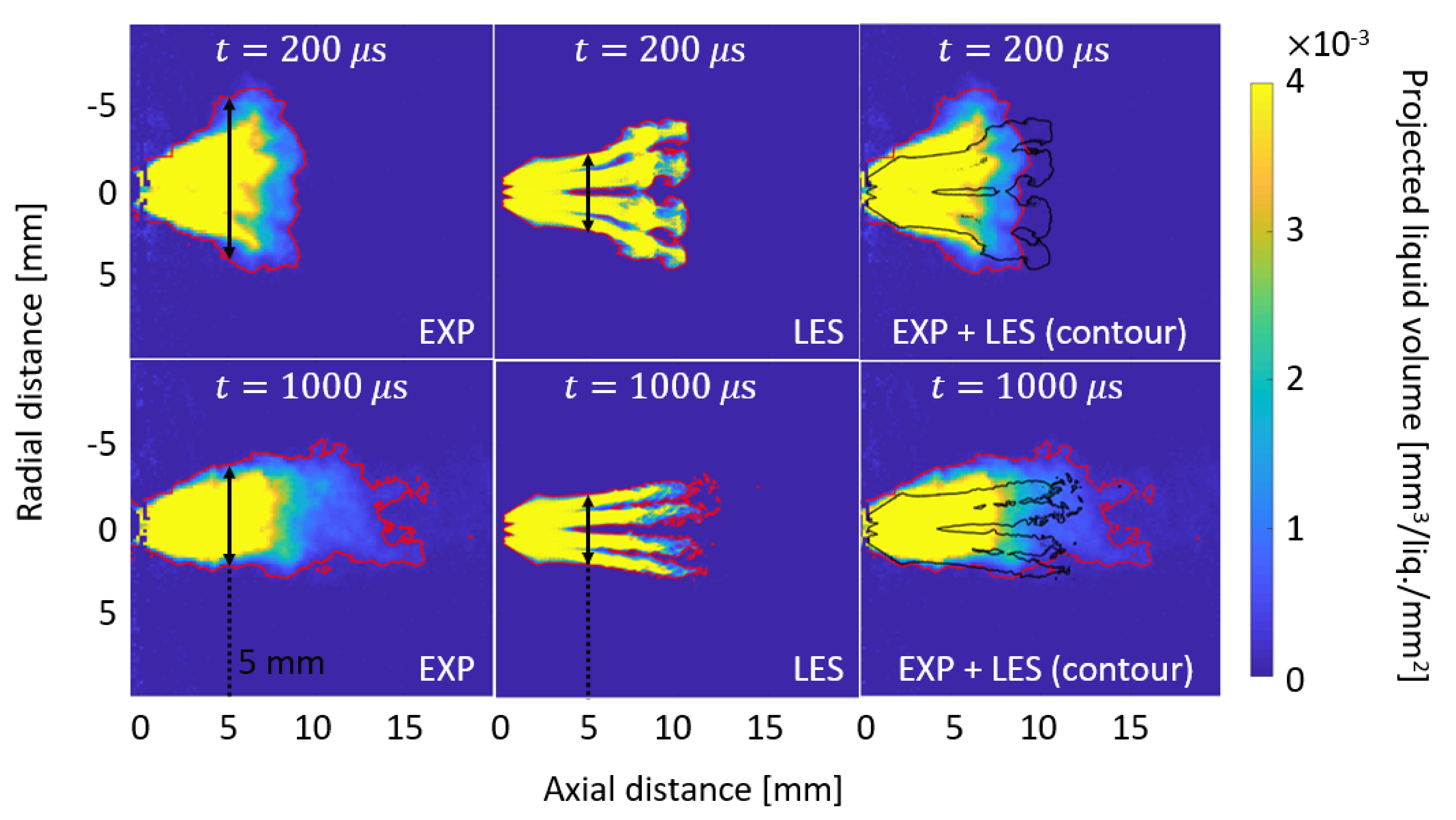
Figure 4 shows the PLV at the early stage of injection (first row) and just before the end of injection (second row) for both the experiments (left column) and the LES (middle column). For a better comparison between the experiments and the LES, the color scale in last column shows the PLV measured in the experiments while the black iso-line shows the liquid boundary in the simulations. The red and black contour lines represent the liquid boundary, defined as $2\times {10}^{-4}{\mathrm{mm}}^3{\mathrm{liq}./\mathrm{mm}}^2$ for both LES and experimental results. The PLV shown in Figure 4 has been realization-averaged over five realizations for both the LES and experiments to ensure that the conclusions made do not depend on a singular event observed in one realization. At 200 $\mathsf{\mu }$s after the start of injection (ASOI), the experiments show strong interaction between the plumes, making it difficult to distinguish the plumes. The LES also show interaction between plumes but to a lesser degree compared to the experiments. The overall structure of the spray is reasonably well captured in the simulations. At 1000 $\mathsf{\mu }$s ASOI it is impossible to distinguish the plumes in the experiments because of the very strong collapse, consequence of the high ambient density. However, in the LES, separated plumes can still be observed, indicating an underestimation of the spray interaction despite the fact that a relatively large cone angle (40${}^{\circ }$) has been imposed as the boundary condition. The plume bending towards spray collapse is quantified by comparing the liquid width at 5 mm from the injector (indicated by the black arrows in Figure 4) between 200 and 1000 $\mathsf{\mu }$s ASOI. In the LES, the liquid spray width is decreased by 13% between 200 and 1000 $\mathsf{\mu }$s, while the experiments show a decrease of 61%. Such observations indicate that the models used in this study only partially capture the physical phenomena leading to spray collapse under these conditions.

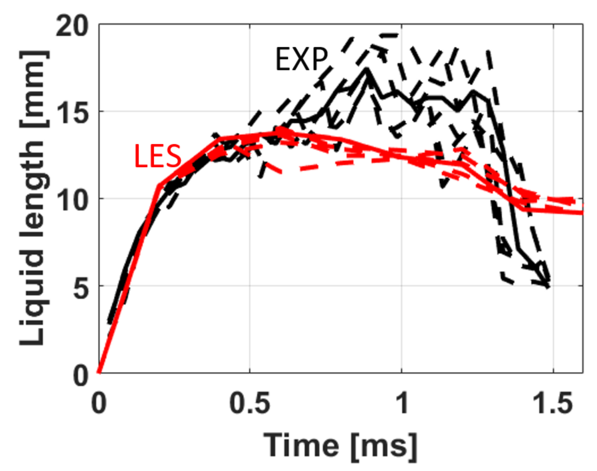
The performance of the simulations can also be evaluated by comparing the liquid-penetration length between the LES results and the experiments as shown in Figure 5. The solid lines represent the liquid length based on the ensemble-averaged PLV, while the dashed lines show the liquid length for individual realizations. For both the LES and the experiments, the liquid length is defined as the furthest distance where there is no break in connected PLV ($2\times {10}^{-4}{\mathrm{mm}}^3{\mathrm{liq}./\mathrm{mm}}^2$ threshold). This definition, called the “main core liquid length” in [26], excludes small pockets of liquid detached from the main core, causing high fluctuation in the liquid length for individual realizations. For both LES and experimental results, the solid lines (ensemble-averaged) seem to be representative of the liquid length observed in individual realizations, indicating that the number of realizations was sufficient for this analysis. During the first half of injection (up to 0.6 ms), the LES are in very good agreement to the experiments. Then, due to the strong collapse observed in the experiments, the liquid length continues to rise in the experiments unlike the simulations. Note that the liquid length differences between the measurement and the simulations are partially caused by the non-symmetric behavior of some plumes in the experiments, which is not modeled. Blessinger et al. [18] using the same injector, had already noticed such behavior, performing side- and front-view Mie-scattering. This asymmetry can be observed in Figure 4 at 1000 $\mathsf{\mu }$s, where the liquid length, at the radial distance +2 mm penetrates significantly more than at the radial distance −2 mm.

In conclusion, Figure 4 and Figure 5 show that the simulations are matching well the experiments during the first half of injection. Then, the simulations under-predict the level of plume-to-plume interaction observed in the experiments, leading to underestimate the liquid length by approximately 3–4 mm. Despite differences observed between LES and experiments, the overall performance of the simulations is judged adequate to represent key features of mixture, such as vaporization and spray collapse. A deeper evaluation of the simulation against the experiments is provided in the section focusing on the combustion.

4. Flame Propagation after Ignition

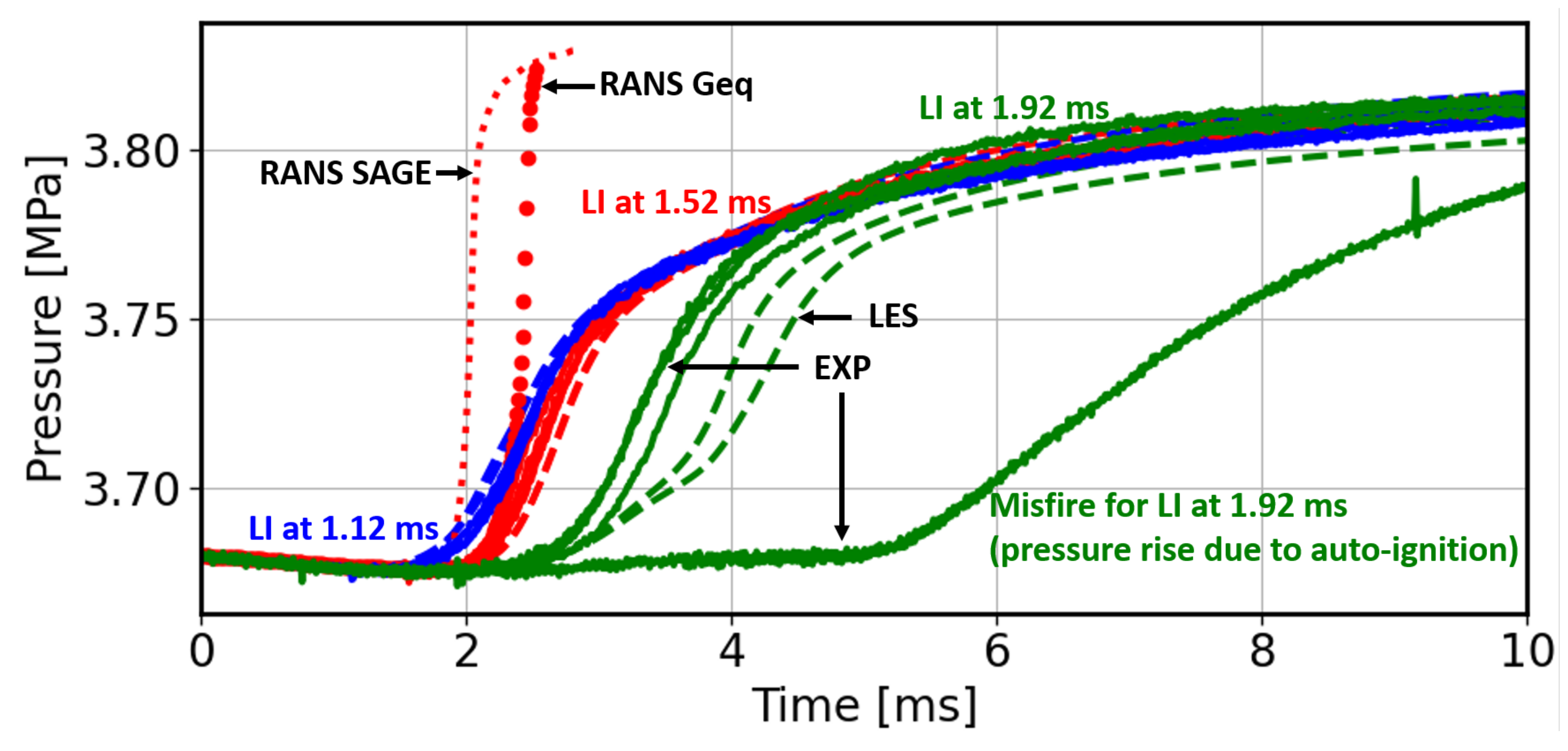
Figure 6 shows the pressure rise in the vessel after ignition at different timings for the experiments and the simulations. The solid lines represent the pressure rise in the experiments, the dashed lines show the LES results and for ignition at 1.52 ms. Moreover two RANS simulations have been performed and are represented with the circular symbols.

For ignition at 1.12 ms (immediately at the end of injection) the LES agree with the experiments at the initial rise in pressure to 3 ms, as well as the slower rise to 10 ms. The fact that the onset, slope, and final value (at 10 ms) of the pressure rise are well captured in the LES indicates that the mixture and the ignition source are well predicted in the simulations. More details justifying these claims will be provided later in the article. The realization-to-realization variability is low for both LES and experiments, generating confidence that the simulation can be used with reliability to interpret the experiment.

Similar success in LES heat release fidelity is demonstrated for the ignition at 1.52 ms (0.4 ms after the end of injection). The delayed heat release essentially catches up to the 1.12 ms ignition case by approximately 3 ms. By contrast to the LES, two RANS simulations show huge disparities compared to the experiment. The RANS simulations include one with the SAGE combustion model [31] (identical numerical setup as our previous study [16]) and another with the G-equation combustion model developed for premixed flame applications [38]. Both RANS simulations largely overestimate the pressure rise, with very fast flame propagation and large total burned charge. The main culprit, regardless of the turbulent combustion model being employed, can be explained using the following turbulent flame speed correlation [39]:

$$S_t=S_l+u^{\prime }\left(-\frac{a_4{b}_3^2}{2b_1}Da+{\left[{\left(\frac{a_4{b}_3^2}{2b_1}Da\right)}^2+a_4{b}_3^{2}Da\right]}^{1/2}\right)$$

(3)

where $s_t,s_l$ is the turbulent and laminar flame speed, respectively. $a_4,b_1,b_3$ are modeling constants. $Da$ is the turbulent Damkohler number, defined as

$$Da=\frac{s_l{l}_t}{u^{\prime }{\delta }_l},$$

(4)

where $l_t$ is the resolved turbulent length scale, and ${\delta }_l$ is the laminar flame thickness. In both equations above, $u^{\prime }$ is the turbulent fluctuating velocity. For the current scaling analysis, we can assume $u^{\prime }$ is the same in both LES and RANS. For a given fuel and thermodynamics conditions, both flame speed and thickness are also assumed constant. Then, the turbulent flame speed is simply a function of the Damkohler number, which in turn is a function of the resolved turbulent length scale. In the current RANS calculation, such characteristic length scale is in the order of the integral length scale [40] and can be computed based on RANS theory as

$$l_t=c_{\mu }^{3/4}\frac{k^{3/2}}{ϵ},$$

(5)

with $ϵ$ the turbulent dissipation and $c_{\mu }$ is equal to 0.09. Using Equation (5), the resolved scale in the RANS simulations at the time of ignition is 321 $\mathsf{\mu }$m. The turbulent length scale resolved in an LES model is the size of the filter width, which is 62.5 $\mathsf{\mu }$m in this work. It should be reiterated that the turbulent length scales computed in the above analysis are the ones resolved by the simulations and should not be confused as the real physical turbulent length scale of the problem. The above analysis indicates that the turbulent flame speed is significantly overestimated in the RANS calculation compared to LES. Because we can treat any reactive scalar in the SAGE model as a progress variable where the mean flame front propagates according to the turbulent flame speed correlation in Equation (3). Therefore, the scaling argument above is applicable to both the SAGE as well as G-equation model. Furthermore, the agreement with the experiment throughout both the early-burn and late-burn stages is strong evidence that the LES coupled to standard well-stirred combustion model (SAGE) is much more accurate than RANS simulations (using G-equation or SAGE). It echoes Xu et al. [11] engine simulations, where they observed an overestimation of heat release in RANS when the mixture is ignited during the pilot injection. Simulations using a LES turbulence model did not show such overestimation. While it has become common to tune parameters in a G-equation formulation [10,11] to match heat release, results here show that this practice is not predictive, as the variation in modeling constants is not motivated by any physical phenomena. In this experimental case, injection velocities and turbulence are particularly high immediately at the end of injection, thus exacerbating this RANS/combustion model shortcoming. Fortunately, the use of Dynamic Structure LES and a well-stirred reactor combustion model appears to be an adequate solution.

Rounding out the ignition timing variation, experiments for the late-ignition case at 1.92 ms (0.8 ms after the end of injection) showed delayed but adequate heat release for some realizations, but also complete misfire in one realization. The ignition (with nanosecond laser ignition) at this timing is therefore highly variable and unstable but understanding the different realizations and underlying reasons for success or failure has merits. Notably, the LES predict heat release intermediate to experiments, although with less variability than the experiments. Nevertheless, the overall realization-to-realization variability for the LES events does increase, in consistency with the experiments. Such higher variability is expected since after the injection the mixture is more subjected to random fluctuation, presenting mixtures at the ignition location that are progressively more fuel lean.

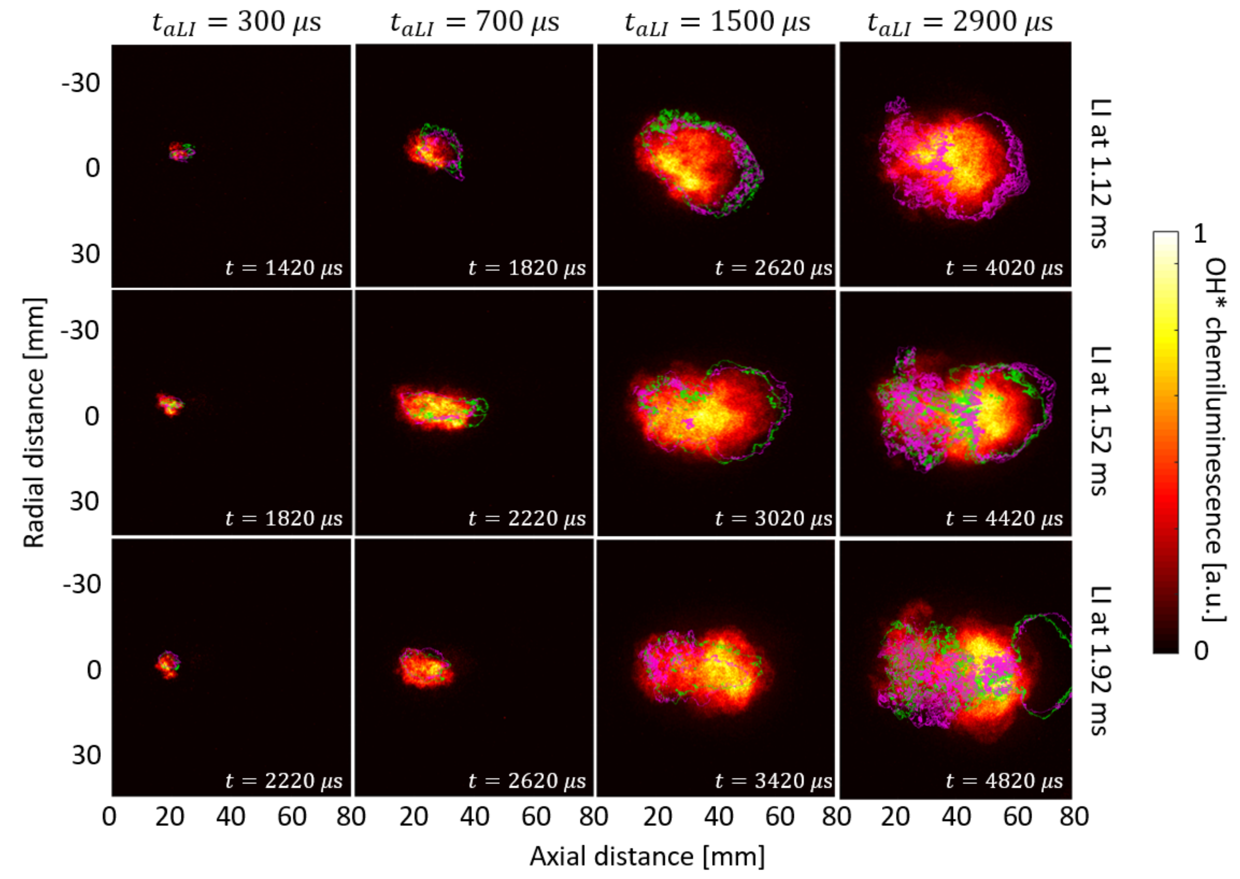
A deeper analysis of the flame behavior is presented in Figure 7. The color scale shows the ensemble-averaged normalized OH* chemiluminescence signal for ignition at different timings (experimental setup described in [16]). In order to perform an accurate comparison to the experiments, OH* reactions have been added to the Liu chemical mechanism. One-D premixed flame calculations confirmed that adding OH* into the chemistry did not alter the flame speed. OH* mass fraction has been integrated in the y direction and projected onto the X–Z plane using the same method as projected liquid volume to mimic the line-of-sight measurement. The resulting flame boundary is shown with the magenta and green isolines in Figure 7. The two different colors correspond to two different realizations. At 300 $\mathsf{\mu }$s after Laser Ignition ($t_{aLI}=300\mathsf{\mu }$s) the LES and the experiments show a small flame kernel in vicinity of the ignition source (~3 mm above the injector and 17.4 mm downstream) for all the cases. At 700 $\mathsf{\mu }$s after ignition, both LES and experiments show that the flame is accelerating and moving in the center of the jet where the flow velocity is higher; 800 $\mathsf{\mu }$s later (at 1500 $\mathsf{\mu }$s) the flame continues to expend radially and axially. Generally, at the timing of 1500 $\mathsf{\mu }$s the shape of the projected flame is well captured in the 1.12- and 1.52 ms ignition simulations, in terms of both the axial and radial shape and penetration. However, for the late ignition case (1.92 ms), the LES underpredict the radial expansion of the flame, and the predictions also show axial expansion greater than the experiment, suggesting some mismatch in charge position or flame. At 2900 $\mathsf{\mu }$s after ignition, the simulations with early ignitions (1.12 and 1.52 ms) continue to match the experimental measurement. Note that only small differences are observed between different LES realizations for the same case. For late ignition, the trend observed at $t_{aLI}=1500\mathsf{\mu }$s, continues to be manifest at $2900\mathsf{\mu }$s: the flame in the LES propagates too fast in the head of the jet and does not consume the mixture radially as much as observed in the measurements. The underestimation of the radial expansion (and thus flame volume) leads to an under-prediction of the heat release, compared to successfully ignited experimental cases. Therefore, the predicted pressure rise is lower than the burning experimental cases in Figure 6.

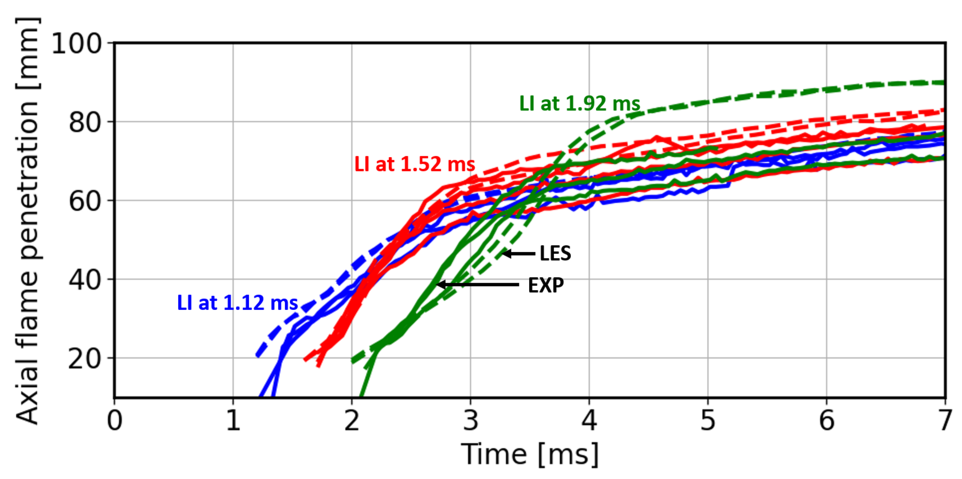
Figure 8 shows observations of the flame axial flame penetration (defined as the farthest axial position of the flame) quantitatively as function of time for different laser ignition timings. Multiple realizations are shown for both the experiments and the LES. The LES results for ignition at 1.12 and 1.52 ms agree with the experiments as has been discussed above. For late ignition (1.92 ms), the axial flame penetration is first underestimated in the simulations. Then, after 0.35 ms, the simulations overshoot the experiments confirming what observed in Figure 7. The simulations are able to capture the two different regimes identified by the slope change in Figure 8 and already observed in [16].

Figure 7 and Figure 8 demonstrated excellent agreement between LES and the measurements in terms of global heat release and flame structure in time for laser ignition at 1.12 and 1.52 ms. It indicates that the mixture preparation as well as the ignition source have been correctly modeled for these cases. However, comparing the successful combusting experiments, when ignition is performed 0.76 ms after the end of injection (1.92 ms ASOI), the flame topology does not exactly match, as discussed above. It is important to note that, for this condition, in the experiments many laser ignition attempts failed, while for the two LES realizations performed, both were successfully ignited. Possibly, the source term modeled in the LES is too powerful and ignites the charge for local mixture which was impossible to ignite in the experiments (too lean). This mismatch in ignition volume is a known problem for experiments and simulations in the lean limit, and it can generate a flame in the LES that does not occur in the experiments. If this theory is correct and the realization-to-realization variation is similar between experiments and LES, we could expect a better agreement to the experiments performing a larger number of simulations.

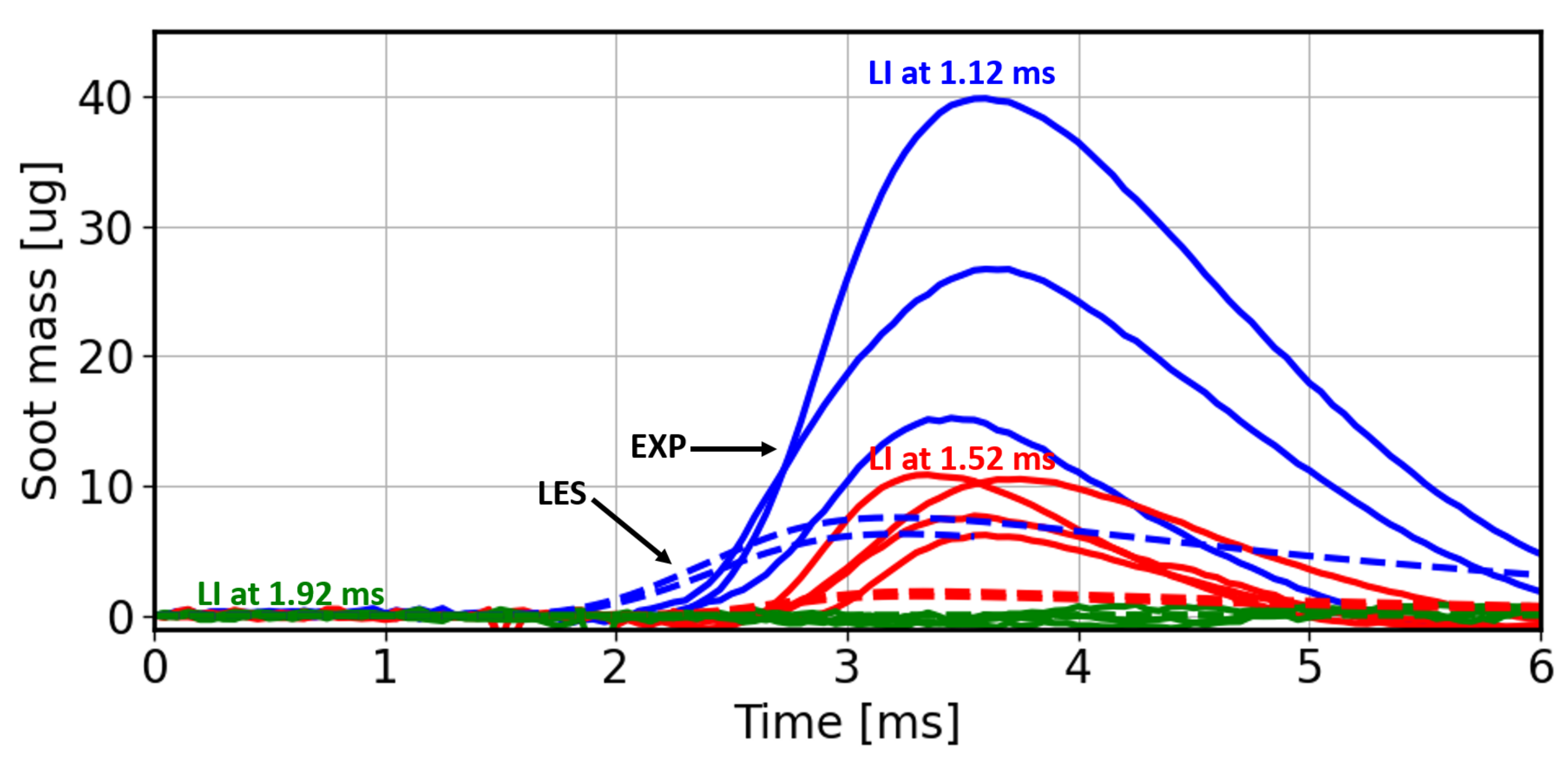
5. Soot Formation and Oxidation

The soot formation and oxidation from the LES, using the empirical Hiroyasu-NSC (Nagle and Strickland–Constable) soot model [36], is compared to the experimental measurement in this section. Figure 9 shows the total soot mass in the vessel as function time for all three ignition timings. Following the same illustration methodology as in Figure 6 and Figure 8, the solid lines indicate different realizations from DBI measurement while the dashed lines represent the simulations. Comparing the experiments and the simulations, it appears that the time of peak soot in the LES is in fair agreement to the measurement, as indicative that mixing of oxygen is also correctly modeled. However, for early ignition, the simulations largely underestimate the maximum soot concentration measured. Furthermore, the soot onset timing is advanced in the LES compared to the measurement. The same observations made for early ignition are also true for ignition at 1.52 ms: underestimation of the maximum soot concentration and over-prediction of the soot onset in the simulations. The empirical Hiroyasu-NSC soot model uses acetylene as soot precursor, which is a significant simplifying assumption. Studies show [41] that larger soot precursors (not available in the mechanism used) are better candidates to model accurately the Polycyclic Aromatic Hydrocarbons (PAH) and soot formation. As PAH molecules are formed after acetylene, using PAH molecules as a soot precursor is expected to delay the soot formation and, therefore, better match the experiments. Interestingly, the experiments show high realization-to-realization variation in terms of soot prediction while the global pressure rise (Figure 6) and axial flame penetration (Figure 8) did not show this phenomenon. Such variation is indicative of local variances in rich mixture from realization-to-realization. Such high realization-to-realization variation was not observed in the LES as illustrated with the dashed lines in Figure 9.

Finally, for laser ignition at 1.92 ms Figure 9 shows that the LES do not predicate significant level of soot as observed in the measurement for laser ignition at 1.92 ms.

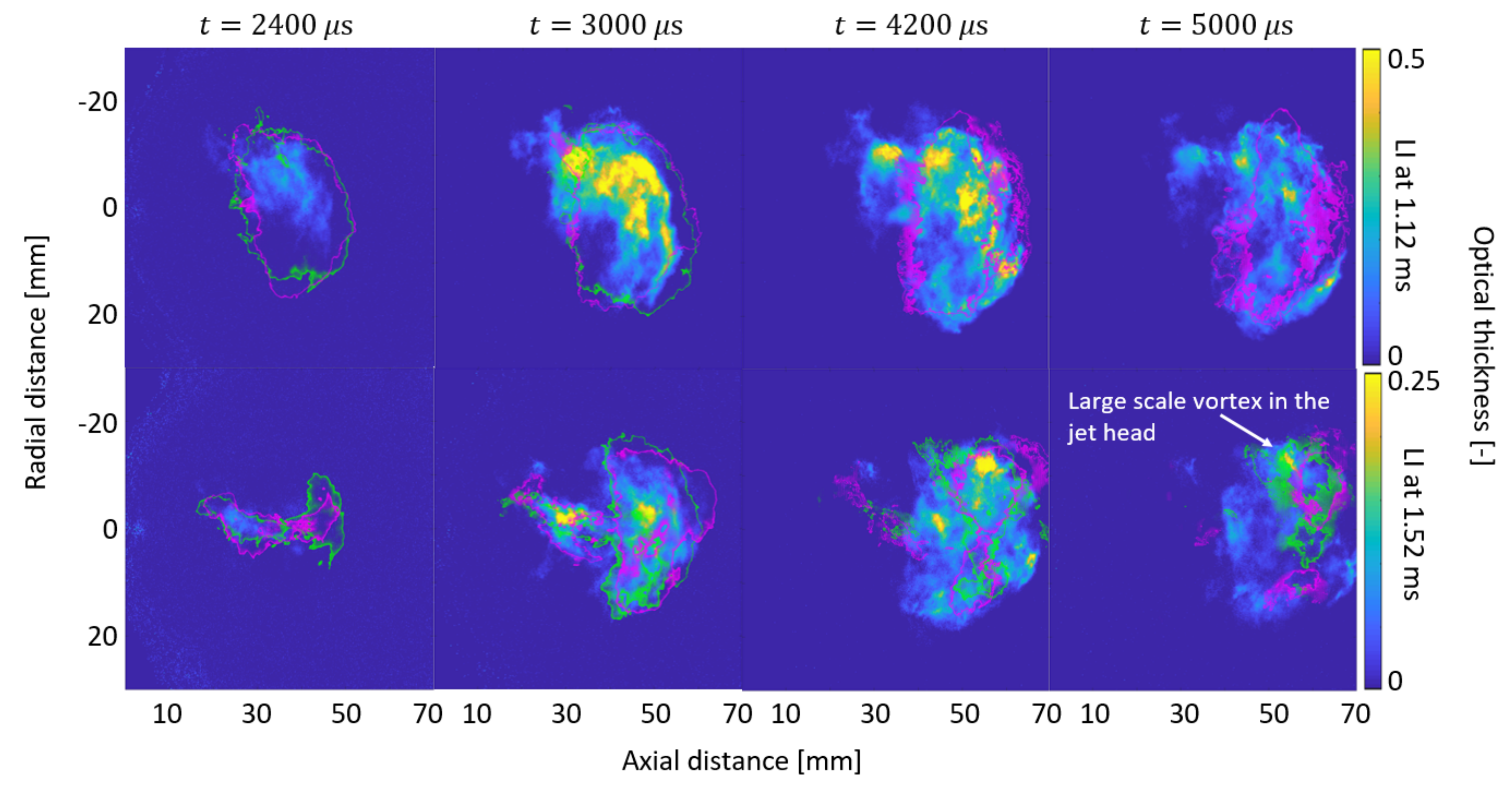
The color scale in Figure 10 shows ensemble-averaged temporal images of optical thickness (proportional to soot mass), for laser ignition at 1.12 and 1.52 ms. Following the same methodology as developed for Figure 7, the soot concentration in the computational domain has been integrated in the y direction and projected onto the X–Z plane to mimic the line-of-sight measurement. The resulting soot cloud boundary from this processing is shown with the magenta and green isolines in Figure 10. The two different colors corresponding to two different realizations.

For early laser ignition (1.12 ms), the measurements and the simulations show that the soot formation starts radially offset from the injector (−5 mm). Then, the soot cloud moves toward the injector axis. At 2400 $\mathsf{\mu }$s ASOI the simulations slightly overestimate the size of the soot cloud, which is consistent with the early soot prediction observed in Figure 9. From 3000 to 5000 $\mathsf{\mu }$s, the soot boundary predicted in the simulations are in good agreement with the experiments.

For laser ignition at 1.52 ms, high soot concentration is first detected on the injector axis, the presumed result of rich fuel–air pockets consumed by the flame. The LES are able to capture correctly the shape of the soot cloud starting at 15 mm downstream of the injector, including the large-scale vortexes at the head of the jet. From 4200 to 5000 $\mathsf{\mu }$s, the optical thickness measurement shows a decrease in soot due to oxidation at high temperature and within mixture fractions that are progressively more lean and abundant with oxygen. The last region where soot can be observed, for both experiments and LES, is at the head of the jet in the large-scale vortexes.

In conclusion, a comparison of the soot formation/oxidation processes between the measurements and the LES revealed that the Hiroyasu-NSC soot model captured accurately the structure of the soot cloud. However, the simulations failed to match the experiments quantitatively. The high-temperature flame analysis, detailed in the previous section, showed that the LES matched well the measurements (for ignition at 1.12 and 1.52 ms). As the topology of the flame and heat release closely matches the experiment, we have strong reason to conclude that the mixture is well captured in the simulations, and the differences observed in soot formation are coming from the soot modeling. A more accurate prediction of soot is expected using more realistic soot precursors in the chemical mechanism and as inputs in the soot model, as well as using a detailed soot model (the sectional methods can be found, for example, in [42,43,44]).

6. Fuel-Air Mixture Analysis

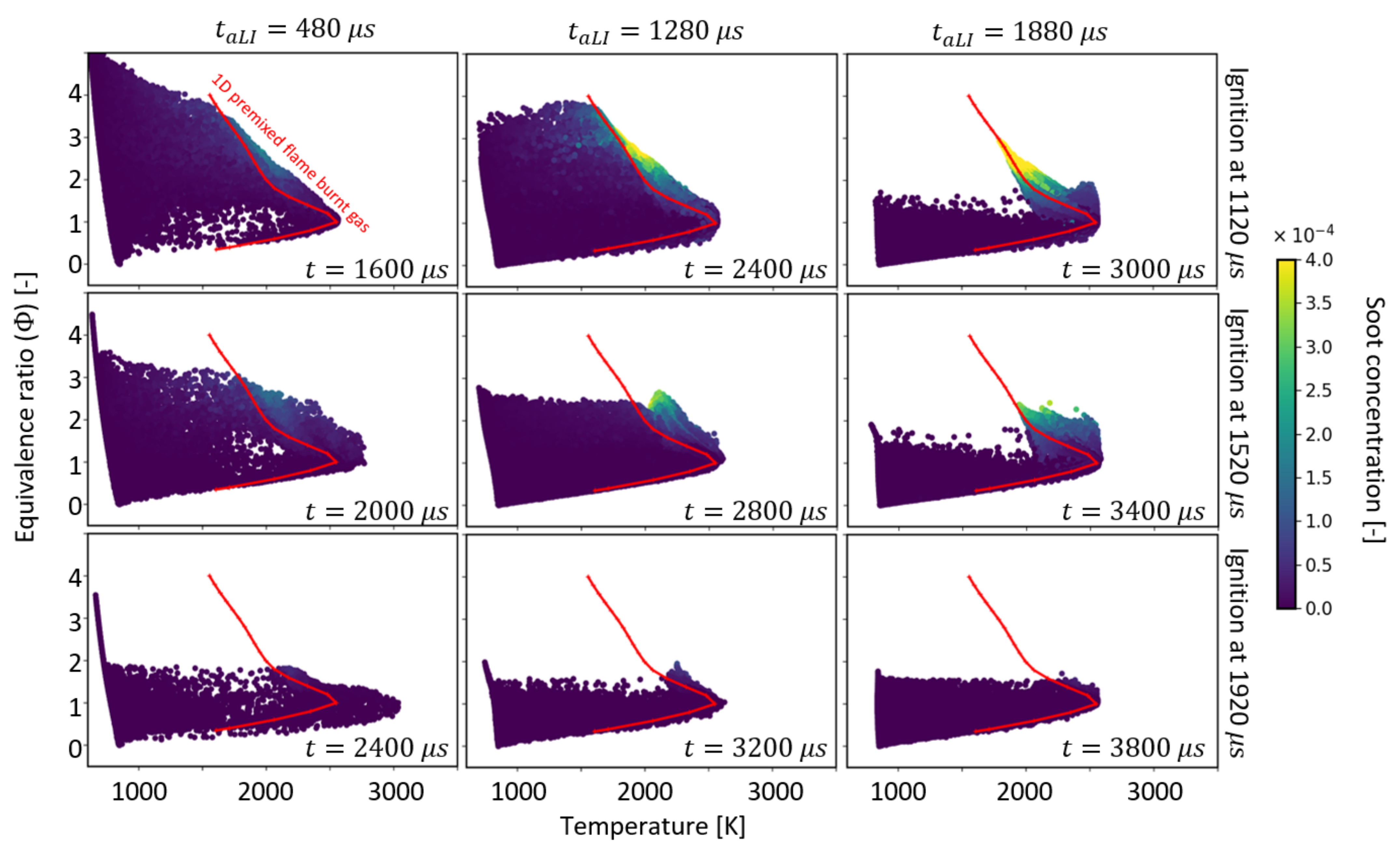
Because the LES show strong indicators that mixture is adequately predicted, we seek to capitalize on this success to better understand the critical evolution of mixture and how this affects soot and overmixed regions as sources of combustion inefficiency. The fuel–air mixture after ignition is first analyzed by plotting the equivalence ratio as a function of the temperature in Figure 11. The equivalence ratio ($\mathsf{\Phi }$) is a passive scalar, independent of the reaction state (same definition as in [16]). The points in the scatter plots are colored by the soot concentration, which is defined as the soot mass divided by the total gaseous mass in the Eulerian grid. In addition, the red curves show the burnt gas temperature from 1D premixed flames where the fresh gas temperature is determined assuming an adiabatic mixing, like shown in Figure 3. Note that some points largely exceed the maximum 1D flame temperature (2500 K) just after ignition. These cells are localized at the ignition site, where the energy source term considerably increases the temperature.

Immediately after ignition ($t_{aLI}=480\mathsf{\mu }$s), the flame propagates in very rich mixture ($\mathsf{\Phi }>4$) for ignition at 1.12 ms. Such observation is also true for ignition at 1.52 ms, where high-temperature reactions can be seen up to $\mathsf{\Phi }$ = 3.5. At this stage, the soot concentration is low for both laser ignition timings. For late ignition (1.92 ms), the fuel has more time to mix with the ambient gas. Therefore, even 480 $\mathsf{\mu }$s after ignition, the flame does not consume mixture greater than 2. Moreover, the scatter plot shows a high concentration of points at the stoichiometric mixture ($\mathsf{\Phi }=1$) indicating high combustion efficiency.

At $t_{aLI}=1280\mathsf{\mu }$s high soot concentration is observed for rich mixture and high-temperature, which is in agreement with the “soot island” representation available in the literature [45]. The maximum soot concentration is identified at $\mathsf{\Phi }=3$ and $T=2000$ K, corresponding to the optimal condition to form soot. Higher temperature resulting in soot oxidation, while richer mixture does not allow sufficient temperature for the soot to develop. When ignition is performed at 1.52 ms, the optimal region for soot cannot be reached because of the leaner mixture available, resulting in less soot produced. In this case, the maximum soot concentration is observed at $\mathsf{\Phi }=2.5$ and $T=2100$ K. For ignition at 1.92 ms, no soot is observed and the mixture consumed by the flame is mainly fuel lean and stoichiometric.

Finally, $t_{aLI}=1880\mathsf{\mu }$s represents the soot mass peak in Figure 9 for ignition at 1.12 and 1.52 ms. In both cases, the mixture being consumed by the flame is now below $\mathsf{\Phi }=2$ as indicated by the absence of points in the scatter plot between $T=850$ K and the 1D burnt gas temperature at $\mathsf{\Phi }=2$. The maximum soot concentration is located on the 1D premixed flame burnt gas curve. Because there is no rich mixture to burn, the soot production first stops, and then soot is oxidized, as shown in Figure 9.

Figure 12 spatially illustrates the relation between rich mixture, high-temperature flame, and soot formation observed in Figure 11. The black ($\mathsf{\Phi }=1$) and green ($\mathsf{\Phi }=2$) isolines help to visualize the mixture preparation. We highlight $\mathsf{\Phi }=2$ because previous studies have shown that the soot production can be avoided if combustion occurs at premixed $\mathsf{\Phi }<2$ [45,46,47,48,49].

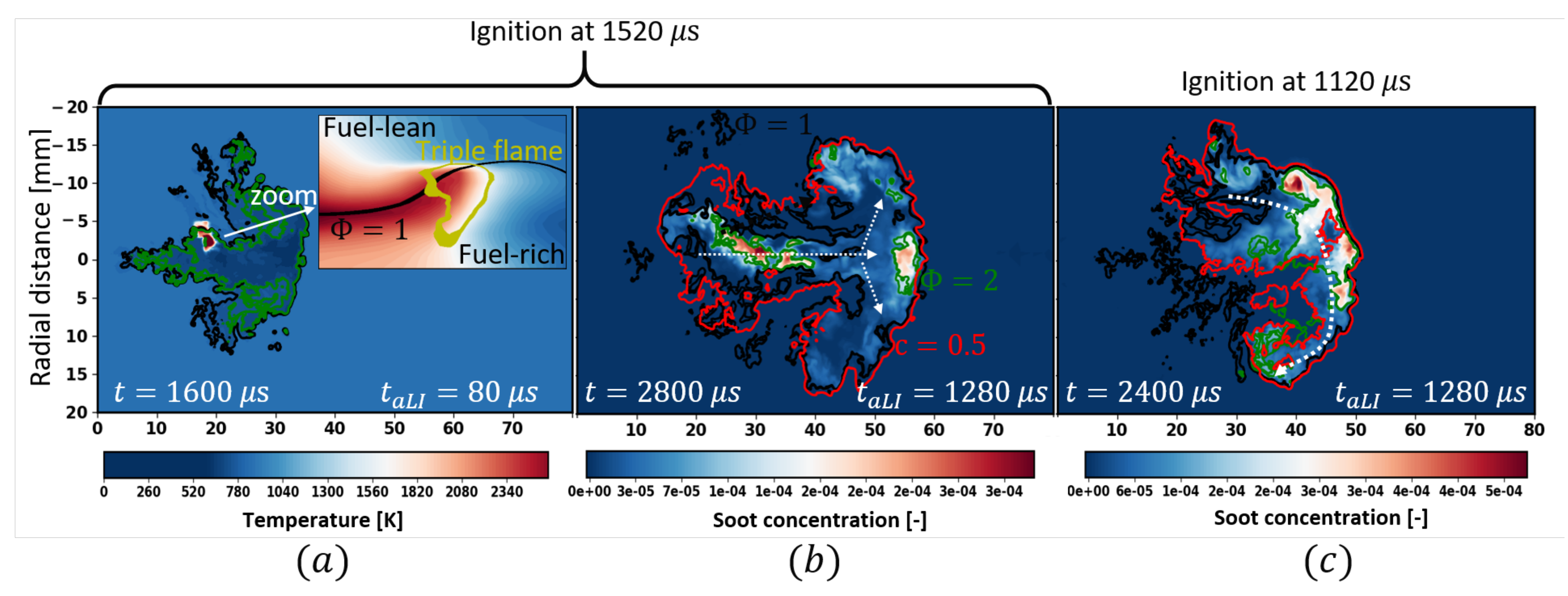
Figure 12a shows an axial slice of the temperature at 80 $\mathsf{\mu }$s after ignition (for ignition at 1.52 ms). Due to the strong spray collapsing caused by the high-density condition, a rich mixture is clustered in the center of the injector axis, even though the fuel comes from an 8-hole symmetric injector with no plume directly targeting the injector axis. This example illustrates that strong spray collapse can significantly change the mixture preparation compared to low-density (and non-flashing) case where the mixture follows the nozzle axis. Figure 12a also illustrates the flame just after ignition, which is centered on the stoichiometric line. Featuring the ignition zone in a zoomed-in region, a triple flame [50] can be observed, as illustrated by plotting the heat-release rate iso-line in yellow. The three characteristic branches of triple flames can be observed [50]: a rich premixed flame, a lean premixed flame and, in between, a third branch, which is a diffusion flame situated on the stoichiometric line. Triple flames are observed in stratified mixture when the flame encounters at the same time fuel-lean, rich, and stoichiometric mixture. Xu et al. [11] identified a triple flame while performing LES engine simulations for mixed mode combustion.

Figure 12b shows the soot concentration at 1280 $\mathsf{\mu }$s after ignition. The flame boundary (illustrated with the red isoline) is defined using a progress variable ($c=0.5$) [39], computed using the following equation:

$$c=(T-T_{amb})/(T_{burnt}-T_{amb}),$$

(6)

where T is the temperature in the Eulerian cells, $T_{amb}$ is the ambient temperature in the vessel (850 K), and $T_{burnt}$ is the burnt gas temperature (2500 K). The flame dynamic over time is illustrated by the dashed white arrows. The flame first propagates along the injector axis where the flow velocity is high, reaching the head of the jet as illustrated with the horizontal arrow. Then, the flame propagates into the large-scale vortices where there is still fuel available for combustion. The high soot concentration pockets are localized in the burnt gases, in fuel-rich regions encircled by the green isoline (indicating mixture richer than $\mathsf{\Phi }=2$). These pockets are localized near the ignition location at ~25 mm from the injector and at the head of the jet.

Figure 12c shows the soot concentration at the same time after ignition as image (b) (1280 $\mathsf{\mu }$s), but for early ignition. The flame dynamic is different compared to ignition at 1.52 ms as shown with the dashed arrows. For early ignition, the mixture is more radially expended at the 17.4 mm from the injector (axial location of ignition spot). As a result, the flame first consumes the fuel available far from the injector (radially). Then, the flame propagates at the periphery of the main charge reaching the rich mixture at the head of the jet and, ultimately, crossing the injector axis to consume the rest of the fuel available on the other side. Therefore, in this case, the high soot concentration pockets are not localized in the jet axis near the ignition location but at the head of the jet where the mixture is fuel-rich. As observed in the scatter plot Figure 11, the soot production at 1280 $\mathsf{\mu }$s for ignition at 1.12 ms is much higher than the one at 1.52 ms. Note that in Figure 12c the maximum of the color scale is increased (compared to image (b)) to avoid saturation.

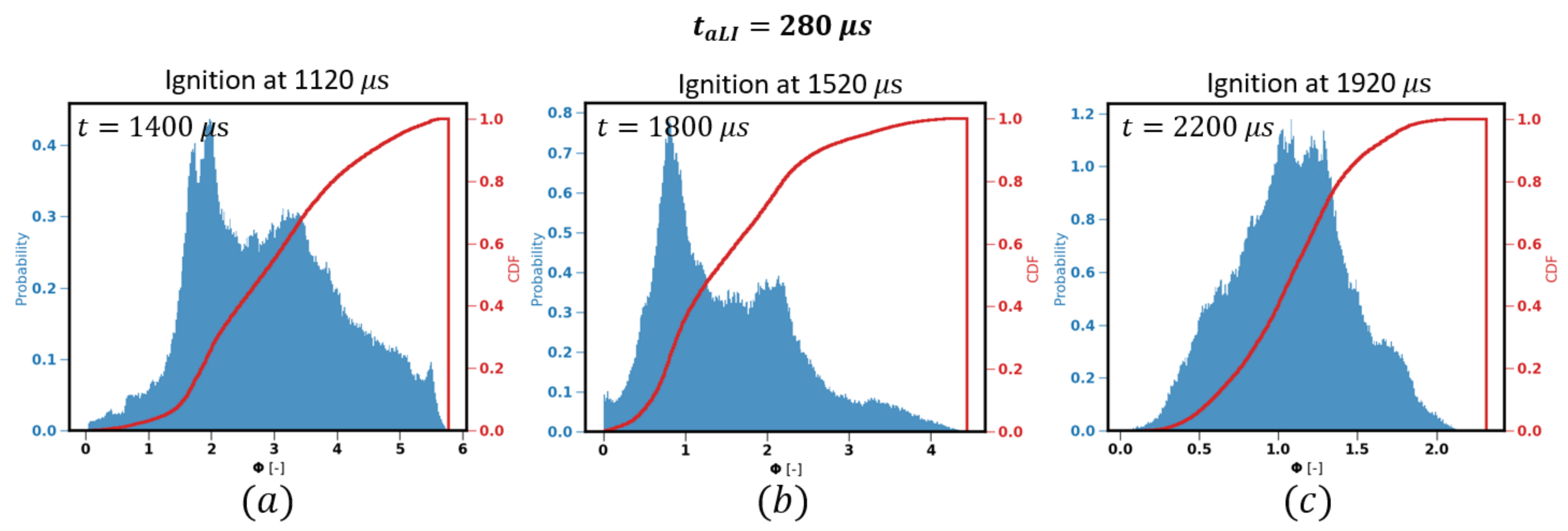
Tracking the Mixture Consumed by the Flame

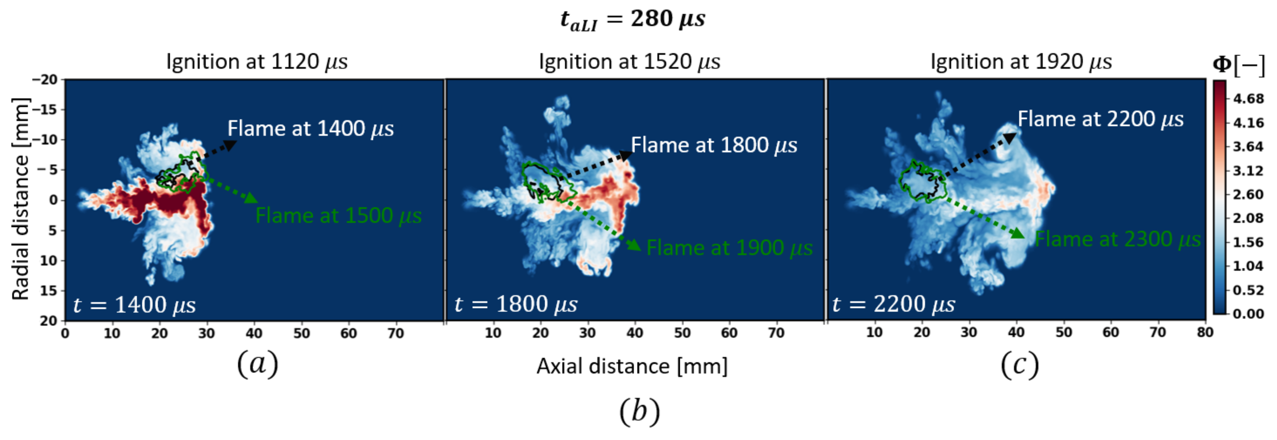
In this last section, we track in time the mixture consumed by the flame for the different laser ignition timings. One objective of this analysis is to understand how to successfully propagate a stratified flame, but to avoid soot formation. Figure 13 shows a slice of the equivalence ratio at 280 $\mathsf{\mu }$s after ignition. On each image two lines are plotted: the black line represents the flame boundary (defined by $c=0.5$) at $t_{aLI}=280\mathsf{\mu }$s (time matching $\mathsf{\Phi }$ in slice) while the green line shows the flame boundary 100 $\mathsf{\mu }$s later. Taking the early ignition case as example (Figure 13a), the mixture consumption between 1400 and 1500 $\mathsf{\mu }$s is defined by extracting $\mathsf{\Phi }$ at 1400 $\mathsf{\mu }$s in between the flames at 1400 and 1500 $\mathsf{\mu }$s. This postprocessing technique assumes that the flame consumes the mixture instantly within the time step of 100 $\mathsf{\mu }$s (time resolution corresponding to the 3D outputs frequency). Such assumption will be discussed later in the article. For the sake of clarity, the methodology is illustrated in slices but the post-processing is applied to the full 3D flame.

Figure 14 shows the equivalence ratio distribution in the 3D domain corresponding to the time shown in Figure 13. For early ignition (Figure 14a), the $\mathsf{\Phi }$ probability peaks at $\mathsf{\Phi }=2$, and the cumulative distribution function (CDF), in red, indicates that 75% of the mixture consumed by the flame is richer than $\mathsf{\Phi }=2$, representing a great potential for soot. This value drops to 27% for ignitions at 1.52 ms. However, the rich mixture ($\mathsf{\Phi }>3$) in the center of the jet is still observed and will participate in the soot formation process. Finally, for late ignition, the mixture is more homogeneous and the equivalence ratio is below 2. Consequently, almost no soot is formed as shown in Figure 9. This result is in agreement with previous studies [45,46,47,48,49] where it has been found that soot is not formed if the flame consumes mixture leaner than $\mathsf{\Phi }=2$.

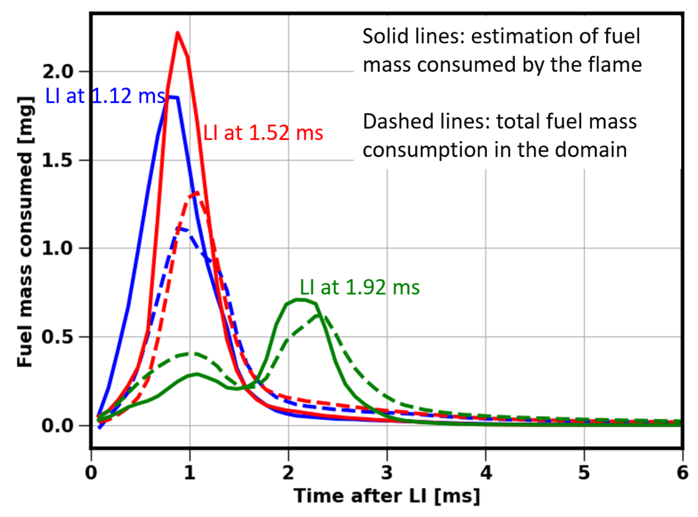
Before using our postprocessing technique to estimate the equivalence ratio and fuel mass consumed by the flame for further analysis, it is important to evaluate the error resulting from the simplifying assumptions. Extracting the mixture information at a time $t_0$ based on the flame movement between $t_0$ and $t_1$ (where $t_1-t_0=100\mathsf{\mu }$s) implies that when the flame propagates the flow between $t_0$ and $t_1$ is frozen. Figure 15 is used to evaluate such assumption. The dashed lines show the total fuel mass consumption in the domain, while the solid lines show the fuel mass consumed by the flame using our postprocessing technique. For laser ignition at 1.12 and 1.52 ms, the fuel mass consumption is first overestimated using the flame tracking technique. For these early ignition timings, the flame propagates in regions where the flow velocity is high and the rich mixture is located at the head of the jet as shown in Figure 13. Therefore, when the flame propagates in the jet head direction, the downstream portion of the mixture identified as being consumed may not be consumed because of flow convection, resulting in overestimation of the fuel mass consumed by the flame. Because of lower flow velocity for late laser ignition, the fuel mass consumed by the flame is much closer to the total fuel mass consumption (green curve) compared to the early ignition timings. After the peak of fuel mass consumption, Figure 15 shows that the fuel mass consumed by the flame is lower than the total fuel mass consumption in the domain. This can be explained by the low-temperature reactions occurring outside of the high-temperature flame, responsible for breaking is-octane into intermediate species at low temperature (e.g., 1200 K).

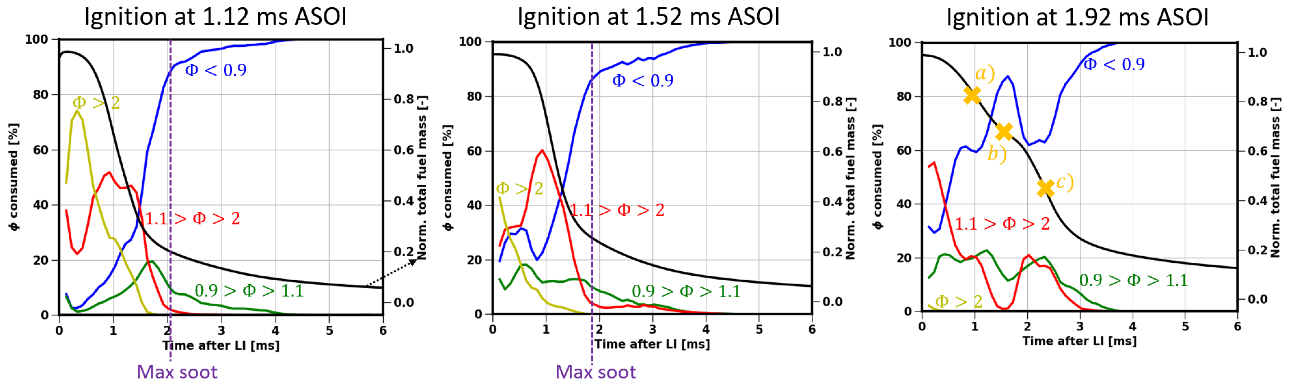
Figure 16 (colored curves) shows the equivalence ratio consumed by the flame on the left y-axis as a function of the time after laser ignition. The equivalence ratio is binned into four groups: mixture richer than $\mathsf{\Phi }=2$ representing high potential for soot (yellow), rich mixture between 1.1 and 2 (red), stoichiometric (green) and lean (blue) mixture. Figure 15 showed that the methodology used to track the mixture consumed by the flame might over-estimate the fuel mass consumption due to rich-fuel pockets unduly taken into account. Therefore, the results in Figure 16 are analyzed with caution when the deviation between the solid and dashed lines in Figure 15 are high, which is mainly during the early flame growth for laser ignition at 1.12 and 1.52 ms.

For early laser ignition, the equivalence ratio consumed by the flame is mainly fuel-rich until 1.5 ms after LI (time when the lean mixture becomes dominant), resulting in fast decrease of the normalized total fuel mass (black curve using the y-axis on the right). At 1.5 ms after LI, 68% of the fuel mass injected has been consumed. Then, the flame consumes stoichiometric (up to 20% of the mixture is at $\mathsf{\Phi }=1$ at 1.7 ms) and fuel-lean mixture. Less than 1% of the total fuel remains in mixtures where combustion is totally fuel-lean.

Similarly for ignition at 1.52 ms, a rich mixture is first consumed. In this case, the maximum percentage of $\mathsf{\Phi }>2$ consumed by the flame is 43%, compared to 74% for early ignition. Moreover, for ignition at 1.52 ms, 56% of the fuel mass injected has been consumed when the fuel-lean consumption becomes dominant, which is 12% less than the early ignition case.

The normalized total fuel mass curve for late ignition behaves differently from the two other cases. For late ignition, the black curve first shows a relatively low fuel consumption rate (indicated by the mark $a)$ in Figure 15 right). During this stage, the mixture consumed is mainly lean (60% lean, 20% stoichiometric, and 20% rich). Then, the flame momentarily propagates in regions where there is no rich mixture ($\mathsf{\Phi }<1.1$) (marked as $b)$), resulting in a decrease of the fuel consumption rate. In region $c)$, the flame again encounters fuel-rich mixture, as shown by the decrease of the blue curve and the increase of the red curve. The fuel consumption rate, in region c, is at the highest level for this case. Finally, all the fuel left is lean, resulting in a slow decrease of the fuel mass, as observed for the other cases.

Figure 16 also shows (vertical dashed purple lines) the time of soot peak extracted from Figure 9. For laser ignition at 1.12 and 1.52 ms, it is interesting to observe that even when the equivalence ratio is below 2, soot are still formed for a short period time. As discussed in [16], soot can continue to grow even if $\mathsf{\Phi }<2$ because of further mixing with hot combustion products, and will only decrease when approaching the oxidizing diffusion flame. However, when the equivalence ratio consumed by the flame is always below 2, no soot is formed, as shown in Figure 9 and Figure 15.

7. Conclusions

Large-eddy simulations of an 8-hole GDI spray have been used to gain better understanding of the ignition, flame propagation and soot formation/oxidation processes under conditions relevant to mixed-mode combustion. Compared to our previous RANS simulations [16], significant improvements have been found in predictability when using a Dynamic Structure LES turbulence model [17] in simulations, coupled with a reduced mechanism. The modeling weakness in RANS is attributed to artificially high flame speed induced by very high turbulent kinetic energy, consequence of ignition in the turbulent GDI spray.

A detailed comparison of the simulations and the experiments showed that the LES were able to capture correctly the liquid penetration length, and to some extent, a degree of spray collapse demonstrated in the experiments. Then, following the same methodology as employed in the experiments, the mixture has been ignited at various times after the end of injection. For early and intermediate ignition timings, the LES showed excellent agreement to the measurements in terms of flame structure, extent of flame penetration, and heat release rate. The soot formation/oxidation was also compared to the experiments, and revealed that the soot location from the simulations was well captured in the LES. However, the soot mass was largely under-estimated using the empirical Hiroyasu model [36].

In order to explain the different flame propagation speeds and soot production tendencies when varying ignition timing, a mixture analysis has been performed by dynamically extracting and analyzing the fuel mass and equivalence ratio ($\mathsf{\Phi }$) being consumed by the flame. When ignition is performed immediately at the end of injection, the mixture consumed by the flame is dominated by fuel-rich mixture ($\mathsf{\Phi }>2$) until 0.7 ms after ignition. Delaying ignition by 0.4 ms, reduced the soot production by 80%. The mixture consumed by the flame is significantly leaner than the early ignition. For late ignition, the equivalence ratio burned by the flame is never greater than 2, resulting in no significant soot production as observed in the experiments.

Despite the fact that the flame propagation is well captured in the simulations, the empirical Hiroyasu soot model [36] showed limitations in terms of quantitative soot prediction. Therefore, simulations with a more complex chemical mechanism (including soot precursor up to pyrene), coupled with a detailed sectional soot model are ongoing to provide a more accurate representation of soot.