Travel Dynamics Analysis and Intelligent Path Rectification Planning of a Roadheader on a Roadway

Abstract

The tunneling work belongs to the group operation of semi-closed space, and the work is difficult with a high risk coefficient. It is an urgent requirement of coal mining to achieve unmanned and intelligent tunneling work. The path rectification planning of roadheaders is a necessary step before roadway cutting. In the traditional dynamic modeling analysis of roadhead tracks, problems such as compaction resistance, bulldozing resistance, steering resistance, tunnel dip angle, ditching, and obstacle-crossing capacity are not considered. In order to approximate the kinematic and dynamic parameters of a roadheader’s deviation correction under actual working conditions, this paper establishes kinematic and dynamic models of a roadheader’s path rectification at low speeds and under complex working conditions, and calculates the obstacle-crossing ability of roadheaders in the course of path rectification by modes based on roadway conditions, crawler resistance, and driving performance of the roadheader. Field experiments were carried out to verify the effectiveness of the dynamic model. The dynamic roadheader model was used in combination with actual working conditions of roadways in order to establish a roadway grid model. The grid model was simplified using rectifying influence degree and distance cost. The roadheader dynamic model and grid model were then used to propose a path rectification planning and tracking algorithm based on particle swarm optimization of the actual roadway conditions and roadheader driving performance. Finally, the effectiveness and superiority of the algorithm were verified using MATLAB simulation. The algorithm can provide strong technical guarantee for the intelligence of roadheader and unmanned mining. The results presented here can provide theoretical and technical support for the structural optimization and intelligent travel control of roadheaders.

1. Introduction

Due to the superior motion performance and road adaptability of tracked vehicles, their use in specialized fields such as mining, military, and agriculture is widespread [1]. Roadheaders are the key electromechanical equipment used in modern intelligent coal production [2]. Therefore, improving the mobility, degree of automation, and intelligence of these machines is crucial to the continued innovation of coal mine roadway excavation and coal production technology. One highly important and pressing problem in intelligent roadway excavation is the rectification of roadheaders.

Energy produced from coal accounts for approximately 70% of the total energy consumed in China, with demand for coal increasing every year [3]. Roadheaders working in the excavation of coal mine faces are one kind of specialized tracked vehicle. With the aim of investigating the kinematics and dynamics of tracked vehicles under special conditions, Dong and Cheng analyzed the steering performance of tracked vehicles on wet roads under centrifugal force [4]. Shi analyzed models of the kinematics and dynamics of agricultural tracked vehicles under inclined working conditions, determined the causes of and rules governing deviations of the instantaneous steering center, and indicated the factors responsible for steering instability [5]. Zeng and Zhou proposed a calculation method for the pressure bearing of deep-sea mining tracked vehicles and analyzed their driving performance [6]. Thomas unified and standardized the dynamic evaluation method of tracked vehicles and proposed a method to rectify their motion [7]. Based on the visual distance measurement method, Keiji put forward a technique for autonomous straight tracking and steering of tracked mobile robots [8]. Chen proposed a control method for submarine tracked vehicle based on improved SUKF algorithm and fuzzy control [9]. Zeng analyzed the dynamic performance and obstacle surrendering ability of soft seabed and put forward a control method of tracked vehicle based on fuzzy PID [10]. The above research works focus on vehicles that are, to a certain extent, similar to roadheaders, but are nonetheless quite different in terms of working conditions.

Sun proposed an improved ant colony algorithm. In view of the characteristics of the crawler unmanned platform—i.e., operating on rough road surfaces and in complex environments with inherent difficulty in turning—the path length, number of turns, and high smoothness were comprehensively considered, and the pheromone update method and heuristic function were modified in two directions [11]. Aiming to control the excavation equipment working on the mechanized coal mine excavation face, Chen studied the auto-rectification control of an excavation robot based on the guidance and posture measurement system [12]. Liu designed the mechanism of an excavation robot and controlled its position and posture in a soft coal mine roadway [13]. Hong used the Jules parameter and the vector tracking PID control theory for rectification control of a tracked vehicle for mining [14]. Although the above research presents some pertinent findings, the roadheader dynamic models established in the literature fail to adequately represent actual working conditions. In addition, the presented rectification tracking algorithms are not entirely based on the special driving performance and control requirements of the roadheader.

Considering the present demand for intelligent tunneling strategies, our research group studied the dynamic analysis and path planning of roadheaders. Qu established the roadheader track walking pose deviation model and carried out deviation correction scheduling simulations for a variety of typical yaw situations [15]. Wu proposed a boom-type roadheader trajectory and deviation perception method based on inertial navigation, aiming to obtain the deviation angle and deviation distance of the roadheader’s body in real-time [16]. Aiming for addressing the difficult positioning and orientation situations of tunneling machines in narrow roadways of coal mines, Yang studied modeling methods of underground roadway environments and detection techniques of obstacles to driving based on LiDAR [17]. Zhang proposed a roadheader rectification PID control method based on a neural network, which could be corrected by the nonlinear mapping and self-learning of the neural network to ensure optimum control parameters were maintained [18]. The above analyses were primarily carried out under ideal conditions and, therefore, without taking into account the actual working conditions of coal mine roadways and the associated influencing factors, such as dip angle, trenches, and obstacles in the roadway.

At present, most of the research on roadheader’s walking is limited to the control of walking, and there is little research on obstacle avoidance function and path planning ability. This paper is mainly focused on roadheader’s path planning algorithm research, in order to meet the urgent requirements of current coal mining.

In this paper, based on road conditions and driving machine performance, we propose a model to rectify the machine kinematics and dynamics of the EBZ55 Roadheader that fully considers the problems experienced by such machines in the process of marching, including compaction resistance, bulldozing resistance, steering resistance, tunnel dip angle, ditching, and obstacle-crossing capacity. Kinematic and dynamic changes to the rules governing a roadheader’s path rectification are studied. Using a mechanical model, a grid model of the roadway is established. The path correction strategy of the roadheader is then obtained using the mutation particle swarm optimization algorithm. Finally, the accuracy of the model and the superiority of the algorithm are verified by a MATLAB model simulation.

2. Roadway Conditions and Roadheader’s Motion Performance

In the path rectification planning of a roadheader, resistance analysis of the roadway condition and the moving action of the roadheader’s body should be carried out so as to model and simplify the environment and moving cost and thus form a cost function determined by few parameters. Furthermore, it can be considered as a traveling salesman problem (TSP), where the path rectification planning can be proposed in an optimized way according to the environmental model with the help of an appropriate intelligent algorithm.

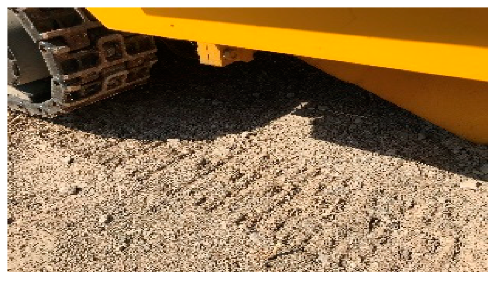
2.1. Road Conditions and Resistance Analysis

The road conditions of a fully mechanized roadway are very complicated [19]. Due to the geological structure and severe working conditions of coal mines, roadheaders are often in a non-horizontal state during the rectification and cutting process [20]. In addition, because of roadway top tray seepage during the excavation process, the roadway floor is typically wet and muddy. Therefore, the track resistance of the roadheader is a highly complicated problem, which includes the compaction resistance, bulldozing resistance, and steering resistance.

2.1.1. Compaction and Bulldozing Resistance

As the floor resistance coefficient cannot be determined, the resistance work estimation method can be used to estimate the track compaction resistance of the roadheader. First, based on the vehicle terramechanics [21], the sinking of the roadheader’s track on the floor can be analyzed:

$$z={(\frac{P}{k_c/b+k_{\phi }})}^{n^{-1}}$$

(1)

In Formula (1), P is the track ground pressure of the roadheader, $k_c$ is the cohesive deformation modulus of the floor, $k_{\phi }$ is the frictional deformation modulus of the road surface, n is the floor subsidence index, and b is the width of the roadheader’s track. Thus, the work of the roadheader’s track to overcome the roadway floor subsidence is:

$$W_F=b{L}_0{{\displaystyle \int }}_0^{z_0}p{d}_z=\frac{b{L}_0}{\left(n+1\right){\left(k_c/b+k_{\phi }\right)}^{n^{-1}}}{p}^{\frac{n+1}{n}}$$

(2)

If the roadheader’s axial displacement in the roadway is $L_0$, the bulldozing resistance is equal to the driving force, so the track driving force work is equal to the bulldozing resistance and is given by $W_{Rz}{=F}_{Rz}{L}_0{=W}_F$. Formula (3), which is the unilateral track bulldozing resistance of the roadheader, can be derived. In this formula, d is the roadheader’s body width, L is the body length, and N is the pressure perpendicular to the roadway floor of the roadheader.

$$F_{Rz}=\frac{b}{\left(n+1\right){\left(k_c/b+k_{\phi }\right)}^{n^{-1}}}{\left(\frac{N}{dL}\right)}^{\frac{n+1}{n}}$$

(3)

In the roadway excavation working face, coal fines are typically found around the roadheader’s track. Thus, the roadheader must overcome the bulldozing resistance caused by these coal fines, as shown in Formula (4). $\gamma$ is the specific gravity of the deposits around the track and $K_c$ and $K_{\gamma }$ are the soil passive coefficients, which can be determined by the road inside friction angle [22].

$$F_{Rb}=\left(0.67cz{K}_c+0.5z^2\gamma K_{\gamma }\right)b$$

(4)

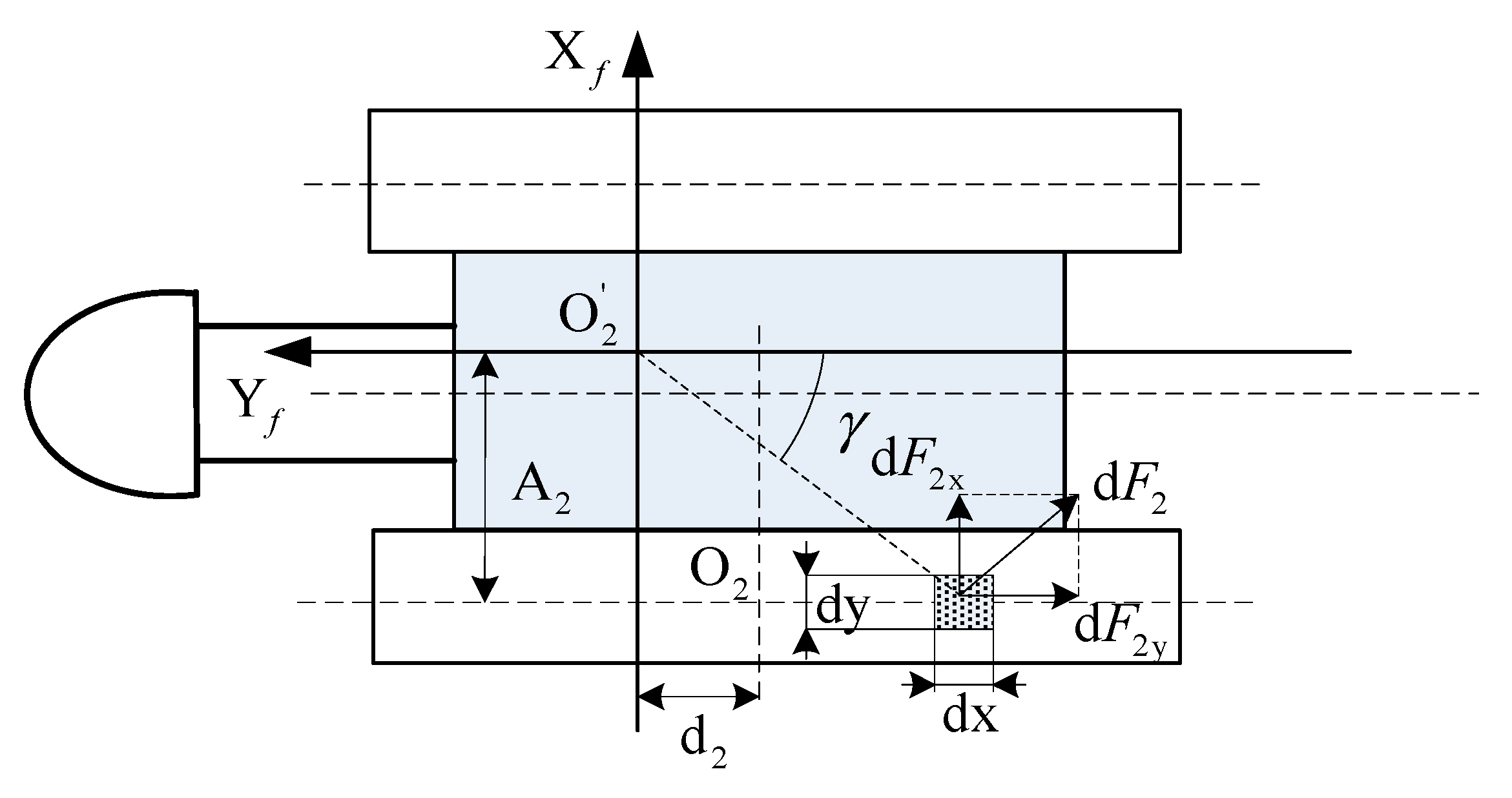
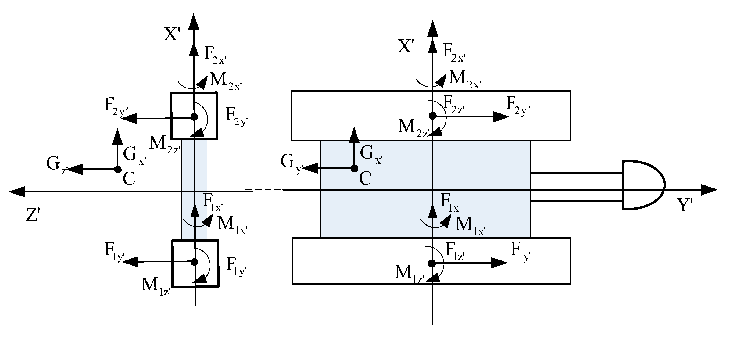
2.1.2. Steering Resistance

The steering resistance between the roadheader’s track and roadway floor is another important component of driving resistance. Taking the roadheader’s right track as an example, the analysis of the resistance during rectification is presented in Figure 1.

A coordinate system was established using the right track instantaneous velocity center as the origin, the roadheader’s excavating direction as the Y axis, and Y’s vertical axis as the X axis. γ is the angle between one point on the track and the instantaneous velocity center, and μ is the roadway floor resistance coefficient. Because there are different forces on different positions of the track, the resistance and moment can be solved by the unit force analysis method. The force at one point on the track is as shown in Formula (5). The floor frictional resistance to the track can be obtained by the integration of Formula (5), which is shown as Formula (6). $d_i$ and $A_i$ are the vertical and lateral offsets of the track instantaneous velocity center on both sides of the roadheader, $b$ is the track width, and $L$ is the track length. The steering resistance moment of the roadway floor can be determined by Formula (7).

$$\{\begin{array}{c}d{F}_{2y}=\mu P_{2}cos\gamma \\ d{F}_{2x}=\mu P_{2}sin\gamma \end{array}$$

(5)

$$\{\begin{array}{c}{F}_{2y}={{\displaystyle \int }}_{-0.5L-d_2}^{0.5L-d_2}\mu P_2\frac{y}{\sqrt{x^2+y^2}}dy{{\displaystyle \int }}_{A_2-0.5b}^{A_2+0.5b}dx\\ F_{2x}={{\displaystyle \int }}_{-0.5L-d_2}^{0.5L-d_2}\mu P_2\frac{x}{\sqrt{x^2+y^2}}dx{{\displaystyle \int }}_{A_2-0.5b}^{A_2+0.5b}dy\end{array}$$

(6)

$$M_{2r}={{\displaystyle \iint }}^{}\left|y+d_2\right|F_{2x}-\left|x-A_2\right|F_{2y}dxdy$$

(7)

The roadheader is one kind of typically slow track vehicle, and the bulldozing resistance of slow track vehicles can be calculated by $F_{Rz}=0.5G\mu$. As a result, the floor resistance coefficient can be calculated inversely through the bulldozing resistance:

$$\mu =\frac{2b}{N\left(n+1\right){\left(k_c/b+k_{\phi }\right)}^{n^{-1}}}{\left(\frac{N}{dL}\right)}^{\frac{n+1}{n}}$$

(8)

Because the lateral resistance on the track from the roadway floor is larger and the rectification speed is very slow, the centripetal force can be ignored. Thus, the slip offset $A_i$ and instantaneous center offset $d_i$ can be regarded as 0. Using Formulas (7) and (8) simultaneously, the roadheader’s rectification resisting moment can be determined.

When the roadheader is running at a small angle, low speed, or uniform speed, the main motion energy consumption is the primary work to overcome the various resistances. Due to the low speed and acceleration in this motion mode, the power consumption of acceleration generation can be ignored in the process of modeling and analyzing the motion system.

According to the above analysis, when driving at a small angle, low speed, or uniform speed, the power consumption of the roadheader satisfies Formula (9):

$$W=\left(F_{Rz}+F_{Rb}\right)dy+0.5Gudy+M_{2r}d\alpha$$

(9)

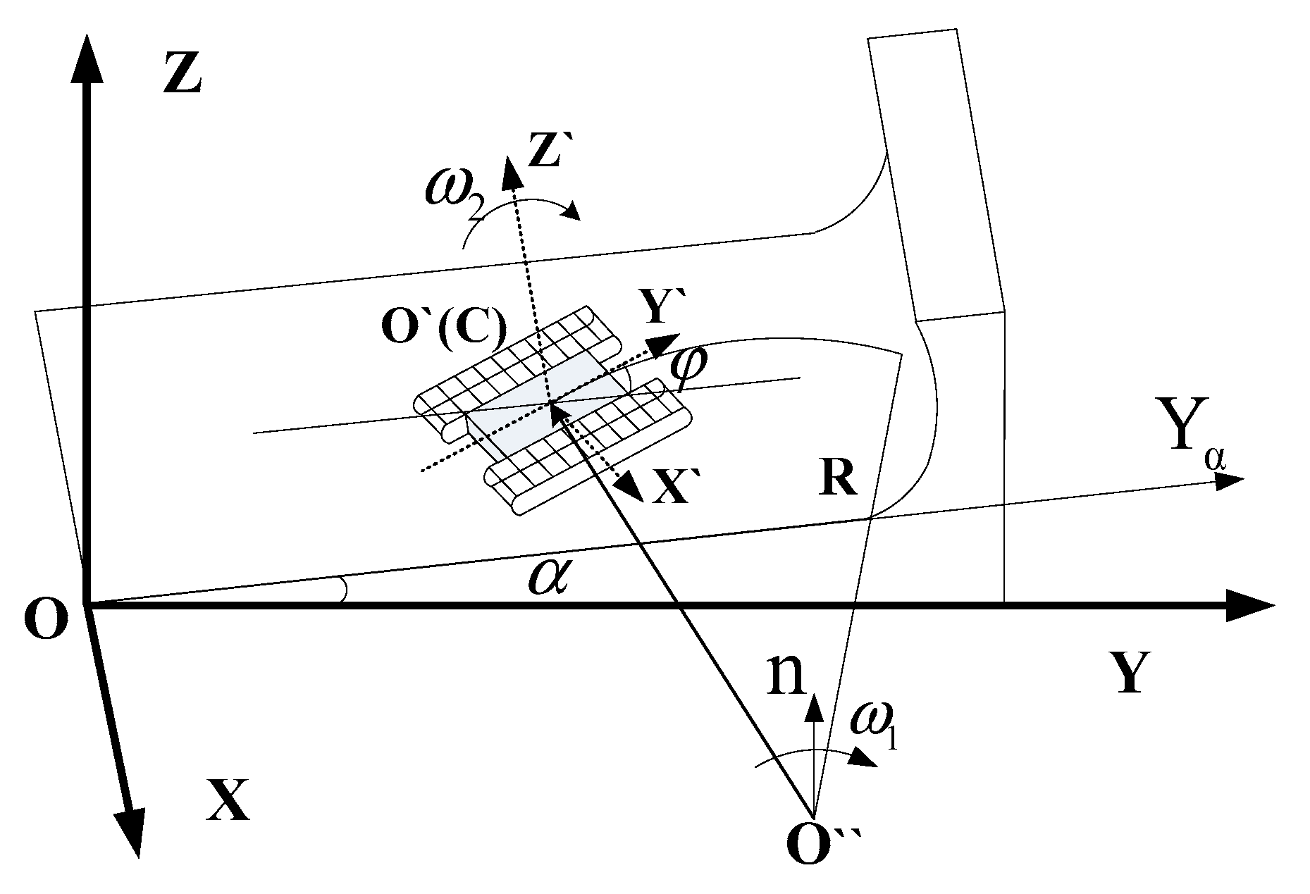
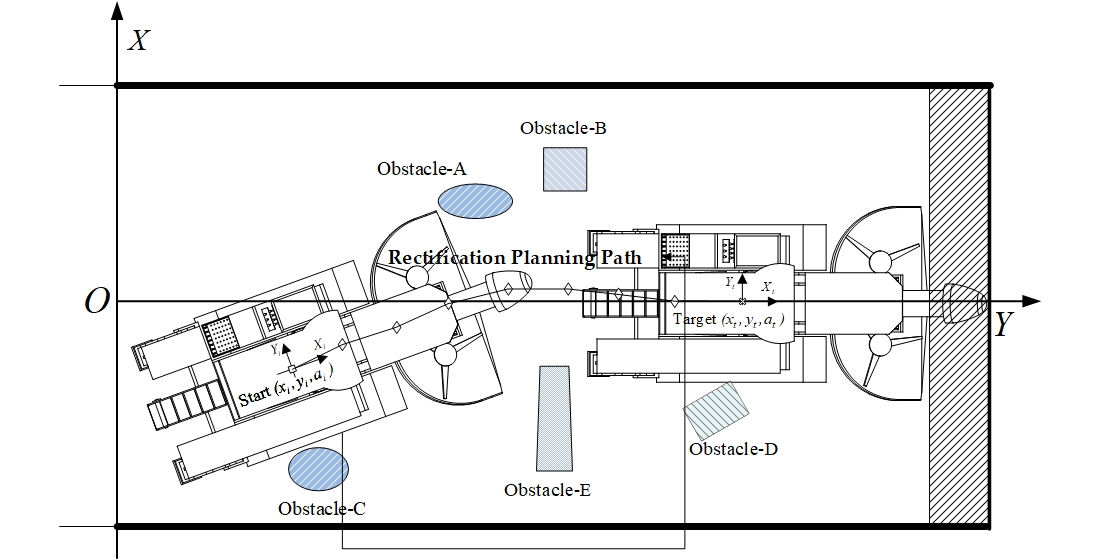
2.2. Kinematic Analysis of Rectifying Machine in a Complex Roadway

In the path planning process of the roadheader—in addition to driving at a small angle, low speed, or uniform speed—further complex working conditions of deviation correction exist, such as: large slope variable speed motion, large angle deviation correction, etc. [20]. In order to build these models of motion, the following analysis of the roadheader’s deviation correction movement in a complex roadway can be made [23,24,25].

The kinematics of the roadheader in the inclined roadway are not in a two-dimensional plane and must be analyzed in three-dimensional space by the space vector method. The roadway coordinate system OXYZ and the roadheader’s frame body coordinate system O’X’Y’Z’ are established in Figure 2. The roadway excavation direction is the Y axis. The inclination angle of the roadway (the angle between the roadway floor and XOY surface) is $\alpha$, which is the most common inclination of the roadway. The rectification motion in the inclined roadway of the roadheader is a composite movement that includes the rotation of the roadheader about the steering center O” and the rotation of the roadheader’s track ground center O’. Ideally, the instantaneous velocity center of the two track sides should coincide with the geometric center of the track. However, considering the actual speed and road conditions of the roadheader, the centrifugal force may be negligible and track slippage could lead to deviation of the instantaneous velocity center from the track’s geometric center.

Taking the inclined roadway floor (face OXYαZ) as the baseline, the model of rectification kinematics of the roadheader is taken from a top-down view. O” is the steering center, L is the track length of the roadheader, B is the center distance of the track, and b is the track width of the roadheader. C is the center of mass of the roadheader, l and d are the lateral and longitudinal offsets of the instantaneous velocity center of the track and the geometric center, respectively, and R is the theoretical turning radius of the roadheader’s rectification.

Suppose that the roadheader only rotates around an axis perpendicular to the ground with no longitudinal pitching motion and yaw, and the roadway inclination has no effect on the driving of the roadheader. The force on the track from the roadway is distributed linearly. During the rectification process, the roadheader’s cutting structure remains still, so the integral structure of the roadheader can be regarded as constant. As a result, the position of the center of gravity of the roadheader $\left[\begin{array}{ccc}{x^{\prime }}_C& {y^{\prime }}_C& {z^{\prime }}_C\end{array}\right]$^T can be determined.

The initial coordinates of the track grounding center O’ are $\left[\begin{array}{ccc}{x}_0& y_0& z_0\end{array}\right]$^T and the vertical vector unit of the roadway coordinate system is [0,0,1]^T. After turning in the inclined roadway, the angle would be ${\left[\begin{array}{ccc}0& -\sin \alpha & \cos \alpha \end{array}\right]}^{\mathrm{T}}$. During rectification of the roadheader, the vertical vector unit rotates in the angle $\phi$. Therefore, the position of the track grounding center in the roadheader’s body coordinate system O’X’Y’Z’ is:

$$n_o^{\prime }=\left[\begin{array}{l}{x}_o\\ y_o\\ z_o\end{array}\right]+\left[\begin{array}{ccc}1& 0& 0\\ 0& \cos \alpha & -\sin \alpha \\ 0& \sin \alpha & \cos \alpha \end{array}\right]\left[\begin{array}{ccc}\cos 0.5\phi & -\sin 0.5\phi & 0\\ \sin 0.5\phi & \cos 0.5\phi & 0\\ 0& 0& 1\end{array}\right]\left[\begin{array}{c}0\\ 2R\sin 0.5\phi \\ 0\end{array}\right]$$

(10)

Thus, the position of the track center in the inclined roadway coordinate system can be obtained by the coordinate transformation of the track grounding center position, and the absolute velocity and acceleration of the roadheader’s centroid can be derived:

$$n_c=\left[\begin{array}{l}{x}_c\\ y_c\\ z_c\end{array}\right]=n_o^{\prime }+\left[\begin{array}{ccc}1& 0& 0\\ 0& \cos \alpha & -\sin \alpha \\ 0& \sin \alpha & \cos \alpha \end{array}\right]\left[\begin{array}{ccc}\cos \phi & -\sin \phi & 0\\ \sin \phi & \cos \phi & 0\\ 0& 0& 1\end{array}\right]\left[\begin{array}{l}{x}_c^{\prime }\\ y_c^{\prime }\\ z_c^{\prime }\end{array}\right]$$

(11)

$$v_c=R_{\phi }\left[\begin{array}{l}-\sin \phi \\ M\\ P\end{array}\right]+\dot{\phi }\left[\begin{array}{l}-x_C^{\prime }\sin \phi -y_C^{\prime }\cos \phi \\ x_C^{\prime }M-y_C^{\prime }Q\\ x_C^{\prime }P-y_C^{\prime }N\end{array}\right]$$

(12)

$$a_c={\ddot{a}}_o+\ddot{\phi }\left[\begin{array}{c}-x_C^{\prime }\sin \phi -y_C^{\prime }\cos \phi \\ x_C^{\prime }M-y^{\prime }Q\\ x_C^{\prime }P-y_C^{\prime }N\end{array}\right]-{\dot{\phi }}^2\left[\begin{array}{c}{x}_C^{\prime }\cos \phi -y_C^{\prime }\sin \phi \\ x_C^{\prime }Q+y_C^{\prime }M\\ x_C^{\prime }N+y_C^{\prime }P\end{array}\right]$$

(13)

Suppose that $M=\cos \alpha \cos \phi$, $N=\sin \alpha \sin \phi$, $P=\sin \alpha \cos \phi$, $Q=\cos \alpha \sin \phi$. When the initial position of the roadheader and the roadway inclination are determined, slippage of the roadheader can be calculated by the methods presented in [14] and [15]. The real centroid velocity and acceleration can be calculated by Formulas (11)–(13).

The dynamic model of the roadheader’s rectification in the inclined roadway needs to establish a dynamic formula in three axes with six degrees of freedom. First, the centroid acceleration of the roadheader’s body can be transformed in the coordinate system O’X’Y’Z’. The vector in the coordinate systems OXYZ and O’X’Y’Z’ can be shown as:

$$a_c^{\prime }=\left[\begin{array}{ccc}\cos \phi & Q& N\\ -\sin \phi & M& P\\ 0& -\sin \alpha & \sin \alpha \end{array}\right]a_c$$

(14)

Limited by the severe conditions in coal mines, the speed and force of the roadheader’s two sides differ during rectification in the roadway. It is assumed that the external forces and moments on the crawlers on the left and right sides in each direction are $F_{i{x}^{\prime }}$, $F_{i{y}^{\prime }}$, $F_{i{z}^{\prime }}$, $M_{i{x}^{\prime }}$, and $M_{i{z}^{\prime }}$, i = 1 or 2. Suppose that all of the external forces on the roadheader track can be simplified to the corresponding side track grounding center, as shown in Figure 3.

$$\{\begin{array}{l}{F}_{1x^{\prime }}+F_{2x^{\prime }}+G_{x^{\prime }}=m{a}_{c{x}^{\prime }}\\ F_{1y^{\prime }}+F_{2y^{\prime }}+G_{y^{\prime }}=m{a}_{c{y}^{\prime }}\\ F_{1z^{\prime }}+F_{2z^{\prime }}+G_{z^{\prime }}=m{a}_{c{z}^{\prime }}\\ M_{1x^{\prime }}+M_{2x^{\prime }}+G_{z^{\prime }}{y}_{c^{\prime }}-G_{y^{\prime }}{z}_{c^{\prime }}=m{a}_{c{z}^{\prime }}{y}_{c^{\prime }}-m{a}_{c{y}^{\prime }}{z}_{c^{\prime }}\\ \left(F_{1z^{\prime }}-F_{2z^{\prime }}\right)0.5B+G_{x^{\prime }}{z}_{c^{\prime }}-G_{z^{\prime }}{x}_{c^{\prime }}=m{a}_{c{z}^{\prime }}{z}_{c^{\prime }}+m{a}_{c{z}^{\prime }}{x}_{c^{\prime }}\\ M_{1z^{\prime }}+M_{2z^{\prime }}+\left(F_{2y^{\prime }}-F_{1y^{\prime }}\right)0.5B+G_{Y^{\prime }}{x}_{c^{\prime }}-G_{x^{\prime }}{y}_{c^{\prime }}=J\ddot{\phi }+m{a}_{c{y}^{\prime }}{x}_{c^{\prime }}-m{a}_{c{x}^{\prime }}{y}_{c^{\prime }}\end{array}$$

(15)

Because the kinematics and structural parameters of the roadheader are already known, $M_{1x^{\prime }}=F_{1z^{\prime }}{L}_{1y^{\prime }}$ and $M_{2x^{\prime }}=F_{2z^{\prime }}{L}_{2y^{\prime }}$, where $L_{1y^{\prime }}$ and $L_{2y^{\prime }}$ are the distance from the equivalent action point of $F_{1z^{\prime }}$ and $F_{2z^{\prime }}$ to the track ground center of the corresponding side track, respectively. Furthermore, $M_{1z^{\prime }}{=-\mu F}_{1z^{\prime }}{L}_{1y^{\prime }}$, $M_{2z^{\prime }}=-{\mu F}_{2z^{\prime }}{L}_{2y^{\prime }}$, and $\mu$ is the steering resistance coefficient of the roadway floor, so the expression of $F_{1z^{\prime }}$ and $F_{2z^{\prime }}$ can be shown as:

$$\{\begin{array}{l}{F}_{1z^{\prime }}=\frac{m{a}_{c{z}^{\prime }}-G_{z^{\prime }}}{2}+\frac{x_{c^{\prime }}\left(G_{z^{\prime }}-m{a}_{c{z}^{\prime }}\right)-z_{c^{\prime }}\left(G_{x^{\prime }}-m{a}_{c{x}^{\prime }}\right)}{B}\\ F_{2z^{\prime }}=\frac{m{a}_{c{z}^{\prime }}-G_{z^{\prime }}}{2}-\frac{x_{c^{\prime }}\left(G_{z^{\prime }}-m{a}_{c{z}^{\prime }}\right)-z_{c^{\prime }}\left(G_{x^{\prime }}-m{a}_{c{x}^{\prime }}\right)}{B}\end{array}$$

(16)

Based on the position of the roadheader’s center of gravity and the inertia force component, combined with the structural characteristics of the walking mechanism of the roadheader, $M_{1x^{\prime }}$ and $M_{2x^{\prime }}$ can be obtained:

$$\{\begin{array}{l}{M}_{1x^{\prime }}=-\left(\frac{B-2x_{c^{\prime }}}{2B}\right)\left[y_{c^{\prime }}\left(G_{z^{\prime }}-m{a}_{c{z}^{\prime }}\right)-z_{c^{\prime }}\left(G_{y^{\prime }}-m{a}_{c{y}^{\prime }}\right)\right]\\ M_{2x^{\prime }}=-\left(\frac{B+2x_{c^{\prime }}}{2B}\right)\left[y_{c^{\prime }}\left(G_{z^{\prime }}-m{a}_{c{z}^{\prime }}\right)-z_{c^{\prime }}\left(G_{y^{\prime }}-m{a}_{c{y}^{\prime }}\right)\right]\end{array}$$

(17)

The positive and negative values of $L_{i\prime }$ correspond to the position of the bottom floor normal equivalent load relative to the position of the track ground center. Given that the track of the roadheader would subside into the roadway, it is accepted that the roadheader’s track is in full contact with the roadway floor. Thus, the resultant force of the unilateral track in x′ and the instantaneous velocity center of the track offset is:

$$\{\begin{array}{l}{F}_{i{x}^{\prime }}=\frac{F_{i{z}^{\prime }}}{L}\left(3L_{i{y}^{\prime }}-2d_i-\frac{12L_{i{y}^{\prime }}}{L^2}{d}_i{}^2\right)\\ d_i=\frac{-Y\pm \overline{Y^2-4XZ}}{2X}\end{array}$$

(18)

In Formula (18), suppose that ${X=12(M}_{1x^{\prime }}{+M}_{2x^{\prime }}{)/L, Y=2(F}_{1z^{\prime }}{+F}_{2z^{\prime }})/L$, and $Z=-3\left(M_{1x^{\prime }}{+M}_{2x^{\prime }}\right){-(G}_{x\prime }{-ma}_{c{x}^{\prime }})/L$. $d_i$ can be determined by the structure and motion parameters of the roadheader. Then, $F_{i{x}^{\prime }}$ and other parameters,$M_i=M_{i{z}^{\prime }}+d_i{F}_{i{x}^{\prime }}$ and $M_r=M_1+M_2$, can be obtained:

$$M_{i{z}^{\prime }}={\displaystyle \int \begin{array}{l}{d}_i\\ -0.5L\end{array}}\mu P_{i{y}^{\prime }}b\left(y^{\prime }-d_i\right)d{y}^{\prime }-{\displaystyle \int \begin{array}{l}0.5L\\ d_i\end{array}}\mu P_{i{y}^{\prime }}b\left(y^{\prime }-d_i\right)d{y}^{\prime }-d_i{F}_{i{x}^{\prime }}$$

(19)

According to the above analysis, the driving force on both sides of the roadheader can be calculated by the simultaneous formulas including the y′ motion and the rotation around z′. The expression of the driving force on both sides of the roadheader are shown in Formula (20):

$$\{\begin{array}{l}{F}_{1y^{\prime }}=-0.5Y+(M_{1z^{\prime }}+M_{2z^{\prime }}+x_{c^{\prime }}Y-y_{c^{\prime }}X-y_{c^{\prime }}Z)/B\\ F_{2y^{\prime }}=-0.5Y-(M_{1z^{\prime }}+M_{2z^{\prime }}+x_{c^{\prime }}Y-y_{c^{\prime }}X-y_{c^{\prime }}Z)/B\end{array}$$

(20)

The above theory provides a theoretical basis for the dynamic analysis of roadheaders operating under complex working conditions; that is, the relevant energy consumption calculation. Through the above analysis, it can be concluded that the energy consumption formula of a roadheader under complex working conditions is:

$$W=\left(F_{1x^{\prime }}+F_{2x^{\prime }}\right)dx+\left(F_{1y^{\prime }}+F_{2y^{\prime }}\right)dy+\left(F_{1z^{\prime }}+F_{2z^{\prime }}\right)dz+\left(M_{1z^{\prime }}+M_{2z^{\prime }}\right)d\alpha +\left(M_{1x^{\prime }}+M_{1x^{\prime }}\right)d\phi +\left(M_{1y^{\prime }}+M_{1y^{\prime }}\right)d\beta$$

(21)

where $\beta$ is the roll angle, $\phi$ is the pitch angle, and $\alpha$ is the march angle.

2.3. Driving Performance Analysis of the Roadheader

In order to ensure the reliability of the roadheader auto-rectification control and the correct planning of the best rectifying path, the driving performance of the roadheader needed to be analyzed, including its ability to cross trenches and vertical obstacles. This performance is mainly affected by its motion performance and mechanism geometry. The parameters are also related to the inclination of the roadway and the physical parameters of the ground surface [26,27].

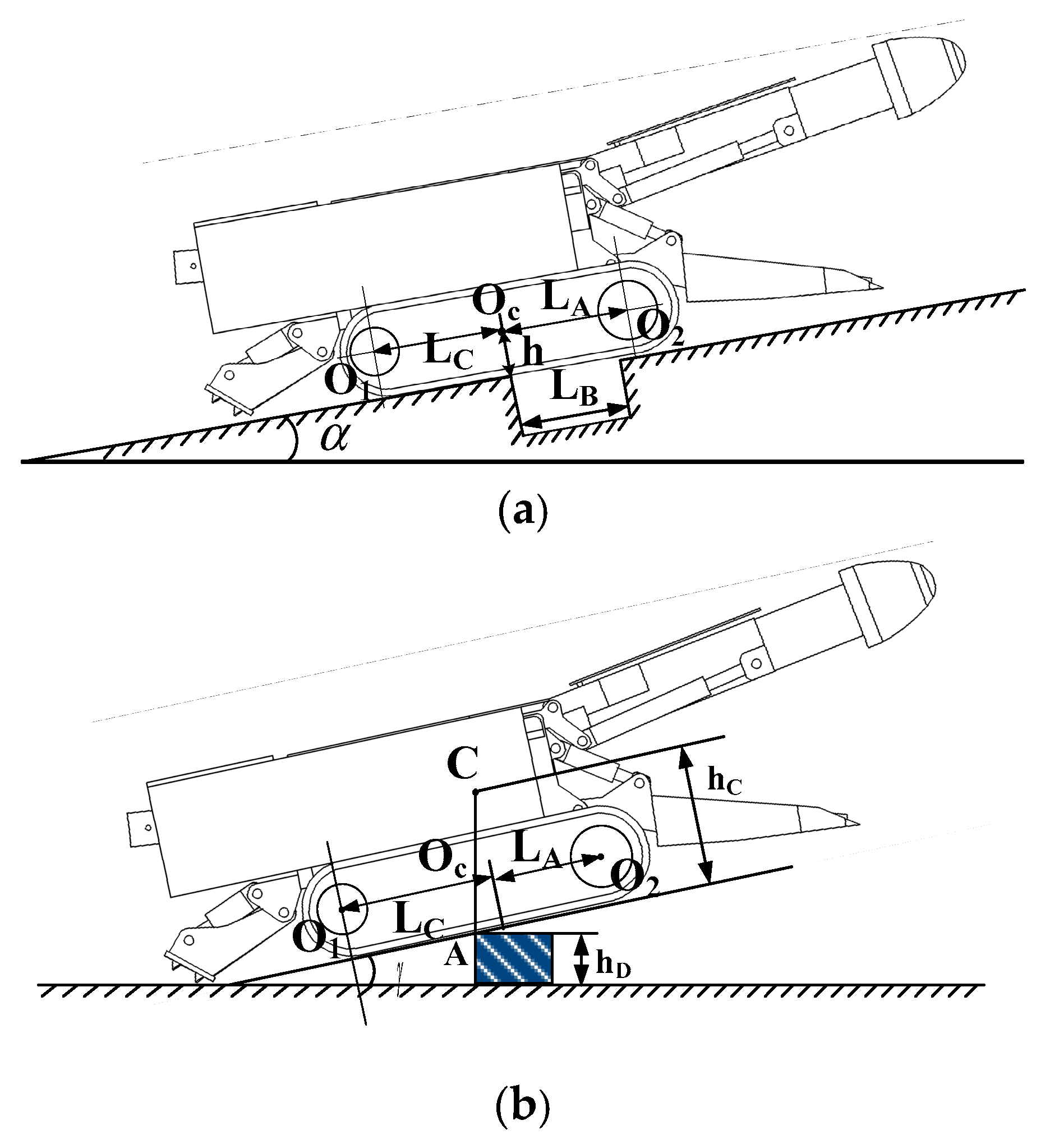
2.3.1. Trench-Crossing Capability of the Roadheader

The trench-crossing capacity of the roadheader on an inclined roadway, as shown in Figure 2, was analyzed. The slope of the roadway is described by the following: $\alpha$ is the roadway’s inclination angle and h is the distance between the roadheader’s centroid and roadway floor. The support points at both ends of the track are the track drive wheel center O₁ and the guide wheel center O₂ of the roadheader. The width of the trench in the roadway that the roadheader should cross is L_B. L_C is the horizontal distance between the driving wheel center and the roadheader’s centroid. L_A is the horizontal distance between the guiding wheel center and the roadheader’s centroid.

When the roadheader crosses a trench, the roadheader’s centroid often remains behind the trench so as to prevent it falling in [28]. When the front of the roadheader crosses the trench, because the centroid of the roadheader leans back, it falls more easily on inclined roadways than on even roadways.

At this time, the maximum trench-cross width of the roadheader is the minimum value between $L_B{=L}_A- h \tan \alpha$ and $L_B{=L}_C+h \tan \alpha$. If the roadway is inclined downward, the analysis method is similar, and the maximum trench-cross width is the minimum width between $L_B{=L}_C- h \tan \alpha$ and $L_B{=L}_A+h \tan \alpha$.

2.3.2. Analysis of Obstacle-Crossing Capability of the Roadheader

The limit state of the roadheader’s obstacle-crossing capability is shown in the bottom of Figure 4. C is the roadheader’s centroid, h_c is the distance from the centroid to the bottom of the track, h_D is the height of the obstacle, and $\gamma$ is the angle between the roadheader’s chassis and the roadway floor. When the roadheader’s track front part A touches the obstacle, the front part of the roadheader moves vertically upward along the obstacle, thereby causing a clockwise rotation motion. The centroid rises and the angle between the chassis and the floor continues to increase. The roadheader’s centroid being completely on top of the obstacle is the limiting condition of the roadheader crossing the vertical obstacle. After the crossing, the roadheader continues to move normally in the roadway. The calculation method of the vertical obstacle height is shown in Formula (22):

$$\{\begin{array}{l}{h}_d=L_c\sin \gamma -h_c\cos \gamma \\ \sin \gamma =\frac{h_d}{L_C+L_A}\\ \cos \gamma =(\sqrt{(L_c+L_A{)}^2-h_d^2})/(L_c+L_A)\end{array}$$

(22)

According to Formula (22), the maximum obstacle height that the roadheader can cross in a horizontal roadway is only related to the roadheader structural parameters $L_c$, $L_A$, and $h_c$. The position of the roadheader centroid can be shifted by an inclined roadway, and the maximum vertical obstacle height for an inclined roadway can be obtained by $L_{c^{\prime }}$, $L_{A^{\prime }}$, and $h_{c^{\prime }}$.

$$\{\begin{array}{l}{L}_{C^{\prime }}=L_C-h\tan \alpha \left(-90°<\alpha <90°\right)\\ L_{A^{\prime }}=L_A+h\tan \alpha \left(-90°<\alpha <90°\right)\\ h_{C^{\prime }}=h_C\end{array}$$

(23)

The above theory provides the calculation basis for estimating the ability of roadheaders to cross over trenches and obstacles in roadways.

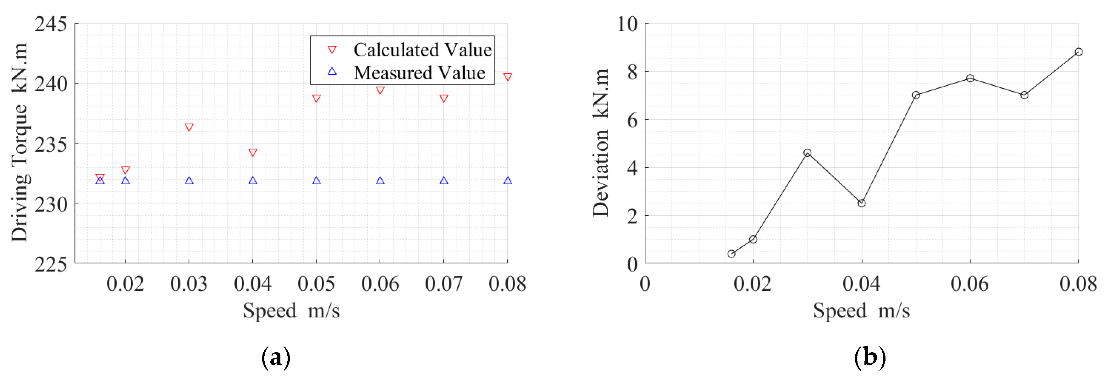
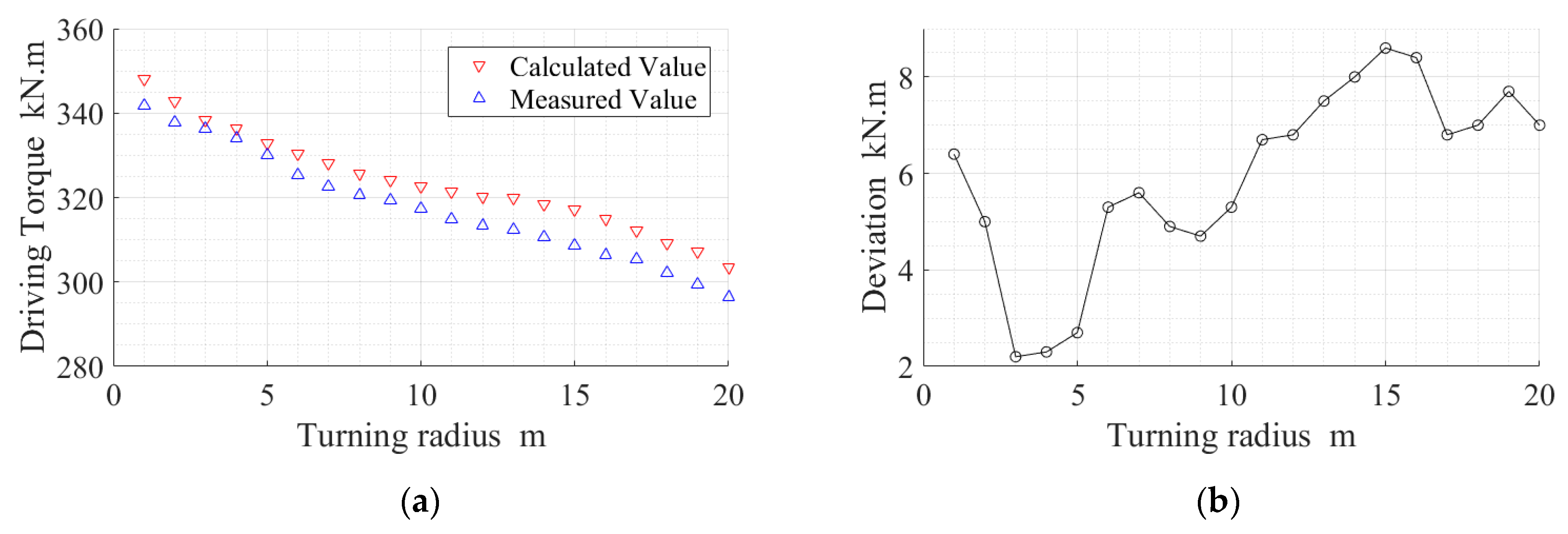
2.4. Experimental Verification

In order to verify the rectification kinematic and dynamic models of the roadheader on an inclined roadway [2], the EBZ-55 roadheader was taken as an experimental example. Experiments regarding uniform motion in a straight line on horizontal ground (Figure 5) and turning motion on a slope (Figure 6) were carried out. The uniform motion in a straight line experiment (Figure 5) was conducted on an experimental roadway which was 4 m wide and 25 m long. The experimental ground was cement ground with a rectangular roadway, which was not suitable for large angle turning, but was suitable for a uniform linear motion test. The turning motion on a slope experiment (Figure 6) was conducted on sandy soil with an inclination angle of 3.475° from the floor. During the experiment, the roadheader moved at the speed of 0.05 m/s and also turned at about 0.05 m/s. The experimental site in Figure 6 was built with sandy soil and had a certain inclination angle, which could meet the various turning movements of the roadheader.

In the experiment, rotational speed was measured using a photoelectric sensor. The torque was measured using a torque sensor. The steering angle and speed could be measured in real time using an automatic laser overall meter and laser distance meter. All experimental data were collected by the NI data acquisition card and stored on the onboard PLC control system of the roadheader. All of the data collected in the PLC control system were later sent to the upper computer via Ethernet [29]. The experimental data of uniform motion are presented in Figure 7, Figure 7a shows the relationship between measured torque and calculated torque with running speed, and Figure 7b shows the relationship between the deviation between measured torque and calculated torque with running speed. The comparison between the data calculated by the methods in Section 2.1 and the experimental data are presented in

Table 1. Comparison between experimental and calculated data of uniform motion.

Parameter	Measuring Point of Maximum Driving Torque		Measuring Point of Maximum Deviation
	Driving Torque (KN·m)	Speed (m/s)	Driving Torque (KN·m)	Speed (m/s)
Calculated value	231.8150	0.08	231.8150	0.08
Measured value	241.2238	0.0786	241.2238	0.0786
Deviation	9.6088	0.0014	9.6088	0.0014

.

According to Figure 7, it can be concluded that the maximum deviation point of the measured value and calculated value and the maximum driving torque point of the measured value are the moving points of the roadheader at the speed of 0.08m/s during the straight-line walking process. As shown in Table 1.

The experimental data of turning motion on a slope are presented in Figure 8, and a comparison between the data calculated by the methods in Section 2.2 and the experimental data are presented in

Table 2. Comparison between experimental and calculated data of turning motion on slope.

Parameter	Measuring Point of Maximum Driving Torque		Measuring Point of Maximum Deviation
	Driving Torque (KN·m)	Radius (m)	Driving Torque (KN·m)	Radius (m)
Calculated value	341.659	1	308.544	15
Measured value	348.324	1.08	317.268	15.42
Deviation	7.57	0.08	8.72	0.42

. Figure 8a shows the relationship between measured torque and calculated torque with turning radius, and Figure 8b shows the relationship between the deviation between measured torque and calculated torque and the turning radius. A hydraulic motor was required to maintain approximately uniform and stable motion throughout the experiment.

Figure 8 shows that in the process of the roadheader’s turning motion on a slope, the maximum deviation point between measured value and calculated value is the test point with a turning radius of 15 m, and the maximum driving torque point measured value is the test point with a turning radius of 1 m, as shown in Table 2.

According to the experimental results, the maximum error between the calculated values of the theoretical model and the experimental values did not exceed 5%, which indicated that the calculated results were close to the actual measured results. As a result, the accuracy of the model proposed in Section 2.1 and Section 2.2 could be verified.

3. Automatic Rectification Planning Algorithm for the Roadheader

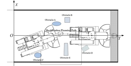
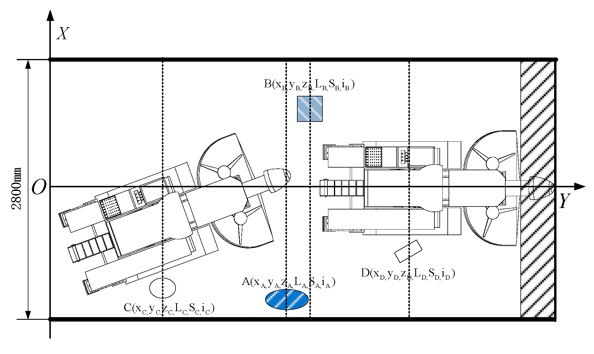
3.1. Roadway Environment Modeling

The grid environment model is the traditional method to describe obstacle information in a two-dimensional environment in a robot’s path. The working space of the roadheader is a sloped comprehensive roadway with closed boundaries. There are a variety of influential factors on the roadway floor that affect the rectification of the roadheader. The roadheader has strong environmental adaptability to navigate the numerous different road conditions encountered on the roadway floor. Therefore, it is necessary to combine the information relating to the road surface parameters, inclination, roadheader’s driving performance, and obstacles in the model. Because the rectification of the roadheader is not directly related to the height of the roadway, the model established here is a two-dimensional (2D) environment model. The Y axis is the roadway excavation direction and the X axis is perpendicular to OY. The two-dimensional (2D) roadway coordinate system can then be established, which is presented in Figure 9.

Taking area A in Figure 9 as an example: it can be regarded as a dataset of six-dimensional attributes $\left\{N_i=\left(x_i{,y}_i{,z}_i{,L}_i{,S}_i,i\right),i=1,2,\cdots ,n\right\}. x_A$ and $y_A$ are the coordinates of the center position of one road area, which can be regarded as the position attributes. $z_A$ is the maximum height or depth of the road area, which is an elevation attribute. $L_i$ is the trench width of the road area, which is the width attribute. $S_A$ is the projected area of the road area, which is the area attribute. $i_A$ is the slip rate of the road conditions ($i_A{=1-\mu }_A{/\mu }_{\max }$) and is the pass attribute.

Some perpendiculars can be obtained by the road projection area center point and Y axis. Therefore, the clusters of parallel lines $\left\{L_1{L}_2\cdots L_n\right\}$ can be determined. n is the number of unconventional road conditions areas in the restricted roadway space. With the previous attributes determined, the environment modeling of the roadway space is completed.

3.2. Rectification Impact Degree (RID) of the Roadheader

As a large number of unconventional road conditions exist in the roadway that need to be marked, and as they exert different influences on the optimal rectification strategy and control, the concept of autonomous rectification influence degree of the roadheader is proposed in regard to the driving performance of the roadheader and its working conditions [29]. The influence degree of rectification primarily consists of two parts: the rectification impact degree (RID) and the rectification cost (RC) of the roadheader.

3.2.1. Automatic Rectification Impact Degree (RID) of the Roadheader

$$I={\omega }_1\frac{x_{\max }-x_n}{x_{\max }}+{\omega }_2\frac{z_n}{z_{\max }}+{\omega }_3\frac{L_{Bn}}{L_{B\max }}+{\omega }_4\frac{S_n}{S_{\max }}+{\omega }_5\frac{i_n}{1-i_{\min }}$$

(24)

In Formula (24), $x_n$ and $z_n$ are the coordinates of the unconventional road condition center. $x_{\max }$ and ${ z}_{\max }$ are the maximum of the coordinates and height of the center point of all road conditions. $L_{Bn}$ and ${ L}_{B\max }$ are the trench width and the widest of the depression trench widths, respectively. $S_n$ and $S_{\max }$ are the single road area and maximum of all projection areas, respectively. $i_n$ and $i_{\min }$ are the slip rate in a certain area and the minimum slip rate in all unconventional road condition areas, respectively. $\omega$ is the weight corresponding to each attribute, and ${\omega }_1{+\omega }_2{+\omega }_3{+\omega }_4{+\omega }_5=1$. When determining the rectification weight of each area, each area can only have vertical obstacles or depressions, so when $z_n>0$, then ${\omega }_3=0$. Conversely, if $z_n<0$, then ${\omega }_2=0$. Other weights are allocated based on the driving conditions of the roadheader and actual experience.

$${\omega }_i=\{\begin{array}{l}\left[0.15,0.35,0,0.1,0.3\right]\left(z_n>0\right)\\ \left[0.15,0,0.35,0.1,0.3\right]\left(z_n<0\right)\end{array}$$

(25)

3.2.2. Simplified Roadway Grid Model

In the process of the roadheader’s path rectification planning, the greater number of 2D roadway environment rasters used, the more time needed for calculations [30,31,32]. Therefore, it is necessary to simplify the grid model through the calculation results of the obstacle-surmounting ability presented in Section 2.3.

All non-conventional road conditions areas are known in the roadway model. The deletion of the road conditions areas with less influence on the rectification can simplify the model and reduce the time required to solve the dimension. $[x_{t1}{,x}_{t2}]$ is the position interval, $[z_{t1}{,z}_{t2}]$ is the elevation interval, $\left[L_{Bt1},L_{Bt2}\right]$ is the width interval, [$S_{t1}{,S}_{t2}]$ is the area interval, and [$i_{t1},i_{t2}]$ is the road passing interval. The regional grid retention and deletion principles are as follows:

• When $x_n$ is less than the minimum $x_{t1}$ and other values are within the value range, this grid must be reserved and marked as an impassable area.
• When $z_n$ and $L_{Bn}$ are greater than their maximum values $z_{t2}$ and $L_{Bt2}$, this grid must be retained as a passable area.
• When $i_n$ is greater than the maximum $i_{t2}$ and other values are within its value range, this grid must be retained and the area cannot be traversed.
• In addition to the above, a threshold value $I_t$ is proposed. When the rectification influence degree is greater than this threshold, the grid should be reserved or otherwise deleted.

3.2.3. Rectification Cost (RC) of the Roadheader

The RC of a roadheader can be regarded as the reference information for selecting the best path. The calculation expression is as shown in Formula (26): T is the total cost of the roadheader’s rectification process, $I_1$ is the influence degree of rectification when passing the unconventional road area, $D_1$ is the distance from the center of the road area to the path trajectory point, and ${D^{\prime }}_1$ is the distance from the center of the track near the roadheader to the road area center.

$${T=I}_1\frac{D_1^{\prime }}{D_1}+\cdots {+I}_n\frac{D_n^{\prime }}{D_n} (I \mathrm{is} \mathrm{only} \mathrm{accessible} \mathrm{area})$$

(26)

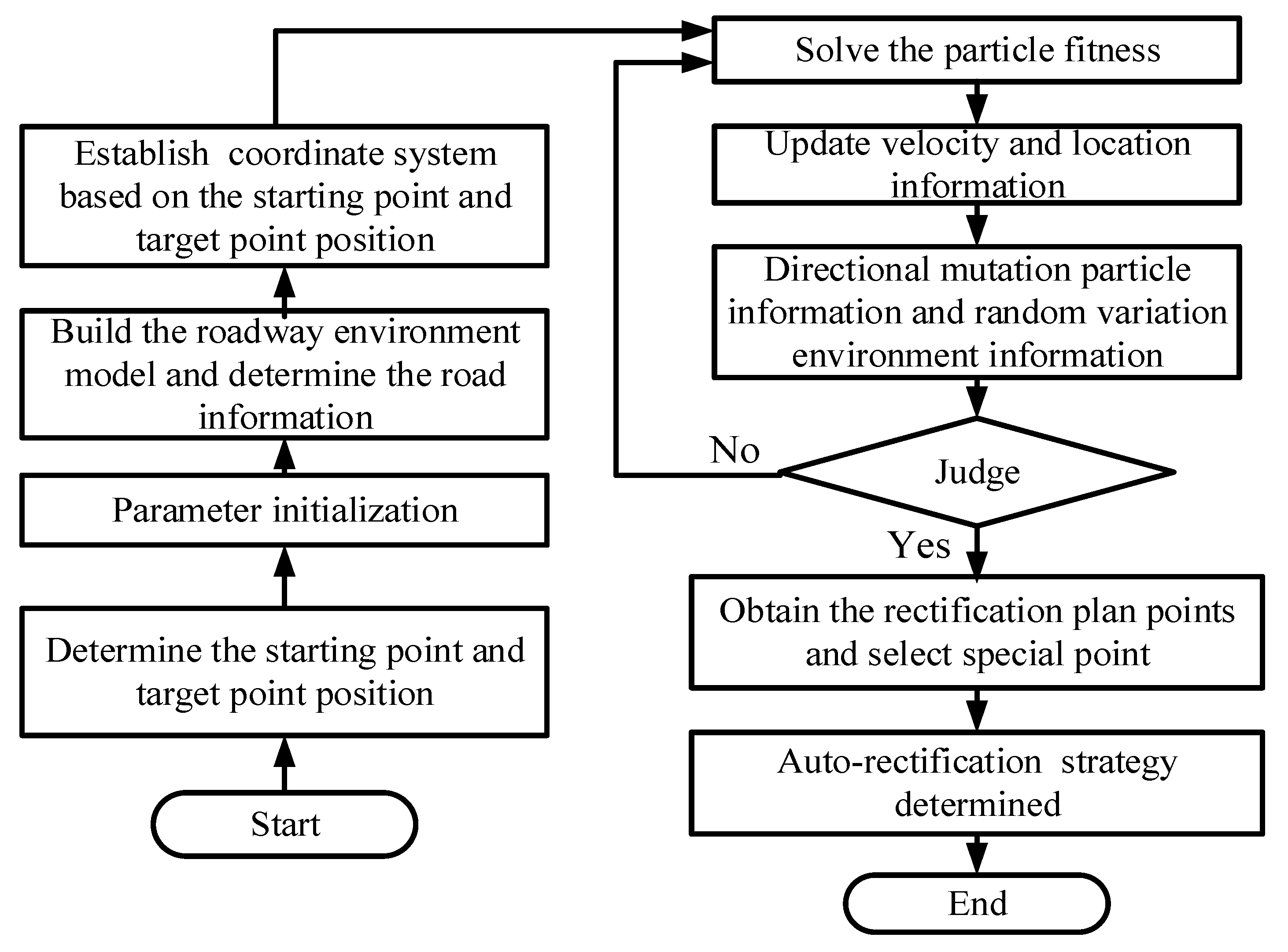
3.3. Rectification Plan Algorithm for the Roadheader

The automatic rectification of the roadheader in the roadway refers to moving and purposefully steering in the narrow and confined space, based on the known roadway size, road conditions, and obstacles. First of all, in the single rectification travel distance of the roadheader, the rectification path plan is based on the structure, the driving characteristics of the roadheader, and the actual road conditions. Then, the key points of the rectification path plan can be obtained. Based on these path plan key points and the path trajectory and kinematic characteristics of the roadheader, the roadheader can track the rectification points in this area so as to achieve various rectification transfer strategies.

3.3.1. Mutation Particle Swarm Optimization Rectification Algorithm (PSO) for the Roadheader

The particle swarm algorithm specifies the behavior rules of particles without mass and volume to reveal certain behavior characteristics. The particles in the target optimization continuously search in a D-dimensional space [33,34,35]. Suppose that the roadheader initial point coordinate in the roadway environment model roadheader is ${(x}_0{,y}_0)$, the target point coordinates are $\left(x_g{,y}_g\right)$, the initial deflection angle of the roadheader is ${\alpha }_0$, and the target deflection angle is ${\alpha }_g$. The single deflection angle of the roadheader $\Delta {\alpha }_t$ and path S are given by:

$$\Delta {\alpha }_t=\arctan \left|\frac{\frac{y_{j+1}-y_j}{x_{j+1}-x_j}-\frac{y_j-y_{j-1}}{x_j-x_{j-1}}}{1+\frac{y_j-y_{j-1}}{x_j-x_{j-1}}\times \frac{y_{j+1}-y_j}{x_{j+1}-x_j}}\right|$$

(27)

$$S={\Sigma }_{j=0}^n\sqrt{{\left(x_j-x_{j+1}\right)}^2+{\left(y_j-y_{j+1}\right)}^2}$$

(28)

The closest distance between the path point and the center point of the impassable area or the roadway boundary is used as the rectification safety index (RSI). $D_{di}$ in Formula (29) is the roadheader’s rectification safety index regarding the ith impassable area and $x_{di}$ and $y_{di}$ are the coordinates of the center point of the ith impassable area.

$$D_{di}={\Sigma }_{j=0}^n\sqrt{{\left(x_j-x_{di}\right)}^2+{\left(y_j-y_{di}\right)}^2}$$

(29)

At the same time, in the expected path planning process, the energy consumption should be as small as possible to ensure that the roadheader avoids overloading during long periods of operation. Therefore, the parameter energy consumption index (ECI) is proposed. $W_{di}$ is the ECI parameter of the roadheader, when it passes the ith zone.

$$W_{di}={\displaystyle {\sum }_{j=0}^n{W}_j}$$

(30)

According to the dynamic model analysis results of roadheaders presented in Section 2, the movement process of the roadheader in the jth path planning process of the ith area can be divided into two states according to the rectification angle:

• When the rectification angle is smaller than 5°, the ECI of the roadheader is calculated according to the motion model in Section 2.1. Therefore, $W_j$ is calculated according to Formula (9): $W_j=\left(F_{Rz}+F_{Rb}\right)\left(y_j-y_{di}\right)+0.5Gu\left(y_j-y_{di}\right)+M_{2r}\left({\alpha }_j-{\alpha }_{di}\right)$.
• When the rectification angle is large or operating at variable speed is required, the ECI of the roadheader is calculated according to the motion model in Section 2.2. Therefore, $W_j$ is calculated according to Formula (21). The grid model in Section 3.2 does not take into account the change of pitch angle and roll angle during the operation of the roadheader:

  $$W_j=\left(F_{1x^{\prime }}+F_{2x^{\prime }}\right)\left(x_j-x_{di}\right)+\left(F_{1y^{\prime }}+F_{2y^{\prime }}\right)\left(y_j-y_{di}\right)+\left(M_{1z^{\prime }}+M_{2z^{\prime }}\right)\left({\alpha }_j-{\alpha }_{di}\right)$$

Because there are many constraints in the roadheader’s rectification planning, a rectification cost threshold P based on the roadheader’s rectification influence degree and coincident area can be set. All rectification plan situations can be divided into three categories:

• The first category is in the safe area and the cost is less than the rectification cost threshold P.
• The second category is passing a non-traversable area.
• The third category is a safe area but the cost is greater than the threshold.

According to the above analysis, a penalty function was used to transform the path rectification planning into an unconstrained optimization problem, and the individual fitness was adjusted at the same time.

$$F=\{\begin{array}{l}\varphi \left(x,y,\alpha \right)={\epsilon }_{1}S+{\epsilon }_2{D}_d{}_i+{\epsilon }_3{W}_{di},{{\displaystyle }}_{}{{\displaystyle }}_{}{{\displaystyle }}_{}{{\displaystyle }}_{}\hspace{1em}\mathrm{the} \mathrm{first} \mathrm{category}\\ \varphi \left(x,y,\alpha \right)={\epsilon }_{1}S+{\epsilon }_2{D}_d{}_i+{\epsilon }_3{W}_{di}+U_1,{{\displaystyle }}_{}\hspace{1em}\mathrm{the} \mathrm{second} \mathrm{category}\\ \varphi \left(x,y,\alpha \right)={\epsilon }_{1}S+{\epsilon }_2{D}_d{}_i+{\epsilon }_3{W}_{di}+U_2,{{\displaystyle }}_{}{{\displaystyle }}_{}\hspace{1em}\mathrm{the} \mathrm{third} \mathrm{category}\end{array}$$

(31)

In Formula (31), ${\epsilon }_1+{\epsilon }_2+{\epsilon }_3=1$, $\epsilon =\left\{{\epsilon }_1,{\epsilon }_2,{\epsilon }_3\right\}$ is set according to the analyst’s emphasis on path distance S, RSI, and ECI.

In the standard particle swarm optimization algorithm, the particle position in each dimension corresponds to each straight line in the roadway environment model. The particle position coordinates $x_{i,j}$ and $y_{i,j}$ of each dimension correspond to the ordinate $x_{i,j}$ and abscissa $y_{i,j}$ of the optimal solution $p_j$; that is, the best path point and the best target deflection angle in the rectification. Because the particle swarm would approach the local minimum infinitely, the optimal value of the objective function cannot be solved [36]. This paper proposes a multidimensional mutation-adaptive particle swarm algorithm based on the roadheader influence degree. The solution distributed in the vertical direction of the fully mechanized excavation roadway can be shrunk directionally. The concept of mutation operator, which includes directional mutation and random mutation, was also investigated. The directional mutation is always used to update and reset the particle information obtained after iteration, and its variation approaches are:

$$\begin{array}{l}{m}_{i,j}=\{\begin{array}{l}\frac{(x_{i,j-1}+x_{i,j+1})}{2}, rand(1)\ge p_1\\ 0, rand(1)<p_1\end{array}\\ n_{i,j}=\{\begin{array}{l}{x}_{\max }\times rand(1,M), rand(1)\ge p_2\\ x_{i,j}, rand(1)<p_2\end{array}\end{array}$$

(32)

In Formula (32)${, m}_{i,j}$ is the directional mutation operator, which is used to update and reset particle information obtained after an iteration, and $n_{i,j}$ is the random mutation operator used to update the waypoints in the roadheader’s driving direction in the roadway model. Substituting the two-particle information into the directional mutation formula, we obtain the changed value. $p_1$ is the directional mutation threshold, $p_1\in (0,1)$, and $x_{\max }$ is the maximum particle position within the allowable range.

3.3.2. Marking and Tracking of the Roadheader’s Rectification Points

Through this algorithm, the rectification plan points of the roadheader can be obtained. Because the road conditions of the comprehensive roadway are complicated and the roadheader’s adaptability to road conditions is strong, the key points can be marked in all the trajectory points on the basis of the rectification trajectory points, and the roadheader can overcome traffic conditions and move between the key position points [37]. However, the motion of the roadheader could be set as only four modes—such as straight travel and pivot steering—thereby simplifying the complexity and thus reducing the adjustment times in the process of roadheader rectification. The overall process is presented in Figure 10.

(1) Points find and select

The initial point coordinates of the roadheader are ${(x}_0{,y}_0{,\alpha }_0)$, the target point coordinates are ${(x}_g{,y}_g{,\alpha }_g)$, and the track point is ${(x}_i{,y}_i{,\alpha }_i)$. A is forward motion, B is backward motion, C is anticlockwise pivot steering, and D is clockwise pivot steering. Start by searching from the first track point. When ${\alpha }_i\cong {\alpha }_0$, determine whether the roadheader could pass on the line track between the two points. If passable, when $y_i>y_0$, mark this track point as class A, and if $y_i<y_0$, it can be classified as class B. If no such track point appears, restart the search. When ${ x}_i\cong x_0$ and $y_i\cong y_0$, if ${\alpha }_i>{\alpha }_0$, mark this track point as class C. If ${\alpha }_i<{\alpha }_0$, mark this track point as class D.

(2) Points make and track

Here, we take the A-C-A-D point-finding process as an example to describe the point-making and tracking process. The roadheader moves straight from the initial point to the first point of class A. Then, the first point is updated to point 0’, and it turns to the second point of class C, which is updated to point 0’’ before the roadheader moves straight to the third point of class A. This third point can be updated to point 0’’’ upon arrival, and the roadheader turns to the fourth point of class D to complete the whole process.

During this process, the roadheader only made four moves, which greatly simplified the rectification process. Based on the point in the optimal rectification plan, the driving performance of the roadheader can be used to its maximum extent, which further improves the efficiency and accuracy of the roadheader’s auto-rectification in the fully mechanized excavation roadway.

4. Simulation and Experiment of the Roadheader’s Rectification Plan

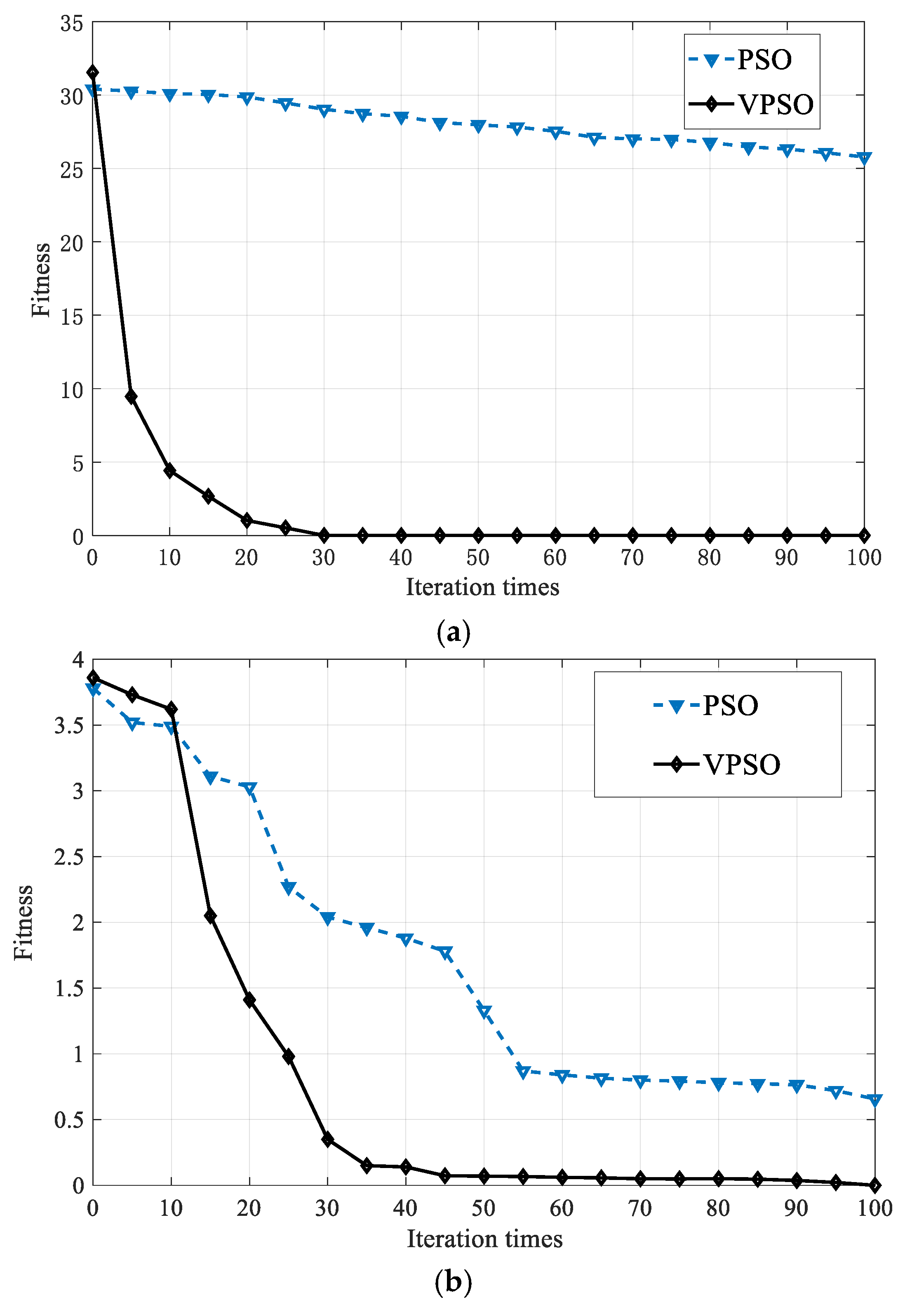
4.1. Rectification Plan Algorithm Simulation

4.1.1. The Simulation of the Roadheader’s Rectification Plan Algorithm

In the simulation of the roadheader’s rectification plan algorithm, the particle swarm size was N = 40, the maximum searching speed was $v_{\max }=1$, the inertia weight interval was (0.4165, 0.8298), the learning factor was $c_1{=c}_2=1.4962$, the number of iterations was 100, and the variation threshold was 0.99. There are two kinds of unconstrained optimization functions, Ackley (A function) and Griewank (G function) [38]. They can be used as test functions to compare the performance of the mutation particle swarm rectification plan algorithm and the standard particle swarm algorithm. The results following 20 simulations are presented in Figure 11 and

Table 3. The minimum fitness of the two algorithms.

Algorithm	A Function		G Function
	Average Iterations	Minimum Fitness	Average Iterations	Minimum Fitness
PSO	100		57.6	10
VPSO	28.4	2 × 10−7	35.6	0.0047

.

Although the two kinds of particle swarm optimization can both quickly search the minimum fitness and maintain good precision and stability, the VPSO algorithm is much better than the PSO algorithm in terms of search speed and accuracy.

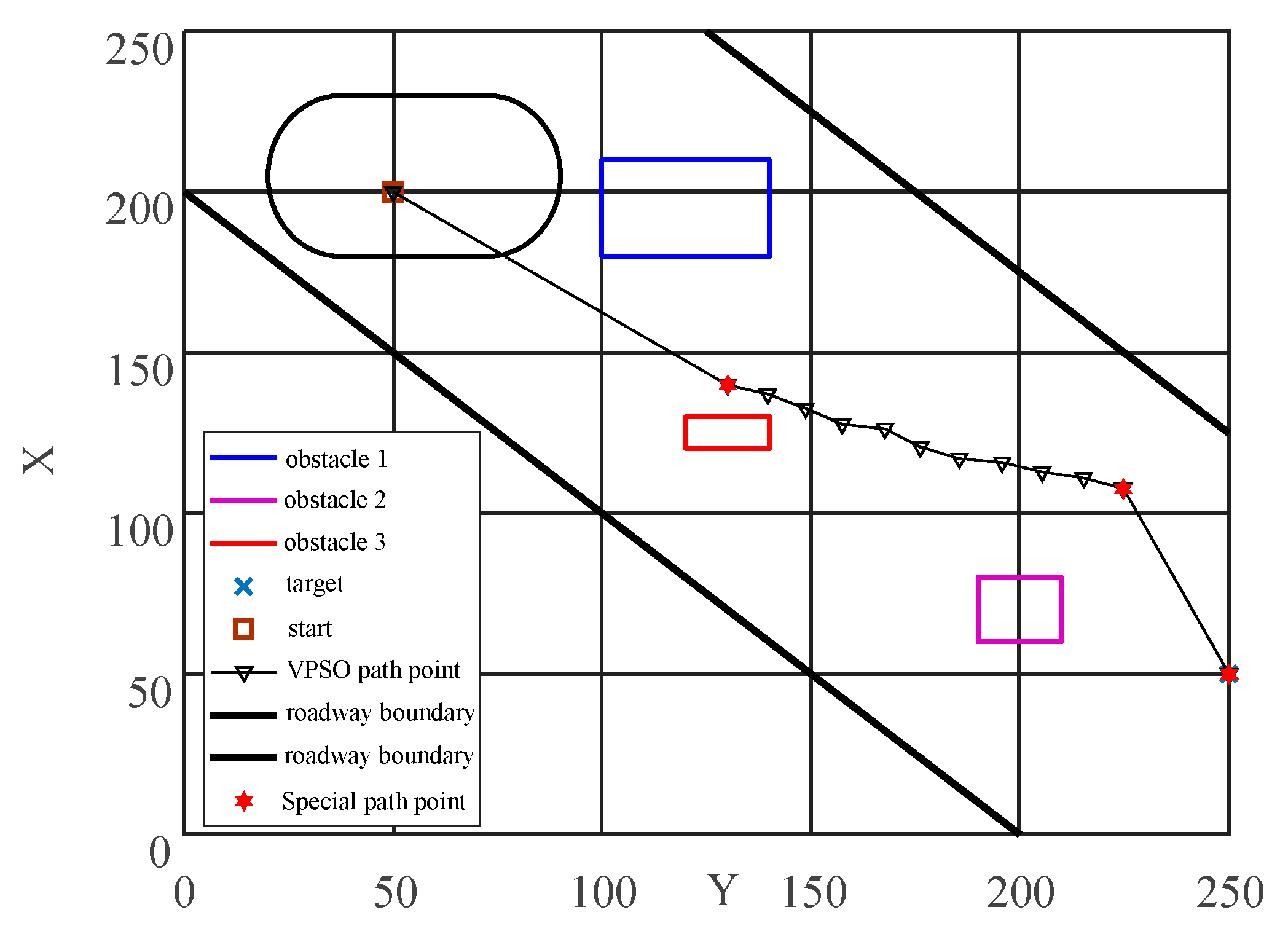
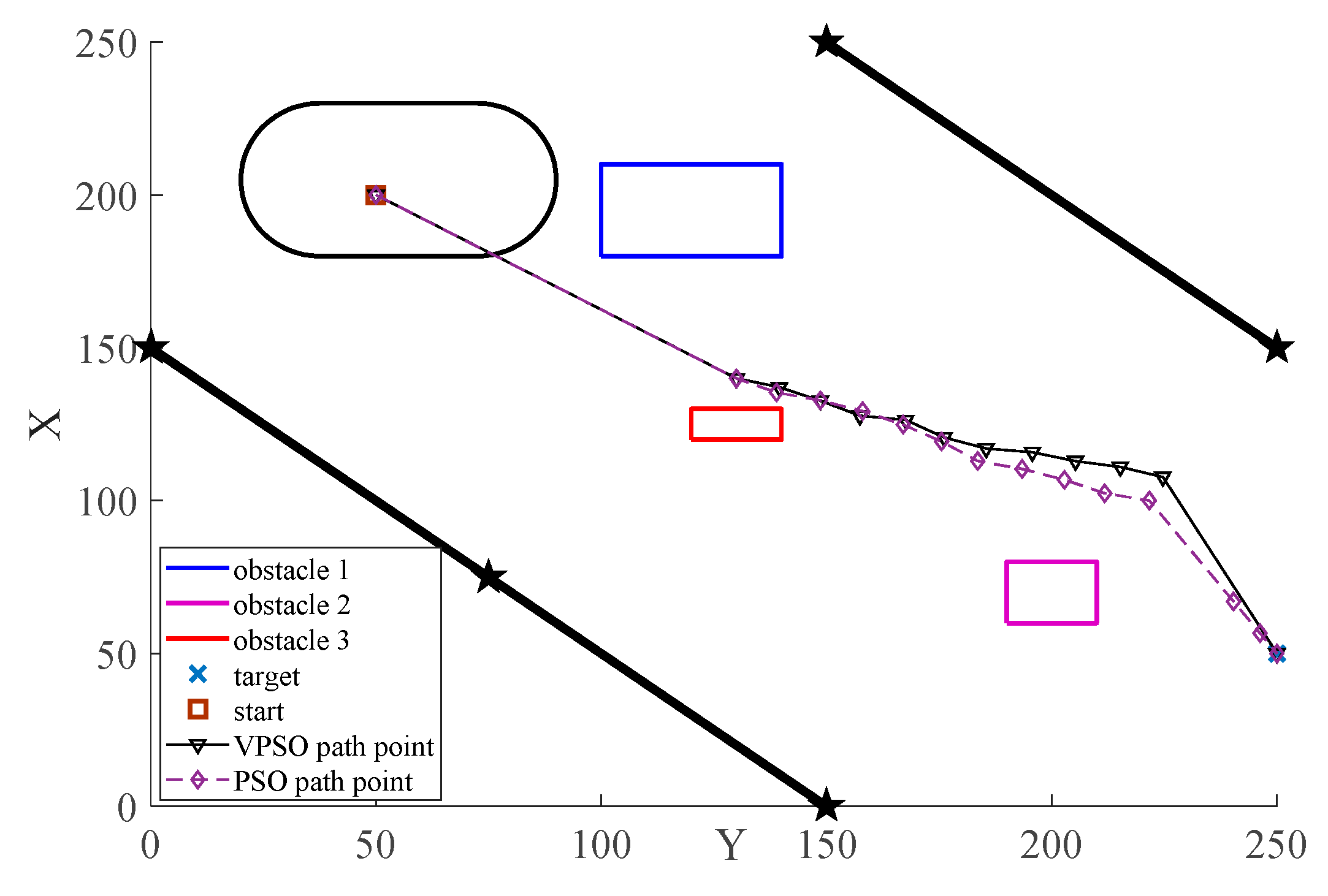
4.1.2. Simulation Analysis of the Roadheader’s Rectification Plan

The roadway environment simulation model of the excavation roadway space is presented in Figure 8. In this model, the obstacle areas are 4.25 m², 0.8 m², and 0.6 m². The influence degrees of the autonomous rectification are 0.415, 0.91, and 0.265. The humidity of the overall roadway soil is 10%. The soil of the simulated floor is a combination of sandy loam soil, powdery coal-type soil, and gravel coal-type soil. The roadheader’s rectification plan simulation of the standard and mutated particle swarm optimization algorithm in this model is presented in Figure 12 and

Table 4. The roadheader’s rectification path plan parameter.

Path Plan Performance Parameters	VPSO	PSO
Sum of centroid displacements (mm)	2570.89	2388.73
Total angle (rad)	1.7091	1.5938
Safety index(mm)	280.293	245.29
Total cost	0.3096	0.3415

.

According to the simulation results, for the total rotation angle and cost, the VPSO algorithm exhibited better performance than the PSO algorithm, and the summation of the centroid displacements was almost the same; however, the VPSO algorithm revealed a significant improvement in safety.

4.1.3. Simulation of the Roadheader Rectifying Point Tracking

Initially, the rectification points should be found in the rectification area and then tracked based on the positions of these special points. Three special points can be selected among the roadheader’s rectification path plan points, then the roadheader can track these marked points. According to the marked points, the total length, total angle, total cost, and safety index of this path can be obtained. A comparison between the special rectification points tracking and the original points tracking is presented in Figure 13 and

Table 5. Simulation parameters of the point-searching algorithm.

Parameter	Original Points Track	Marked Points Track
Total distance(mm)	2570.89	2097.14
Total angular rotation (rad)	1.7091	1.5777
Safety index (mm)	280.293	280.293
cost index	0.3096	0.3368

.

According to Table 5, this special rectification points tracking algorithm can greatly reduce the number of roadheader movements and thus the cumulative error. At the same time, the rectification safety and control accuracy of the roadheader can be ensured.

5. Conclusions

In this paper, a path rectification planning control algorithm based on variable particle swarm optimization is proposed based on the actual working conditions of mine tunneling, and the effectiveness and practicability of this path planning method is verified by simulation. This method provides a theoretical basis for the realization of intelligent path rectification of a roadheader, provides technical support for the realization of unmanned tunneling work, and improves the safety and efficiency of coal mine tunneling production.

(1) Based on the actual working conditions of roadways in coal mines, this paper fully considered the problems encountered in normal roadheader operation, including compaction resistance, bulldozing resistance, steering resistance, tunnel dip angle, ditching, and obstacle-crossing capacity. The driving performance of a roadheader was analyzed, and a resistance model of a roadheader crawler traveling on a roadway floor was established. The kinematic and dynamic models of the roadheader were established by comprehensively considering the roadway conditions and resistances. The validity of the model was verified experimentally. Reliable kinematic and dynamic models were provided for the path rectification planning of roadheaders.

(2) Based on the actual working conditions of tunneling roadways, a grid model of the roadway environment under complex working conditions was established. The parameters rectification impact degree (RID), rectification cost (RC), rectification safety index (RSI), and energy consumption index (ECI) were proposed to simplify the constraints of pre-existing grid models and enhance path rectification planning. A roadheader’s path rectification planning and tracking algorithm based on a variation of the particle swarm optimization algorithm was proposed using the roadway grid model. This algorithm was based on actual working conditions and improved upon the particle swarm optimization algorithm, which can correct the rectification planning of roadheaders accurately, and improve tracking efficiency and accuracy.

(3) To analyze the proposed kinematic and dynamic models and the tracking algorithm for rectification planning, simulation experiments of the EBZ-55 roadheader were carried out. The simulation results verified the effectiveness of, and the improvement afforded by the proposed algorithm.

References

1. Janarthan, B.; Padmanabhan, C.; Sujatha, C. Longitudinal dynamics of a tracked vehicle: Simulation and experiment. J. Terramech. 2012, 49, 63–72. [Google Scholar] [CrossRef]
2. Zang, F.Y.; Liu, D.; Lv, F.Y. Study on anti-skid control of roadheaders on roadways floors with varied dipangles. Coal Sci. Technol. 2019, 47, 30–36. [Google Scholar]
3. Lu, Y.; Xiao, S.; Ge, Z.; Zhou, Z.; Deng, K. Rock-breaking properties of multi-nozzle bits for tree-type drilling in underground coal mines. Energies 2016, 9, 249. [Google Scholar] [CrossRef] [Green Version]
4. Chao, D.; Kai, C.; Xueliang, G.; Yuan, X.; Zhaoyin, D. Tracked vehicle skid steer performance analysis under the influence of centrifugal force. J. Vib. Meas. Diagn. 2017, 37, 76–83. [Google Scholar]
5. Qinglu, S.; Fengchun, S. Study on steering stability of tracked vehicles and ramp. Trans. Chin. Soc. Agric. Mach. 2007, 38, 22–26. [Google Scholar]
6. Zeng, Y.H.; Zhou, Y.C.; Liu, D.C.; Zuo, Q.S. A smart calibration model on track’s pressure–sinkage characteristic of a tracked vehicle moving on soft seabed sediments. J. Cent. South Univ. 2013, 20, 9112–9917. [Google Scholar] [CrossRef]
7. Thueer, T. Mobility evaluation of wheeled all-terrain robots. J. Robot. Auton. Syst. 2010, 58, 508–519. [Google Scholar] [CrossRef]
8. Keiji, N.; Dadisuke, E.; Kazuya, Y. Improvement of the odometry accuracy of a crawler vehicle with consideration of slippage. In Proceedings of the 2007 IEEE International Conference on Robotics and Automation, Roma, Italy, 10–14 April 2007; pp. 2752–2757. [Google Scholar]
9. Feng, C. Study on Deep Seabed Mining Robot Vehicle Motion Modeling and Control. Ph.D. Thesis, Central South University, Changsha, China, 2005. [Google Scholar]
10. Yihui, Z. Research on the Mechanical of Running Behavior Tracked Vehicle Collector in the Soft Sediment and Simulation Test. Ph.D. Thesis, Central South University, Changsha, China, 2013. [Google Scholar]
11. Haohan, S. Reseach on Path Planing of Tracked Unmanned Platform in Dynamic Environment. Ph.D. Thesis, Harbin Institute of Technology, Harbin, China, 2020. [Google Scholar]
12. Chen, S.; Niu, J.; Wen, S.; Chen, Y. Measurement Method of Navigation System of Self-propelled Underground Tunneling Robots. J. Beijing Univ. Technol. 2014, 40, 1091–1098. [Google Scholar]
13. Zhizhong, L. Research on Mechanism Design and Analysis for Robotization of Coal Road Driving Equipment for Soft and Outburst Coal Seam. Ph.D. Thesis, Northeastern University, Boston, MA, USA, 2015. [Google Scholar]
14. Hong, S.; Choi, J.S.; Kim, H.W.; Won, M.C.; Shin, S.C.; Rhee, J.S.; Park, H.U. A path tracking control algorithm for underwater mining vehicles. J. Mech. Sci. Technol. 2009, 23, 2030–2037. [Google Scholar] [CrossRef]
15. Yuanyuan, Q.; Linke, S.; Xiaodong, J. Study on path planning and tracking of the underground mining roadheader. J. Min. Sci. Technol. 2020, 5, 194–202. [Google Scholar] [CrossRef]
16. Wu, J.; Shen, Y.; Ji, X.; Wang, P.; Jiang, H.; Zheng, W.; Li, Y. Trajectory and deviation perception method of boom-type roadheader. J. China Coal Soc. 2021, 46, 2046–2056. [Google Scholar]
17. Yang, J.; Tang, Z.; Wang, X.; Wang, Z.; Yin, B.; Wu, M. Research on environment modeling and excavation obstacle detection method of mine roadway. Coal Sci. Technol. 2020, 48, 12–18. [Google Scholar]
18. Minjun, Z.; Rong, C.; Yu, Z.; Ming, Z.; Fuyu, Z.; Miao, W. Study on roadheader rectification running performance and control in the incline coalmine roadway. J. China Coal Soc. 2021, 46, 310–320. [Google Scholar] [CrossRef]
19. Cheluszka, P. Optimization of the Cutting Process Parameters to Ensure High Efficiency of Drilling Tunnels and Use the Technical Potential of the Boom-Type Roadheader. Energies 2020, 13, 6597. [Google Scholar] [CrossRef]
20. Joostberens, J.; Pawlikowski, A.; Prostański, D.; Nieśpiałowski, K. Method for Assessment of Operation of Analog Filters Installed in the Measuring Lines for Electrical Quantities of a Mining Machine’s Converter Power Supply System. Energies 2021, 14, 2384. [Google Scholar] [CrossRef]
21. Wong, J.Y.; Chiang, C.F. A general theory for skid steering of tracked vehicles on firm ground. J. Automob. Eng. 2001, 21, 52–57. [Google Scholar] [CrossRef]
22. Kejian, Z. Terrain Vehicle Mechanics; Duo, Y., Ma, C., Eds.; National Defence Industry Press: Beijing, China, 2002; ISBN 711802564X. [Google Scholar]
23. Acaroglu, O.; Erdogan, C. Stability analysis of roadheaders with mini-disc. Tunn. Undergr. Space Technol. 2017, 68, 187–195. [Google Scholar] [CrossRef]
24. Suraj, D.; Raina, A.K.; Murthy, V.M.S.R.; Trivedi, R.; Vajre, R. Roadheader-A comprehensive review. Tunn. Undergr. Space Technol. 2020, 95, 103148.1–103148.12. [Google Scholar]
25. Guofa, W.; Desheng, Z. Innovation practice and development prospect of intelligent fully mechanized technology for coal mining. J. China Univ. Min. Technol. 2018, 47, 459–467. [Google Scholar]
26. Huang, Z.; Zhang, Z.; Li, Y.; Song, G.; He, Y. Nonlinear dynamic analysis of cutting head-rotor-bearing system of the roadheader. J. Mech. Sci. Technol. 2019, 33, 1033–1043. [Google Scholar] [CrossRef]
27. Asadi, A.; Abbasi, A.; Bagheri, A. Prediction of Roadheader Bit Consumption Rate in Coal Mines Using Artifificial Neural Networks. In 3rd Nordic Rock Mechanics Symposium-NRMS International Society for Rock Mechanics and Rock Engineering; OnePetro: Richardson, TX, USA, 2017; p. 12. [Google Scholar]
28. Minjun, Z.; Miao, W. Analysis of Vibration of Roadheader Rotary Table Based on Finite Element Method and Data from Underground Coalmine. Shock Vib. 2018, 3, 1–9. [Google Scholar]
29. Park, B.; Choi, J.; Wan, K.C. Sampling-based retraction method for improving the quality of mobile robot path plan. Int. J. Control Autom. Syst. 2012, 10, 982–991. [Google Scholar] [CrossRef]
30. Karlsen, H.H.; Vinter, B. Minimum intrusion Grid-The Simple Model. In Proceedings of the Workshop on Enabling Technologies Infrastructure for Collaborative Enterprises Wet Ice, Linkoping, Sweden, 13–15 June 2005; pp. 305–310. [Google Scholar]
31. Wen, X.M.; Zhao, W.; Meng, F.X. Research of Grid Scheduling Algorithm Based on P2P_Grid Model. In Proceedings of the 2009 International Conference on Electronic Commerce and Business Intelligence, Beijing, China, 6–7 June 2009. [Google Scholar]
32. Heitkoetter, W.; Medjroubi, W.; Vogt, T.; Agert, C. Comparison of Open Source Power Grid Models—Combining a Mathematical, Visual and Electrical Analysis in an Open Source Tool. Energies 2019, 12, 4728. [Google Scholar] [CrossRef] [Green Version]
33. Jiang, J.J.; Wei, W.X.; Shao, W.L.; Liang, Y.F.; Qu, Y.Y. Research on Large-Scale Bi-Level Particle Swarm Optimization Algorithm. IEEE Access 2021, 9, 56364–56375. [Google Scholar] [CrossRef]
34. Li, R.; Zhang, M.; Wang, P.; Shen, Y.; Wu, M. Research on autonomous navigation method for crawler support vehicle based on regional grid. J. Min. Sci. Technol. 2020, 5, 423–434. [Google Scholar]
35. Viet, D.T.; Phuong, V.V.; Duong, M.Q.; Tran, Q.T. Models for Short-Term Wind Power Forecasting Based on Improved Artificial Neural Network Using Particle Swarm Optimization and Genetic Algorithms. Energies 2020, 13, 2873. [Google Scholar] [CrossRef]
36. Lei, H. A review of particle swarm optimization algorithms. Mech. Eng. Autom. 2010, 5, 197–199. [Google Scholar]
37. Jian-Hu, F.; Ting-Yu, Z.; Shuo, F.; Bao-Juan, Z. Improved Particle Swarm Optimization Algorithm for Robot Path Planning. Mach. Des. Manuf. 2021, 9, 291–298. [Google Scholar]
38. Guanghui, G. Ultra-wideband Positioning Method Based on Particle Swarm Optimization for Tunneling Support Bracket. Ph.D. Thesis, China University of Mining and Technology, Xuzhou, China, 2019. [Google Scholar]
Figure 1. Friction between the roadheader and roadway.
Energies 14 07201 g001
Figure 2. Roadheader steering diagram on an inclined roadway.
Energies 14 07201 g002
Figure 3. Dynamics diagram of roadheader’s rectification.
Energies 14 07201 g003
Figure 4. Analysis of roadheader’s driving performance, (a) Analysis of ditching capacity, (b) Analysis of obstacle crossing ability.
Energies 14 07201 g004
Figure 5. Site of the uniform motion experiment.
Energies 14 07201 g005
Figure 6. Experimental site of the turning motion on slope experiment.
Energies 14 07201 g006
Figure 7. Experimental data of uniform motion, (a) Driving Torque of Calculation and Measuring, (b) Deviation Torque.
Energies 14 07201 g007
Figure 8. Experimental data of turning motion on slope, (a) Driving Torque of Calculation and Measuring, (b) Deviation Torque.
Energies 14 07201 g008
Figure 9. Schematic diagram of roadway environment modeling.
Energies 14 07201 g009
Figure 10. The variable particle swarm in the rectification plan.
Energies 14 07201 g010
Figure 11. The minimum fitness curve of the two algorithms, PSO and VPSO, (a) The fitness variation of A function, (b) The fitness variation of G function.
Energies 14 07201 g011
Figure 12. Simulation of the roadheader’s rectification path plan.
Energies 14 07201 g012
Figure 13. Simulation of the rectification points searching and tracking algorithm.
Energies 14 07201 g013