
Multi-Time-Scale Optimal Scheduling in Active Distribution Network with Voltage Stability Constraints

Abstract
:1. Introduction
- A voltage stability index is proposed based on the Jacobian of Distflow branch flow model with no assumption. The index is a linear function of the locally measurable power flow variables. The simulation shows that the index has the same change trend as the common index load margin over the time horizon. A linear voltage stability constraint is proposed by using the index and can be embedded in the optimization problem of the radial distribution networks without increasing the computational burdens.
- The VSCOS model is formulated as a multi-time-scale framework. The day-ahead model coordinates different types of devices to guarantee the voltage stability and minimize the network losses. To cope with the uncertainty of the loads and the renewable energy, the intra-day model reschedules the PV converters and the ESSs on a shorter fine-grained time scale.
2. Voltage Stability Constraints for a Radial Distribution Network
2.1. Radial Distribution Network Model
2.2. Voltage Stability Constraint
- First of all, the main advantage is its good linearity with respect to the decision variables. According to the definition of the index , the proposed voltage stability constraint of an arbitrary bus is a linear constraint and does not introduce any new variables. Therefore, it can be conveniently and directly integrated into the optimal scheduling and planning problems and cause no additional computational burdens.
- Second, because all nodes in are treated as PQ buses, the effect of the dynamic characteristics of the power injection and consumption on voltage stability cannot be considered in this model. Hence, the proposed constraint is essentially a steady-state voltage stability constraint. However, the aim of this paper is to ensure a safe voltage stability margin by coordinating various devices in the ADNs, so the proposed constraint is sufficiently effective. Nevertheless, it is important to point out that this constraint is not recommended when studying the short-term stability of the distribution networks hosting a large number of loads with dynamic voltage response characteristics.
- Furthermore, the voltage stability constraint is applicable to balanced radial distribution networks. Although it is common that distribution networks are designed as loop topology and operated with radial network arrangements, extending the proposed constraint to all possible arrangements (i.e., radial, mesh, and loop) is a potential future improvement. As an increasing number of plug-in loads (especially electric vehicles) and behind-the-meter rooftop PVs are connected to the distribution networks through a single phase, it is promising to study the extension of the voltage stability constraint to unbalanced three-phase networks.
3. Multi-Time-Scale Optimal Scheduling Model
3.1. Controllable Device Model
3.1.1. On-Load Tap Changer
3.1.2. Energy Storage System
3.1.3. Capacitor Bank
3.1.4. PV Converter
3.2. Day-Ahead Optimal Scheduling
3.3. Intra-Day Corrective Adjustment
4. Case Study
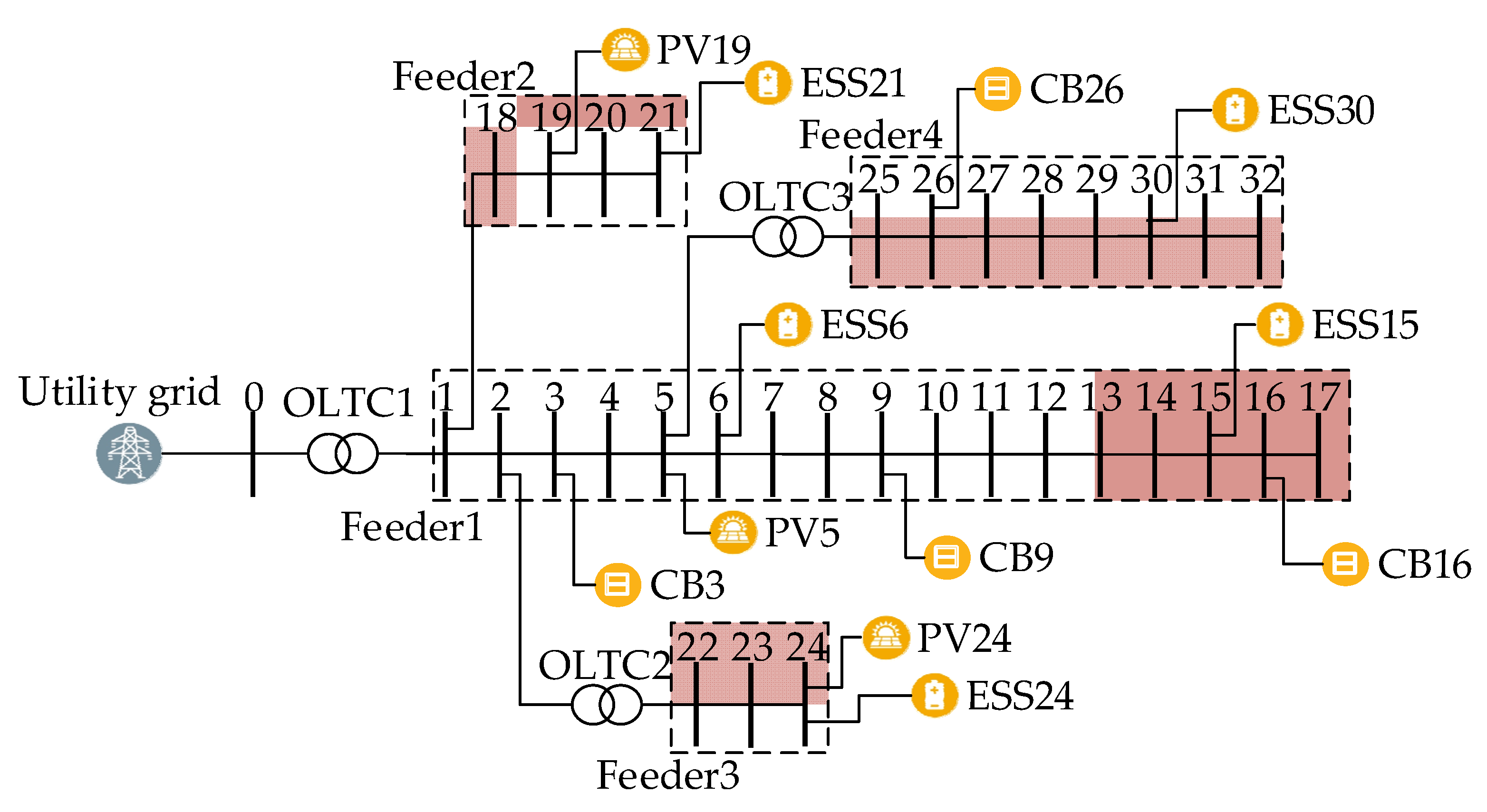
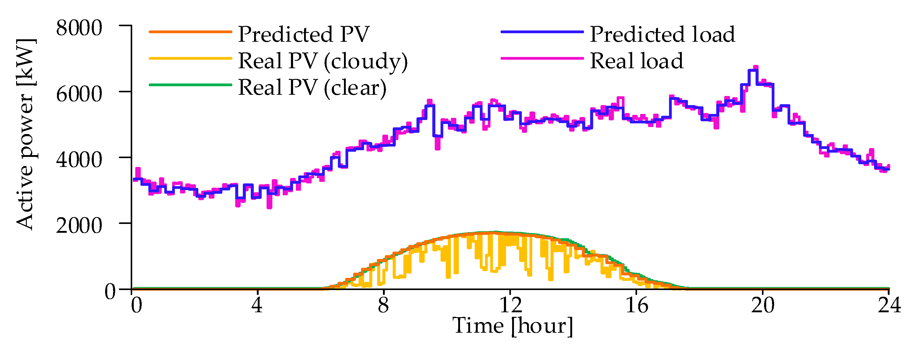
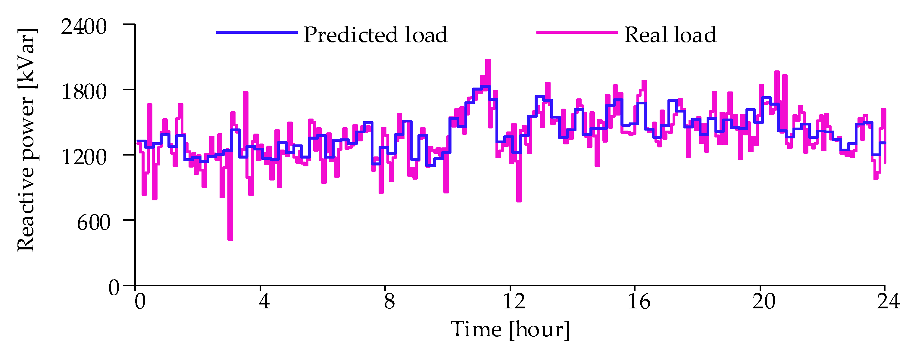
4.1. Test System
4.2. Simulation Results and Analysis
4.2.1. Day-ahead Scheme Obtained by the VSCOS Model
4.2.2. Effect of the Voltage Stability Constraint on Day-Ahead Scheme
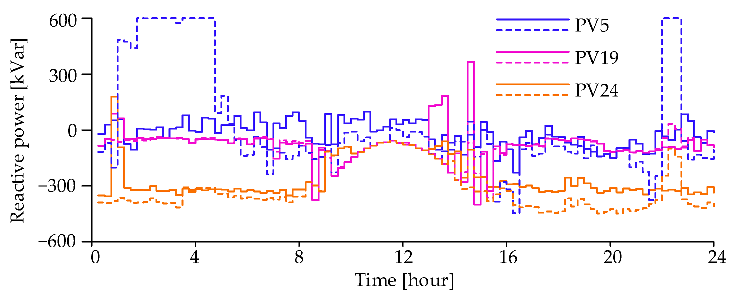
- The distribution network operator is the owner of the PVs or has full authority over the PVs. For the purposes of economic operation, the operator requires the PV converters to output a large amount of reactive power. The case study in this paper is consistent with this situation.
- In a competitive market, the PV entities can be encouraged to output a large amount of reactive power by an effective compensation mechanism or market price signal. For the sake of profit, the active power generation can even be reduced to make way for reactive power. It is noteworthy that the PV converters may no longer adopt the maximum power point tracking control in this scenario.
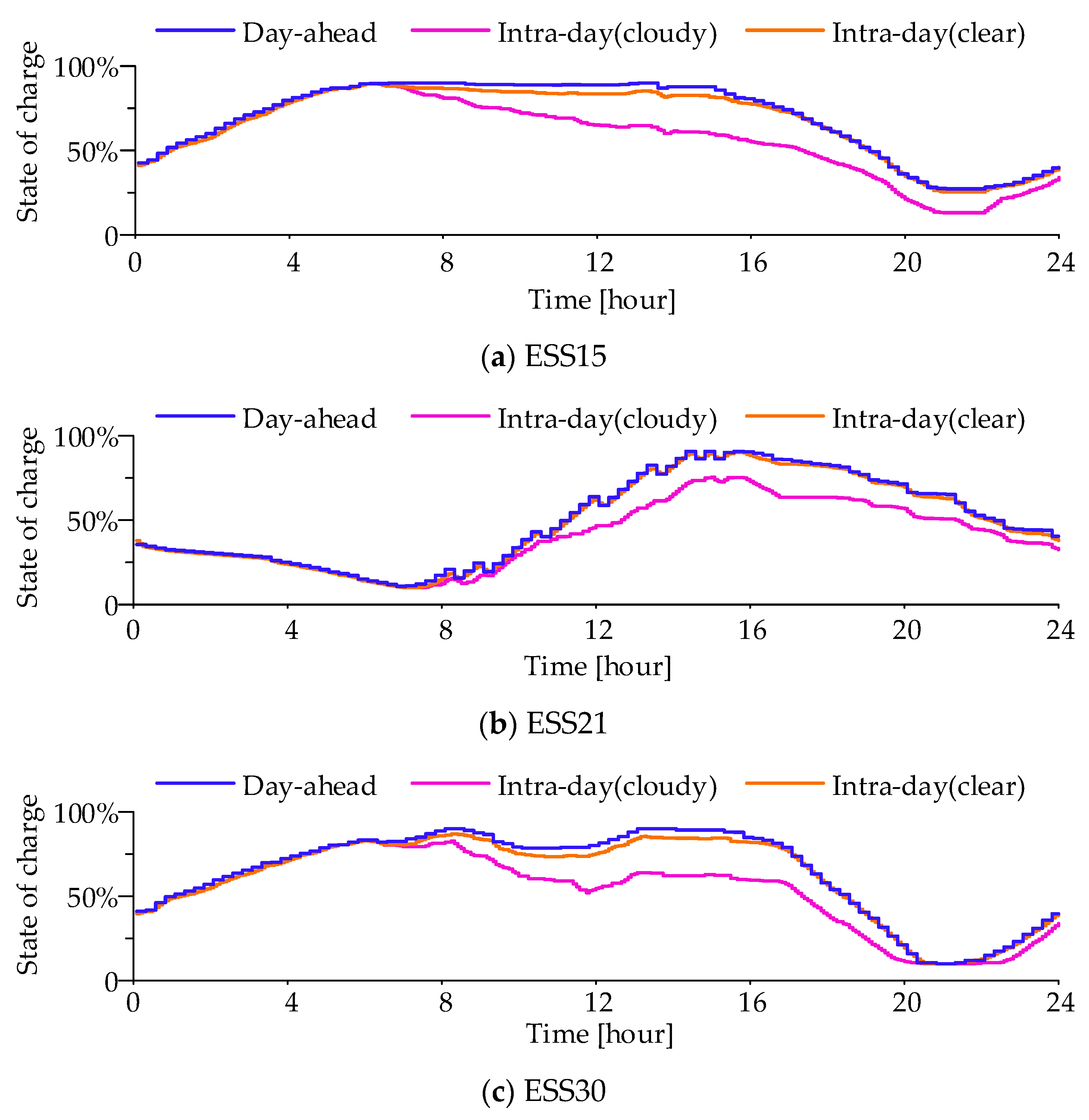
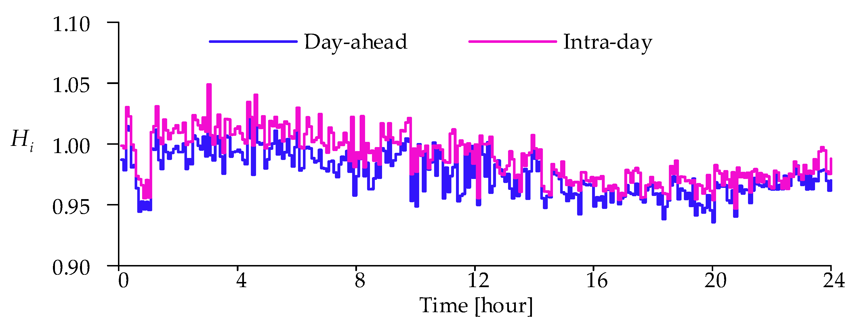
4.2.3. Intra-Day Scheme under Cloudy Sky Conditions
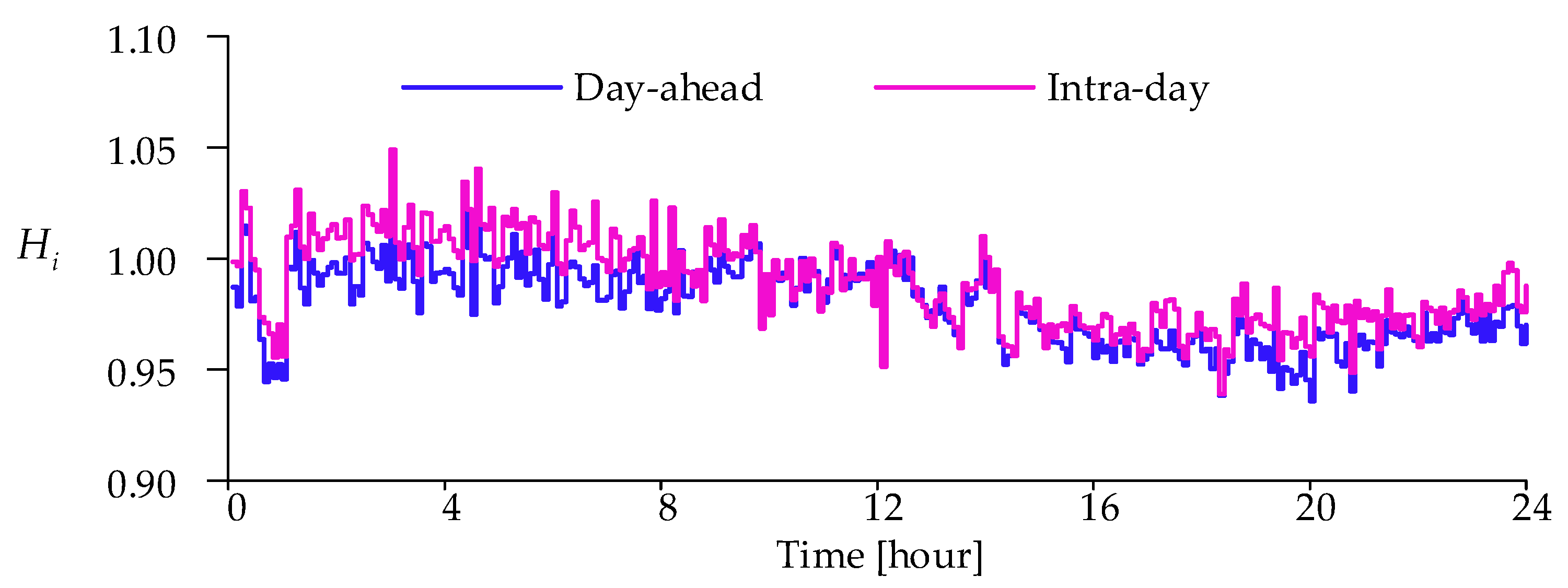
4.2.4. Intra-Day Scheme under Clear Sky Conditions
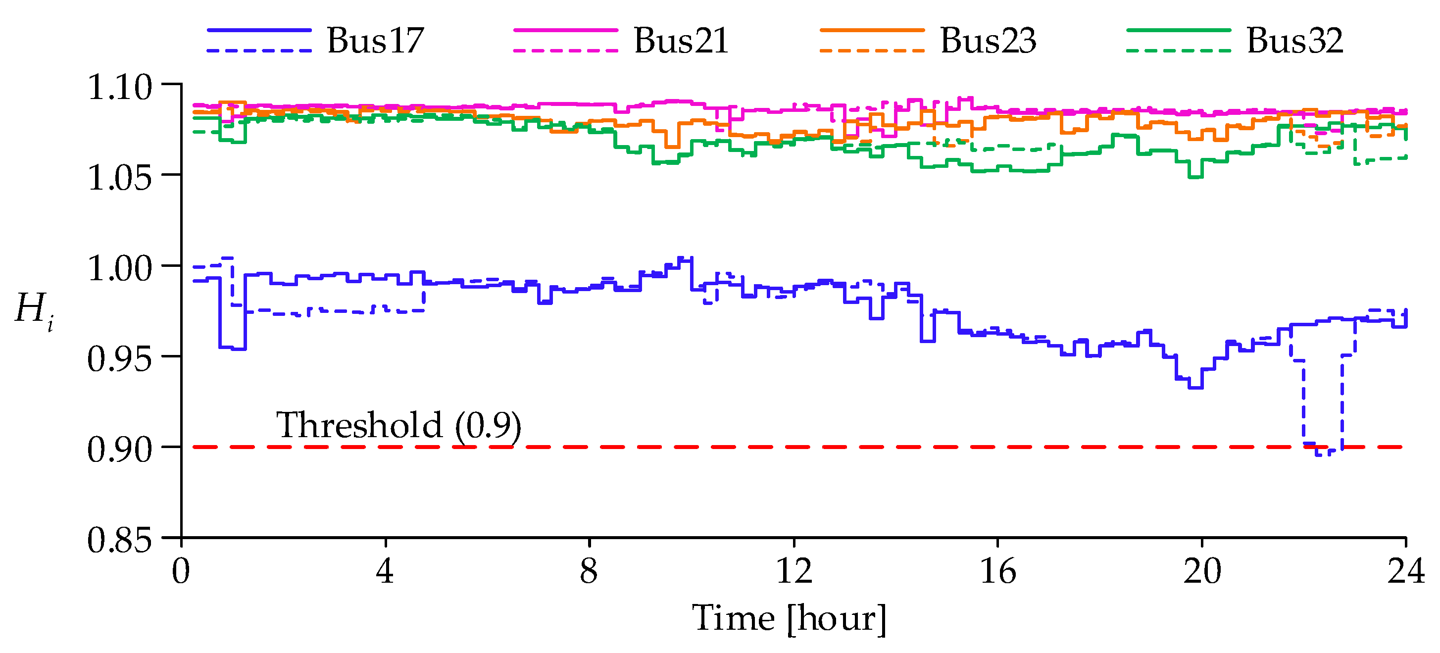
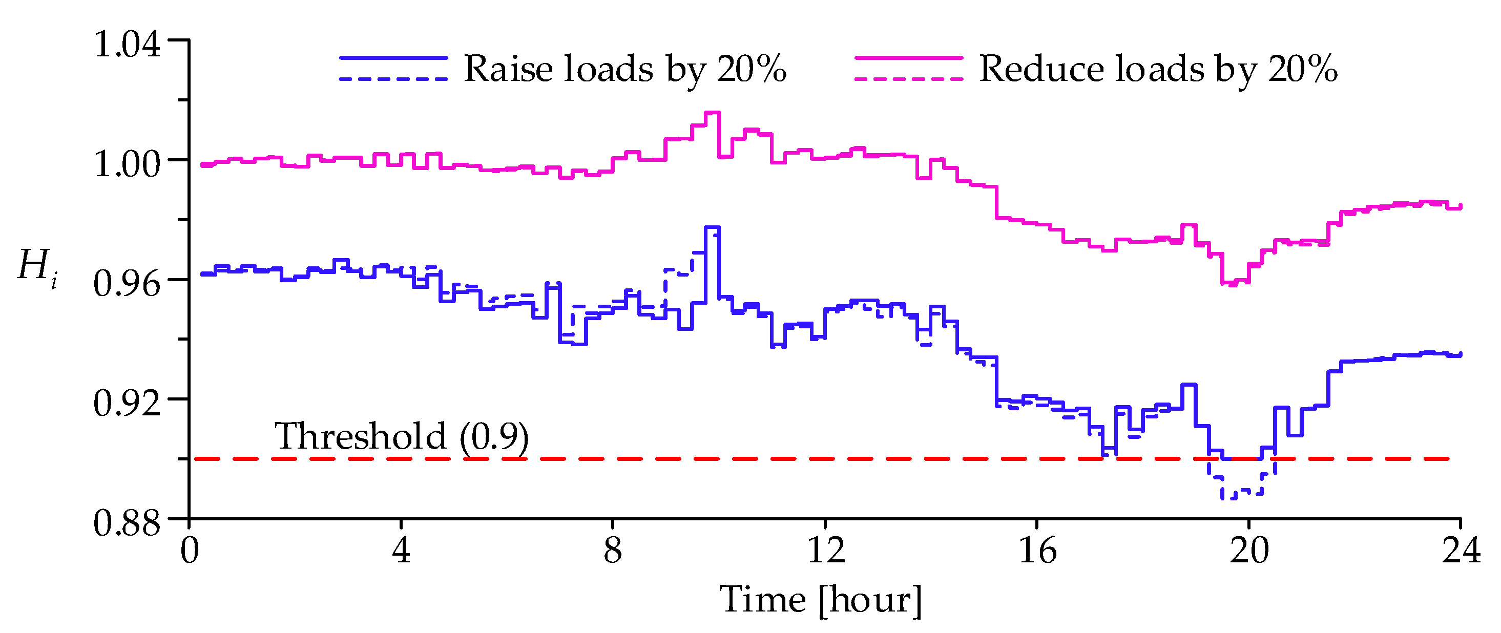
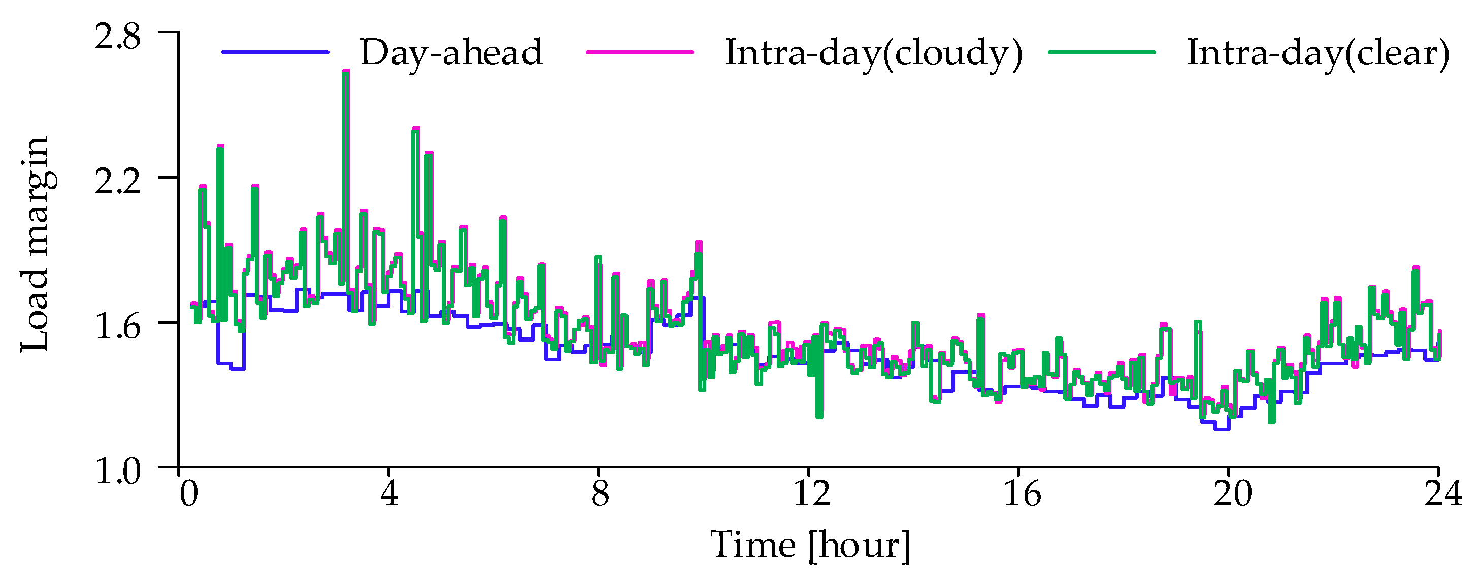
4.2.5. Effectiveness of the Proposed Voltage Stability Index
4.2.6. Computational Time Comparison
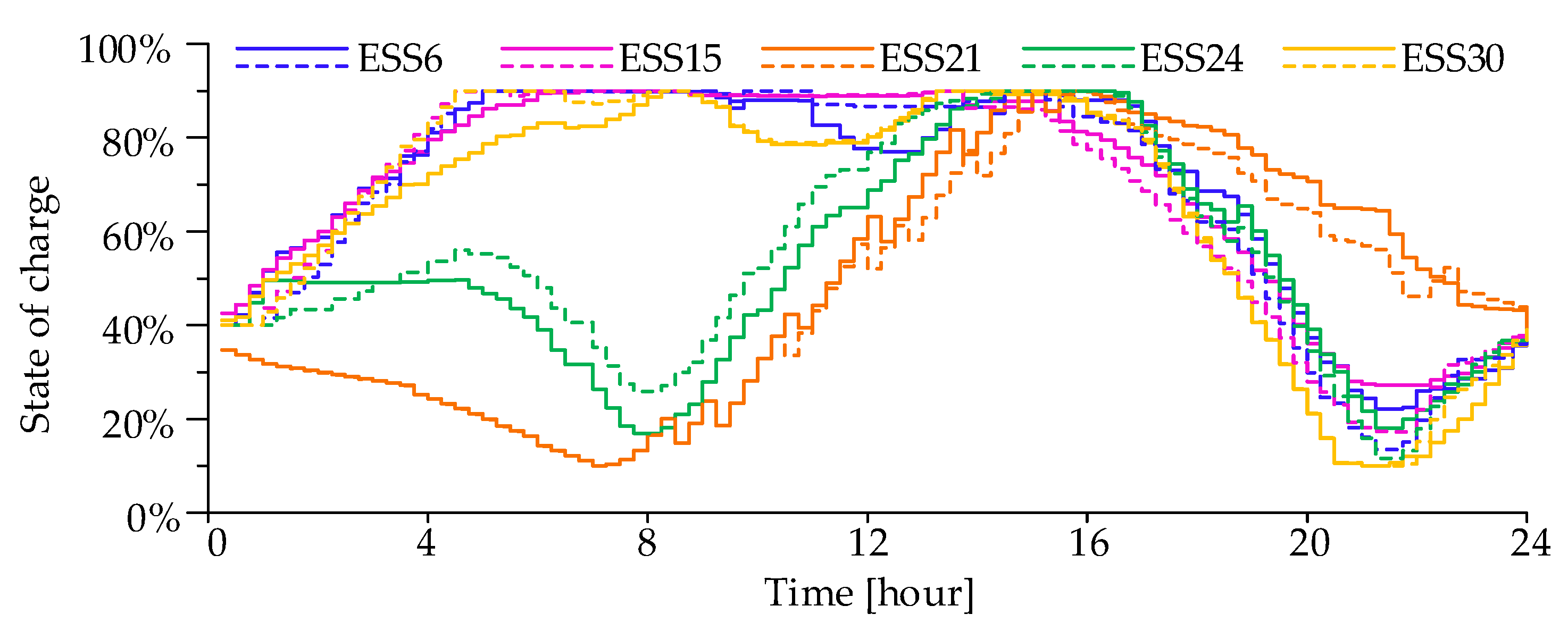
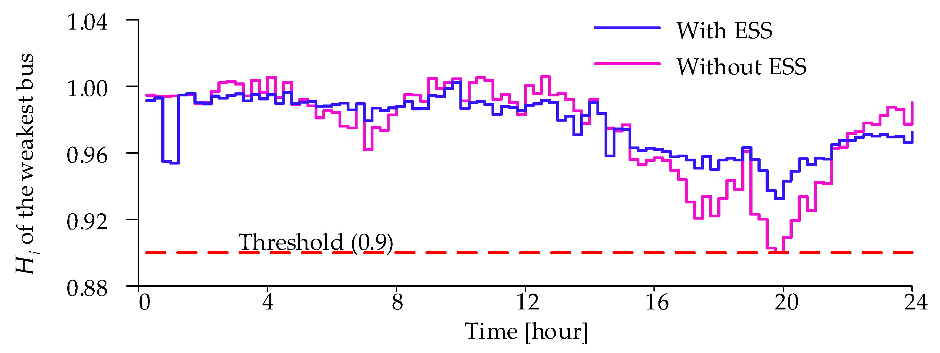
4.2.7. Effect of ESS on Voltage Stability
5. Conclusions
Author Contributions
Funding
Institutional Review Board Statement
Informed Consent Statement
Data Availability Statement
Conflicts of Interest
References
- Sultana, U.; Khairuddin, A.B.; Aman, M.M.; Mokhtar, A.S.; Zareen, N. A review of optimum DG placement based on minimization of power losses and voltage stability enhancement of distribution system. Renew. Sustain. Energy Rev. 2016, 63, 363–378. [Google Scholar] [CrossRef]
- Ghosh, S.; Rahman, S.; Pipattanasomporn, M. Distribution Voltage Regulation Through Active Power Curtailment With PV Inverters and Solar Generation Forecasts. IEEE Trans. Sustain. Energy 2017, 8, 13–22. [Google Scholar] [CrossRef]
- Ajjarapu, V.; Christy, C. The continuation power flow: A tool for steady state voltage stability analysis. IEEE Trans. Power Syst. 1992, 7, 416–423. [Google Scholar] [CrossRef]
- Rabiee, A.; Mohseni-Bonab, S.M.; Parniani, M.; Kamwa, I. Optimal Cost of Voltage Security Control Using Voltage Dependent Load Models in Presence of Demand Response. IEEE Trans. Smart Grid 2019, 10, 2383–2395. [Google Scholar] [CrossRef]
- Liu, S.; Shi, R.; Huang, Y.; Li, X.; Li, Z.; Wang, L.; Mao, D.; Liu, L.; Liao, S.; Zhang, M.; et al. A Data-Driven and Data-Based Framework for Online Voltage Stability Assessment Using Partial Mutual Information and Iterated Random Forest. Energies 2021, 14, 715. [Google Scholar] [CrossRef]
- Bakhtvar, M.; Keane, A. Allocation of Wind Capacity Subject to Long Term Voltage Stability Constraints. IEEE Trans. Power Syst. 2016, 31, 2404–2414. [Google Scholar] [CrossRef] [Green Version]
- Cui, B.; Sun, X.A. A New Voltage Stability-Constrained Optimal Power-Flow Model: Sufficient Condition, SOCP Representation, and Relaxation. IEEE Trans. Power Syst. 2018, 33, 5092–5102. [Google Scholar] [CrossRef] [Green Version]
- Urquidez, O.A.; Xie, L. Singular Value Sensitivity Based Optimal Control of Embedded VSC-HVDC for Steady-State Voltage Stability Enhancement. IEEE Trans. Power Syst. 2016, 31, 216–225. [Google Scholar] [CrossRef]
- Abbasi, S.M.; Karbalaei, F.; Badri, A. The Effect of Suitable Network Modeling in Voltage Stability Assessment. IEEE Trans. Power Syst. 2019, 34, 1650–1652. [Google Scholar] [CrossRef]
- Veerasamy, V.; Wahab, N.I.A.; Ramachandran, R.; Othman, M.L.; Hizam, H.; Devendran, V.S.; Irudayaraj, A.X.R.; Vinayagam, A. Recurrent network based power flow solution for voltage stability assessment and improvement with distributed energy sources. Appl. Energy 2021, 302, 117524. [Google Scholar] [CrossRef]
- Chi, Y.; Xu, Y.; Zhang, R. Many-Objective Robust Optimization for Dynamic VAR Planning to Enhance Voltage Stability of a Wind-Energy Power System. IEEE Trans. Power Deliv. 2021, 36, 30–42. [Google Scholar] [CrossRef]
- Wang, C.; Cui, B.; Wang, Z.; Gu, C. SDP-Based Optimal Power Flow With Steady-State Voltage Stability Constraints. IEEE Trans. Smart Grid 2019, 10, 4637–4647. [Google Scholar] [CrossRef]
- Islam, M.; Nadarajah, M.; Hossain, M.J. Short-Term Voltage Stability Enhancement in Residential Grid With High Penetration of Rooftop PV Units. IEEE Trans. Sustain. Energy 2019, 10, 2211–2222. [Google Scholar] [CrossRef]
- Maharjan, S.; Kumar, D.S.; Khambadkone, A.M. Enhancing the voltage stability of distribution network during PV ramping conditions with variable speed drive loads. Appl. Energy 2020, 264, 114733. [Google Scholar] [CrossRef]
- Saidi, A.S. Investigation of Structural Voltage Stability in Tunisian Distribution Networks Integrating Large-Scale Solar Photovoltaic Power Plant. Int. J. Bifurc. Chaos 2020, 30, 2050259. [Google Scholar] [CrossRef]
- Aristidou, P.; Valverde, G.; Van Cutsem, T. Contribution of Distribution Network Control to Voltage Stability: A Case Study. IEEE Trans. Smart Grid 2017, 8, 106–116. [Google Scholar] [CrossRef] [Green Version]
- Prionistis, G.; Souxes, T.; Vournas, C. Voltage stability support offered by active distribution networks. Electr. Power Syst. Res. 2021, 190, 106728. [Google Scholar] [CrossRef]
- Titare, L.S.; Singh, P.; Arya, L.D.; Choube, S.C. Optimal reactive power rescheduling based on EPSDE algorithm to enhance static voltage stability. Int. J. Electr. Power Energy Syst. 2014, 63, 588–599. [Google Scholar] [CrossRef]
- Ratra, S.; Tiwari, R.; Niazi, K.R.; Bansal, R.C. Optimal Coordinated Control of OLTCs using Taguchi Method to Enhance Voltage Stability of Power Systems. In Proceedings of the 10th International Conference on Applied Energy (ICAE), Hong Kong, China, 22–25 August 2018; pp. 3957–3963. [Google Scholar]
- Tang, Z.; Hill, D.J.; Liu, T. Distributed Coordinated Reactive Power Control for Voltage Regulation in Distribution Networks. IEEE Trans. Smart Grid 2021, 12, 312–323. [Google Scholar] [CrossRef]
- Ma, W.; Wang, W.; Chen, Z.; Wu, X.; Hu, R.; Tang, F.; Zhang, W. Voltage regulation methods for active distribution networks considering the reactive power optimization of substations. Appl. Energy 2021, 284, 116347. [Google Scholar] [CrossRef]
- Jay, D.; Swarup, K.S. A comprehensive survey on reactive power ancillary service markets. Renew. Sustain. Energy Rev. 2021, 144, 119067. [Google Scholar] [CrossRef]
- Jalali, A.; Aldeen, M. Risk-Based Stochastic Allocation of ESS to Ensure Voltage Stability Margin for Distribution Systems. IEEE Trans. Power Syst. 2019, 34, 1264–1277. [Google Scholar] [CrossRef]
- Onlam, A.; Yodphet, D.; Chatthaworn, R.; Surawanitkun, C.; Siritaratiwat, A.; Khunkitti, P. Power Loss Minimization and Voltage Stability Improvement in Electrical Distribution System via Network Reconfiguration and Distributed Generation Placement Using Novel Adaptive Shuffled Frogs Leaping Algorithm. Energies 2019, 12, 553. [Google Scholar] [CrossRef] [Green Version]
- Hu, S.; Xiang, Y.; Zhang, X.; Liu, J.; Wang, R.; Hong, B. Reactive power operability of distributed energy resources for voltage stability of distribution networks. J. Mod. Power Syst. Clean Energy 2019, 7, 851–861. [Google Scholar] [CrossRef] [Green Version]
- Mohseni-Bonab, S.M.; Kamwa, I.; Moeini, A.; Rabiee, A. Voltage Security Constrained Stochastic Programming Model for Day-Ahead BESS Schedule in Co-Optimization of T&D Systems. IEEE Trans. Sustain. Energy 2020, 11, 391–404. [Google Scholar] [CrossRef]
- Katsanevakis, M.; Stewart, R.A.; Lu, J. A novel voltage stability and quality index demonstrated on a low voltage distribution network with multifunctional energy storage systems. Electr. Power Syst. Res. 2019, 171, 264–282. [Google Scholar] [CrossRef] [Green Version]
- Danilo Montoya, O.; Gil-Gonzalez, W.; Arias-Londono, A.; Rajagopalan, A.; Hernandez, J.C. Voltage Stability Analysis in Medium-Voltage Distribution Networks Using a Second-Order Cone Approximation. Energies 2020, 13, 5717. [Google Scholar] [CrossRef]
- Song, Y.; Hill, D.J.; Liu, T. Static Voltage Stability Analysis of Distribution Systems Based on Network-Load Admittance Ratio. IEEE Trans. Power Syst. 2019, 34, 2270–2280. [Google Scholar] [CrossRef]
- Farivar, M.; Low, S.H. Branch Flow Model: Relaxations and Convexification-Part I. IEEE Trans. Power Syst. 2013, 28, 2554–2564. [Google Scholar] [CrossRef]
- Aolaritei, L.; Bolognani, S.; Dorfler, F. Hierarchical and Distributed Monitoring of Voltage Stability in Distribution Networks. IEEE Trans. Power Syst. 2018, 33, 6705–6714. [Google Scholar] [CrossRef] [Green Version]
- Wang, C.; Gao, R.; Wei, W.; Shafie-khah, M.; Bi, T.; Catalao, J.P.S. Risk-Based Distributionally Robust Optimal Gas-Power Flow With Wasserstein Distance. IEEE Trans. Power Syst. 2019, 34, 2190–2204. [Google Scholar] [CrossRef]
- Faraji, J.; Ketabi, A.; Hashemi-Dezaki, H.; Shafie-Khah, M.; Catalao, J.P.S. Optimal Day-Ahead Scheduling and Operation of the Prosumer by Considering Corrective Actions Based on Very Short-Term Load Forecasting. IEEE Access 2020, 8, 83561–83582. [Google Scholar] [CrossRef]
- Rosewater, D.; Baldick, R.; Santoso, S. Risk-Averse Model Predictive Control Design for Battery Energy Storage Systems. IEEE Trans. Smart Grid 2020, 11, 2014–2022. [Google Scholar] [CrossRef]
- Bouza Allende, G.; Still, G. Solving bilevel programs with the KKT-approach. Math. Program. 2013, 138, 309–332. [Google Scholar] [CrossRef] [Green Version]
- Liu, B.; Liu, F.; Mei, S.; Zhang, X. Optimal power flow in active distribution networks with on-load tap changer based on second-order cone programming. Autom. Electr. Power Syst. 2015, 39, 40–47. [Google Scholar] [CrossRef]
- Zare, A.; Chung, C.Y.; Zhan, J.; Faried, S.O. A Distributionally Robust Chance-Constrained MILP Model for Multistage Distribution System Planning With Uncertain Renewables and Loads. IEEE Trans. Power Syst. 2018, 33, 5248–5262. [Google Scholar] [CrossRef]
- GUROBI Optimization. Available online: http://www.gurobi.com (accessed on 3 September 2021).
- Khodr, H.M.; Olsina, F.G.; Jesus, P.M.D.O.-D.; Yusta, J.M. Maximum savings approach for location and sizing of capacitors in distribution systems. Electr. Power Syst. Res. 2008, 78, 1192–1203. [Google Scholar] [CrossRef] [Green Version]
- 141-node-network-results. Available online: https://github.com/llsth/141-node-network-results (accessed on 13 October 2021).


| Model | Solution Time [Second] |
|---|---|
| Day-ahead model with VSC 1 | 9120.73 |
| Day-ahead model without VSC | 8819.94 |
| Intra-day model with VSC | 0.0524 2 |
| Intra-day model without VSC | 0.0463 |
| Case | Solution Time with VSC 1 [Second] | Solution Time without VSC [Second] |
|---|---|---|
| 13.9248 MWh Peak Load | 0.2082 | 0.1917 |
| 15.4720 MWh Peak Load | 0.2088 | 0.1951 |
| 17.0192 MWh Peak Load | 0.2133 | 0.1936 |
Publisher’s Note: MDPI stays neutral with regard to jurisdictional claims in published maps and institutional affiliations. |
© 2021 by the authors. Licensee MDPI, Basel, Switzerland. This article is an open access article distributed under the terms and conditions of the Creative Commons Attribution (CC BY) license (https://creativecommons.org/licenses/by/4.0/).
Share and Cite
Song, T.; Han, X.; Zhang, B. Multi-Time-Scale Optimal Scheduling in Active Distribution Network with Voltage Stability Constraints. Energies 2021, 14, 7107. https://doi.org/10.3390/en14217107
Song T, Han X, Zhang B. Multi-Time-Scale Optimal Scheduling in Active Distribution Network with Voltage Stability Constraints. Energies. 2021; 14(21):7107. https://doi.org/10.3390/en14217107
Chicago/Turabian StyleSong, Tianhao, Xiaoqing Han, and Baifu Zhang. 2021. "Multi-Time-Scale Optimal Scheduling in Active Distribution Network with Voltage Stability Constraints" Energies 14, no. 21: 7107. https://doi.org/10.3390/en14217107
APA StyleSong, T., Han, X., & Zhang, B. (2021). Multi-Time-Scale Optimal Scheduling in Active Distribution Network with Voltage Stability Constraints. Energies, 14(21), 7107. https://doi.org/10.3390/en14217107