Optimising Electrical Power Supply Sustainability Using a Grid-Connected Hybrid Renewable Energy System—An NHS Hospital Case Study

Abstract

This study focuses on improving the sustainability of electrical supply in the healthcare system in the UK, to contribute to current efforts made towards the 2050 net-zero carbon target. As a case study, we propose a grid-connected hybrid renewable energy system (HRES) for a hospital in the south-east of England. Electrical consumption data were gathered from five wards in the hospital for a period of one year. PV-battery-grid system architecture was selected to ensure practical execution through the installation of PV arrays on the roof of the facility. Selection of the optimal system was conducted through a novel methodology combining multi-objective optimisation and data forecasting. The optimisation was conducted using a genetic algorithm with two objectives (1) minimisation of the levelised cost of energy and (2) ${\mathrm{CO}}_2$ emissions. Advanced data forecasting was used to forecast grid emissions and other cost parameters at two year intervals (2023 and 2025). Several optimisation simulations were carried out using the actual and forecasted parameters to improve decision making. The results show that incorporating forecasted parameters into the optimisation allows to identify the subset of optimal solutions that will become sub-optimal in the future and, therefore, should be avoided. Finally, a framework for choosing the most suitable subset of optimal solutions was presented.

1. Introduction

In a recent report [1], the National Health Service of the UK (NHS) outlined plans to reach net-zero emissions by 2040, with an $80\%$ reduction by 2028–2032 compared to 1990 levels. This amounts to around $6.1{\mathrm{MtCO}}_2\mathrm{e}$. The report calls for better utilisation of roof spaces to install on-site renewables, which could save up to 580 ${\mathrm{ktCO}}_2\mathrm{e}$ annually. Furthermore, it was highlighted that earlier adoption will maximise the benefits through the accumulation of reductions overtime. Hospitals have high energy consumption, due to complex building functions, continuous hours of operation, and high density of electrical equipment for diagnosis and treatment [2]. Given that the NHS generates 18% of all emissions deriving from the UK non-domestic buildings [3], adopting ambitious sustainability targets will lead to significant reductions in the carbon footprint of the entire UK.

A hybrid renewable energy system (HRES) can be defined as an energy system with more than one source and at least one renewable generator [4]. HRESs can be grid-connected (GC) or stand-alone (sometimes called micro-grids). The study of HRESs have gained attention due to their potential in providing tailored solutions to local demands at competitive prices. HRESs have benefited from the significant reductions in costs of renewable generators in the past decade [5,6]. GC-HRESs have different architectures or configurations, depending on the components of the system, the existence of storage, and type of electricity (AC or DC). The simplest architecture is grid-PV architecture, where PV modules are connected in parallel to the grid via an inverter and supervised by a controller. The controller monitors grid parameters, such as voltage and frequency, and synchronises the output of he solar array with the grid on a real-time basis [7]. Most of the residential rooftop PV installations fall in this category, where PV output is used in covering the electrical demand and the excess is exported back to the grid. Several studies investigated this type of HRES, interested readers can refer to a recent review by Shen et al. [8].

Another common GC-HRES architecture is the grid-PV-battery combination. In many cases, it is beneficial to store the excess electricity in batteries instead of exporting back to the grid. The excess can then be used in times of high demand offsetting the need to import from the grid during peak times, which can often be more expensive than other times. Optimising the electrical power dispatch strategy is one of the topics that gained attention recently. A study carried out by Shabani et al. [9] concentrated on developing a sophisticated battery model to accurately predict the state of the battery. They used the model to size the HRES system with a battery and found that using the complex battery model helped in accurately predicting the state of charge and electrical power discharge characteristics. Hassan et al. [10] concentrated on the battery power management strategy through a case study, in Australia, of several grid-PV-battery configurations. The study accounted for uncertainties in solar generation and energy consumption patterns using the Monte Carlo method.

High penetration PV systems can cause challenges to the grid operators because of the need for grid upgrade, including upsizing transformers. In a recent study in Switzerland by Sevilla et al. [11], it was found that the PV curtailment can be a more cost-effective solution. However, adding energy storage will mitigate most of the issues of grid upgrading. Furthermore, knowledge of the grid-pricing mechanism plays an important role in the energy management of grid-connected PV-battery systems [12,13,14]. Progress in dynamic pricing is seen as essential for electricity networks to adapt to the high penetration of renewables [14]. Recently, Zhang and Tang [12] studied grid-connected residential PV with battery storage. The grid had a variable tariff; when there was excess energy it could be either stored or exported based on the prices of the exports. They performed single-objective optimisation with the cost as the objective function and their proposed model was able to minimise the cost in different grid-export tariff schemes, such as time-of-use tariff and step tariff.

Healthcare facilities in general, and hospitals in particular, have specific consumption patterns and unique challenges. The demand for energy spans electricity, heat, and cooling. Previous researchers tackled several issues, such as do Espirito and Denilson [15] and Lakjiri et al. [16], who proposed tri-generation plants based on solar energy, to cover electricity, heating, and cooling demands, in hospitals. Furthermore, Jahangir et al. [17] studied the possibility of using HRES to supply electricity to a hospital in Iran. The grid connected-HRES included wind turbines, PV array, diesel generators, and battery banks. It was found that grid-connected PV and WT produced the most favourable results in terms of reduction of LCE and emissions of the system. The recent developments in machine learning had provided data scientist with a wide range of libraries that can be utilised to forecast a time-varying process. Forecasting can be fruitful when dealing with renewable energy sources that has distinct seasonality and trends [18,19]. For example, for a system that has PV cells and batteries, forecasting the carbon intensity can inform the dispatch strategy, whether to store the generated energy or to consume it, depending on the predicated intensity. Several other applications are presented in the literature, such as the study by Abushnaf et al. [13], which used forecasting to estimate the demand of a stand-alone HRES. In this paper, we apply the state-of-the-art forecasting algorithm, i.e., Facebook Prophet [20], to provide the dispatch strategy with the information to optimise its performance. In the context of GC-HRES, forecasting has been used before to predict solar irradiance [21,22], loads [23], and costs [24]. However, emission forecasting is not yet used.

Evolutionary algorithms, such as genetic algorithms and particle swarm, are widely used in optimisation of HRES systems (e.g., the study by Bhandari et al. [25]). In multi-objective optimisation, two or more objectives are defined and the optimisation algorithm attempts to reach the Pareto front solutions. These solutions are said to be non-dominant, which means that any improvement of one objective has to come at the expense of other objectives. This means that, theoretically, all the solutions on the Pareto front are equivalent. Choosing one solution from the set of optimum solutions becomes challenging and therefore meta-heuristic algorithms are usually deployed to aid in decision making.

The aim of this work is to study the feasibility of installing grid-connected HRES in an NHS hospital in south-east England. The feasibility is defined here as a cost-effective solution with maximum ${\mathrm{CO}}_2$ reductions to align with the ambitions of the NHS, to drastically reduce their carbon footprint [1]. The main novelty of the work is by combining multi-objective optimisation with data forecasting to reduce the number of optimal solutions. The optimisations are run iteratively, once using present parameters and twice using projected parameters. Optimum solutions that are projected to become sub-optimal in the future are excluded and the Pareto front is divided into segments. Decision-makers can then have an informed decision on which area of the solution to consider based on the specific objectives. To maximise the applicability of the study, practical constraints (e.g., available roof space, export limits, etc.) are considered. This would help facility managers in other NHS Hospitals to reach an informed decision regarding HRES installations.

The rest of the paper is organised as follows: in Section 2, the methodology is detailed; in Section 3, the forecasting of emissions are presented then optimisation results using existing and forecasting data are presented and discussed. In Section 4, final remarks and future work are presented.

2. Methods

This section outlines the methods adopted to conduct this study including the data used in the simulations, followed by the system architecture, emissions forecasting algorithm, and the mathematical modelling of the GC-HRES.

2.1. Data

This section details the two datasets used in this study. The first represents the electricity data that were collected as part of a previous study [26] conducted in Medway NHS Foundation Trust, in the south-east of England. The second dataset is that of carbon intensity recorded across the UK, which was obtained from an open source online API and can be found at [27]. The particulars of each dataset are detailed in Section 2.1.1 and Section 2.1.2.

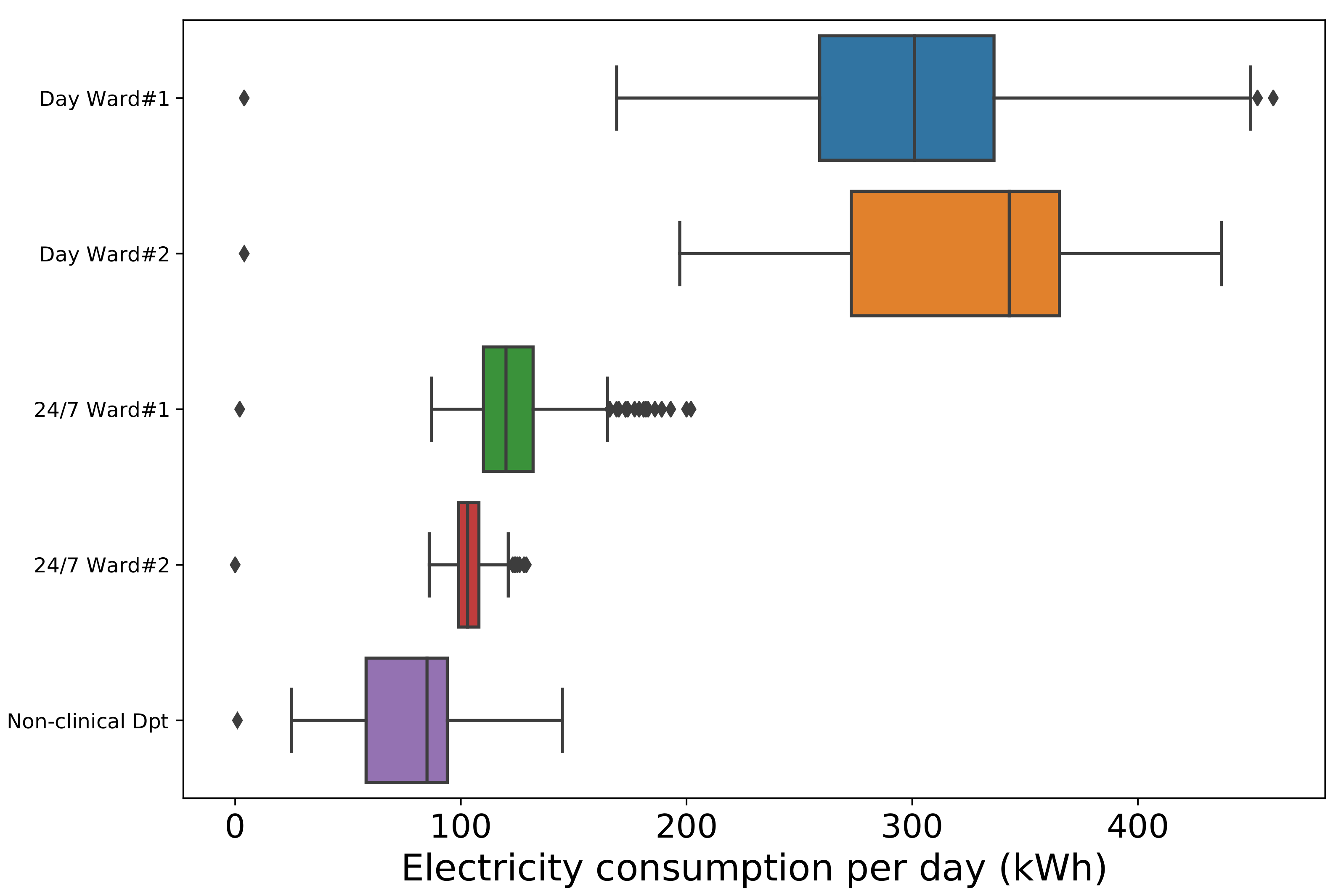
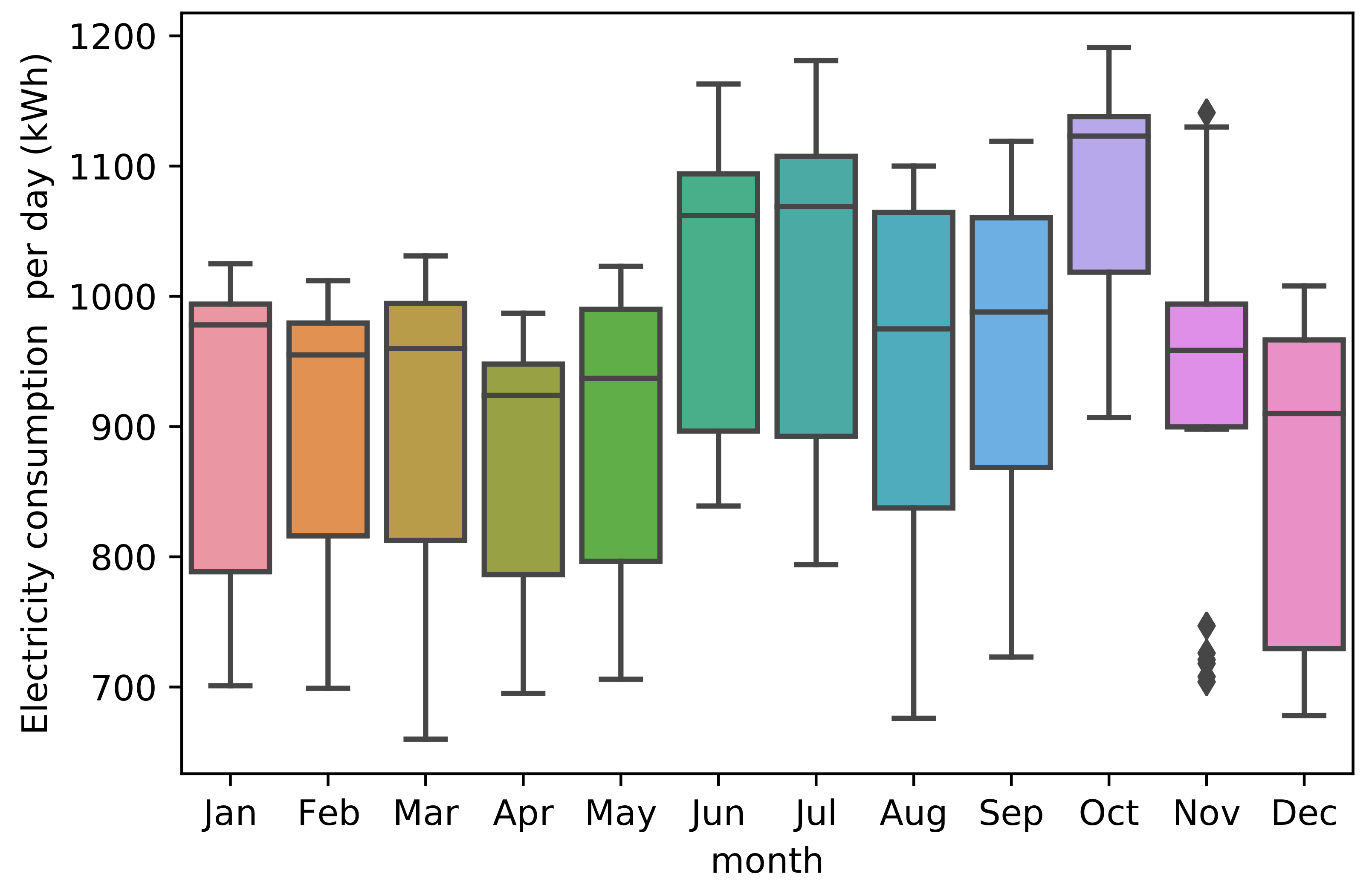
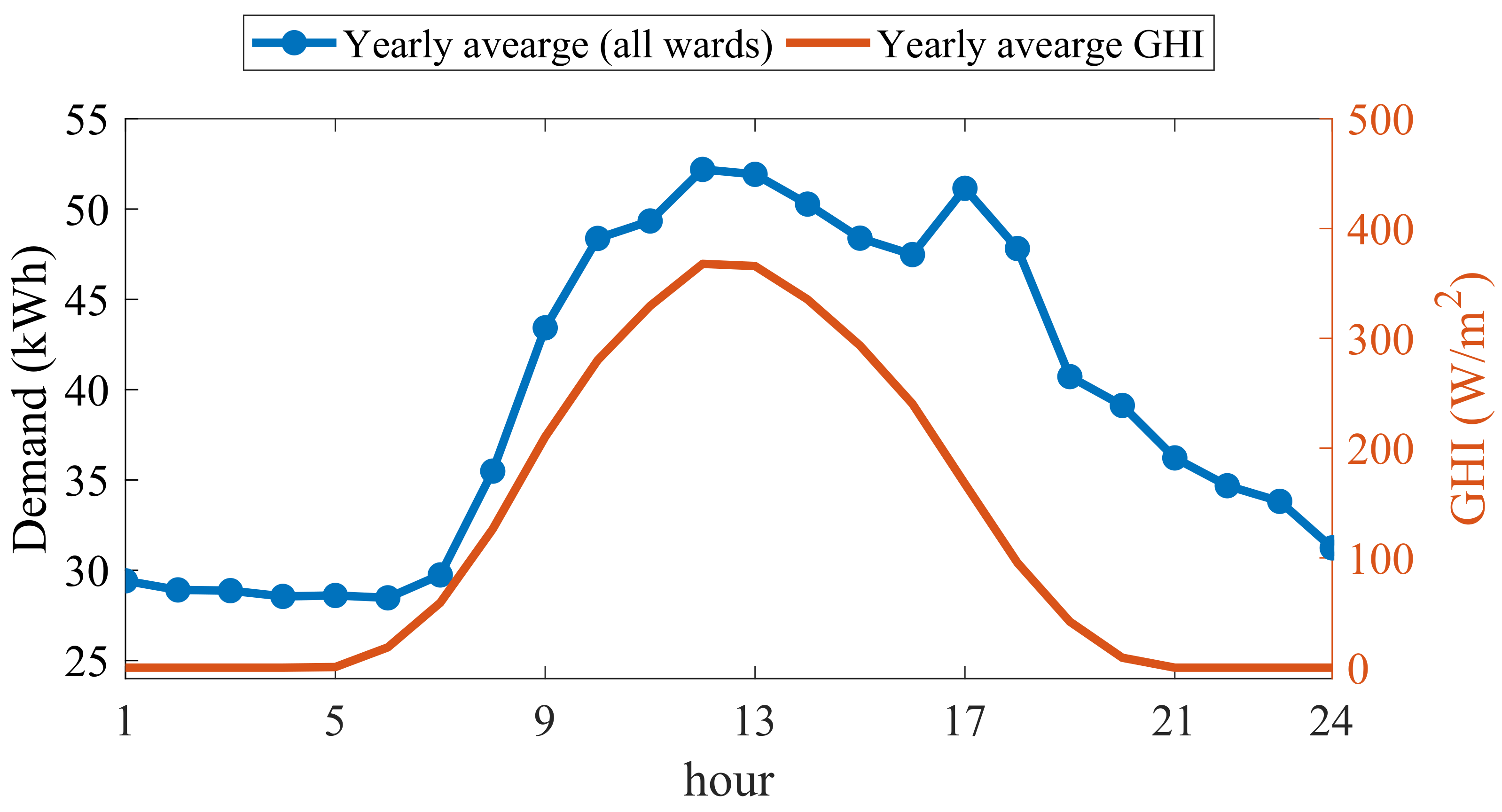
2.1.1. Electricity Consumption Data

The data were collected using a wireless electricity data logger (WEDL), presented in [28], directly from the hospital’s electricity meters. The data spanned a 12-month period, from January 2018 to December 2018, and were recorded at a half-hourly (HH) rate. The electricity meters pulsed 1 kWh pulses, which were collected for half an hour by the WEDL and pushed to the server every hour.

The dataset represents the electricity consumption recorded for five wards/departments from Medway NHS Foundation Trust over the previously mentioned period. It represents a diverse group of wards/departments, including clinical and non-clinical areas, which further strengthens the case for the applicability of the proposed system, primarily to other NHS hospitals and the health sector, but also to other sectors of the society.

The selected five wards/departments can be divided into two categories, the first category, which has four out of the five wards, would incorporate the clinical wards and the second the non-clinical ones, under which comes the fifth department in this study. The clinical category can be subdivided into “Day only” and “$24/7$” wards, two of each were part of this study. Although it is not in the scope of this study, the aim behind the ward selection strategy was to ensure a diversity in the operational nature of each ward/department which would mean various electrical loads and consumption patterns. For instance, Figure 1, shows a box and whisker plot of the daily consumption of the four clinical wards and the non-clinical department in this study. It is clear that the daily median value of the two “$24/7$” wards and the non-clinical department is much less than that of the two “Day” wards, with the minimum value of “Day ward $\#1$” still more than the maximum amongst the two “$24/7$” wards and the non-clinical department.

Although the data were collected for each ward/department, individually, the dataset was combined, in this study, and considered as one, to optimise the HRES based on the collective demand. Accordingly, Figure 2 shows the seasonal demand represented by the selection of wards/departments in this study. As can be seen from the box and whiskers plot, the months of October, July, and June recorded the highest daily median, respectively. However, the demand in other months does not significantly drop as seen in the figure. For instance, the minimum value, recorded in March, is just under 700 kWh and the difference in the medians is between 5% and 10%. This shows the high demand of the selected wards/departments and is a reflection of that of the hospital.

Monthly rates of electricity for the duration of the study were collected and are shown in Figure 3. The variable rate is common for businesses in the UK and depends on consumption. Usually, lower rates are offered to larger consumers. The rates varied between GBP 0.11/kWh to GBP 0.14/kWh, with an exception in the month of March. The rate of GBP 0.025/kWh was considered an outlier and replaced with the mean value of the rest of the readings.

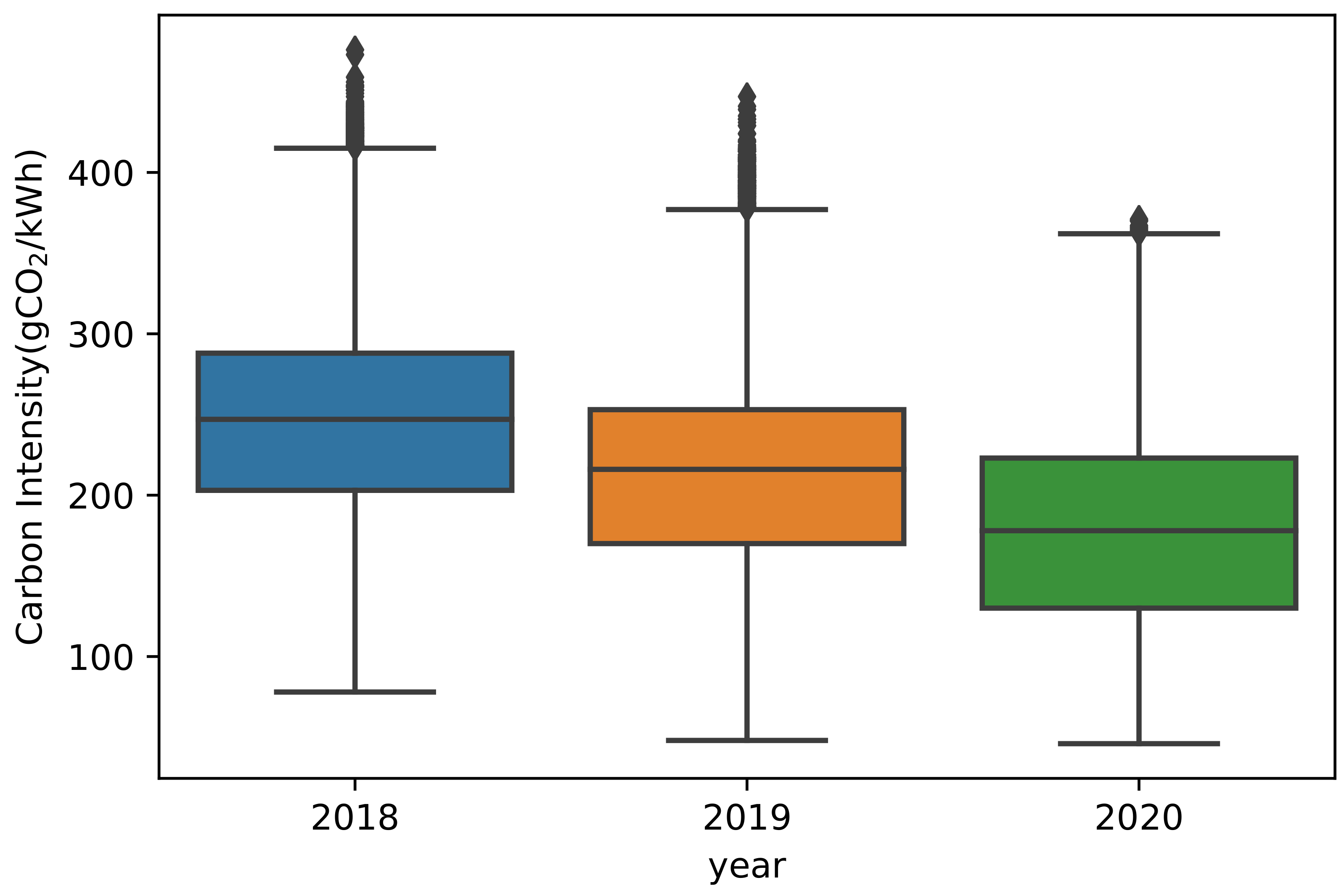
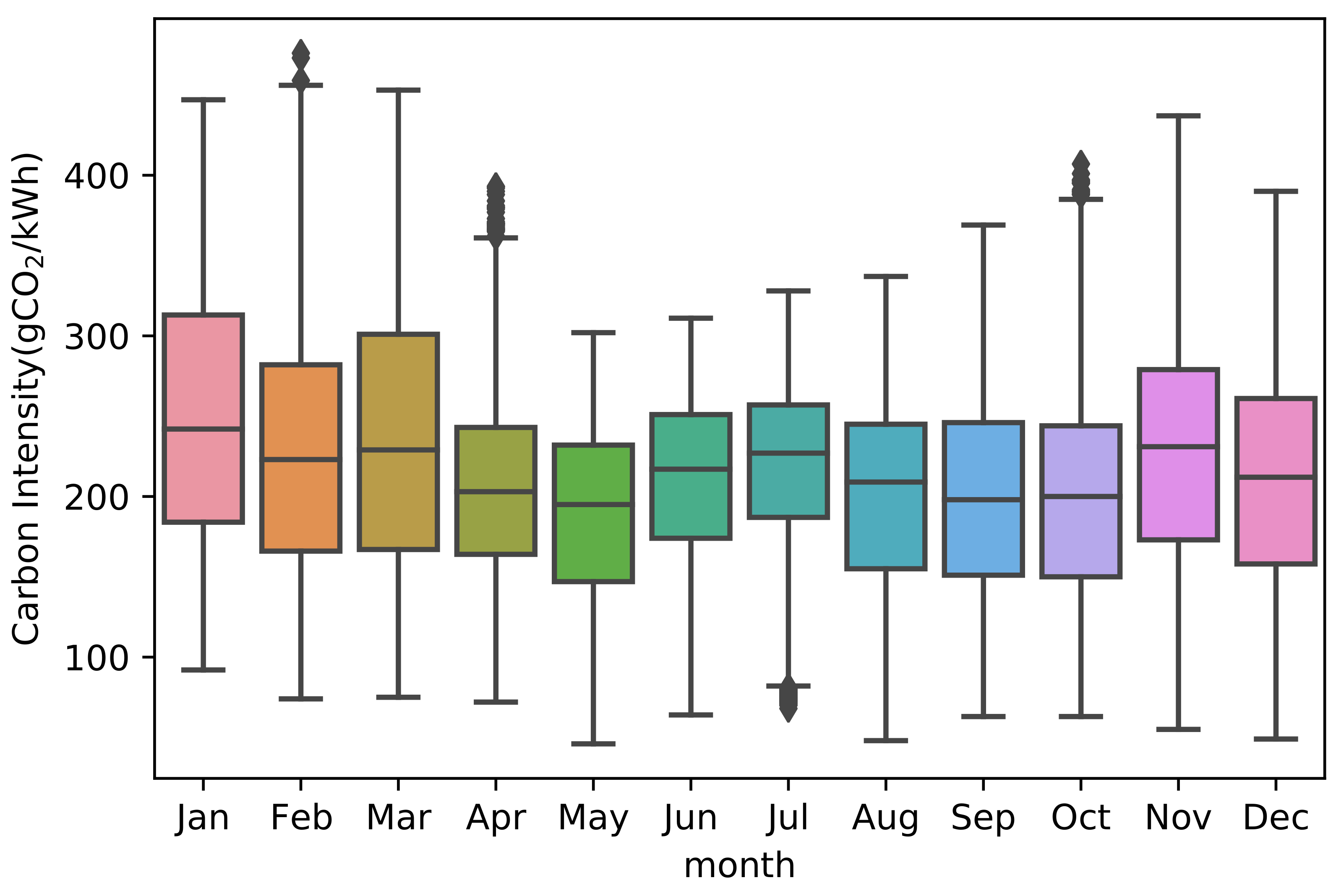
2.1.2. Carbon Intensity

The carbon intensity of electricity is an indicator that shows the amount of CO${}_2$ emissions related to electricity generation only. In Great Britain (GB), the National Grid Electricity System Operator (ESO), in partnership with Environmental Defense Fund Europe and the World Wide Fund for Nature (WWF), have developed a series of regional carbon intensity forecasts for the GB electricity system, with weather data provided by the Met Office [27].

The carbon intensity dataset incorporates CO${}_2$ emissions from all large metered power stations, inter-connector imports, transmission, and distribution losses, and accounts for national electricity demand, and both regional embedded wind and solar generation. The dataset does not consider the CO${}_2$ emissions of un-metered and embedded generators. The GB carbon intensity $C_t$ time t is found by weighting the carbon intensity $c_g$ for fuel type g by the generation $P_{gt}$ of that fuel type. This is then divided by national demand $D_t$ to give the carbon intensity for GB [29]:

$$C_t=\frac{{\sum }_{g=1}^G{P}_{g,t}\times c_g}{D_t}$$

(1)

As a result of the efforts made towards the transition to more renewable energy sources, the electricity generation carbon footprint has been decreasing throughout the years, as shown in Figure 4.

We can also observe that the average intensity through the months are not significantly changing, as shown in Figure 5.

In this paper, we used the carbon intensity dataset (from September 2017–until August 2021) to forecast the intensity in the future. Initially, Facebook Prophet [20] was used to model the data, then we fine-tuned the model and evaluated its performance. Finally we used the model to forecast the intensity over the next four years.

Facebook Prophet is a time-series forecasting model, designed to handle time-series data. One notable feature is that it could model and handle variations caused by seasonality. It achieves this by using a decomposable time-series model [30]. The model’s main components are trend, seasonality, and holidays; thus, it is calculated by,

$$y\left(t\right)=g\left(t\right)+s\left(t\right)+h\left(t\right)+ϵ$$

(2)

where $g\left(t\right)$ represents the trend, $s\left(t\right)$ is the periodic change (e.g., weekly and yearly seasonality), the effects of holidays is $h\left(t\right)$, and $ϵ$ is the error. In our model, all these parameters are used since they all affect the demand on the national grid and, thus, the carbon intensity.

2.1.3. Solar Irradiance Data

Solar irradiance was taken from the online tool PVGIS [31]. The location of the hospital was used to download a typical meteorological year. Global Horizontal Irradiance (GHI) data were chosen as the input for the PV calculations, given that this study is at early stages and we do not have accurate positioning of the PV modules.

Figure 6 shows the yearly-averaged irradiance data and the yearly averaged electrical demand for all the studied wards. It can be seen that there is a good match between the two profiles, although a peak in demand is also seen in the evening hours. Given the continuous operation nature, demand will reduce in the night but will not stop.

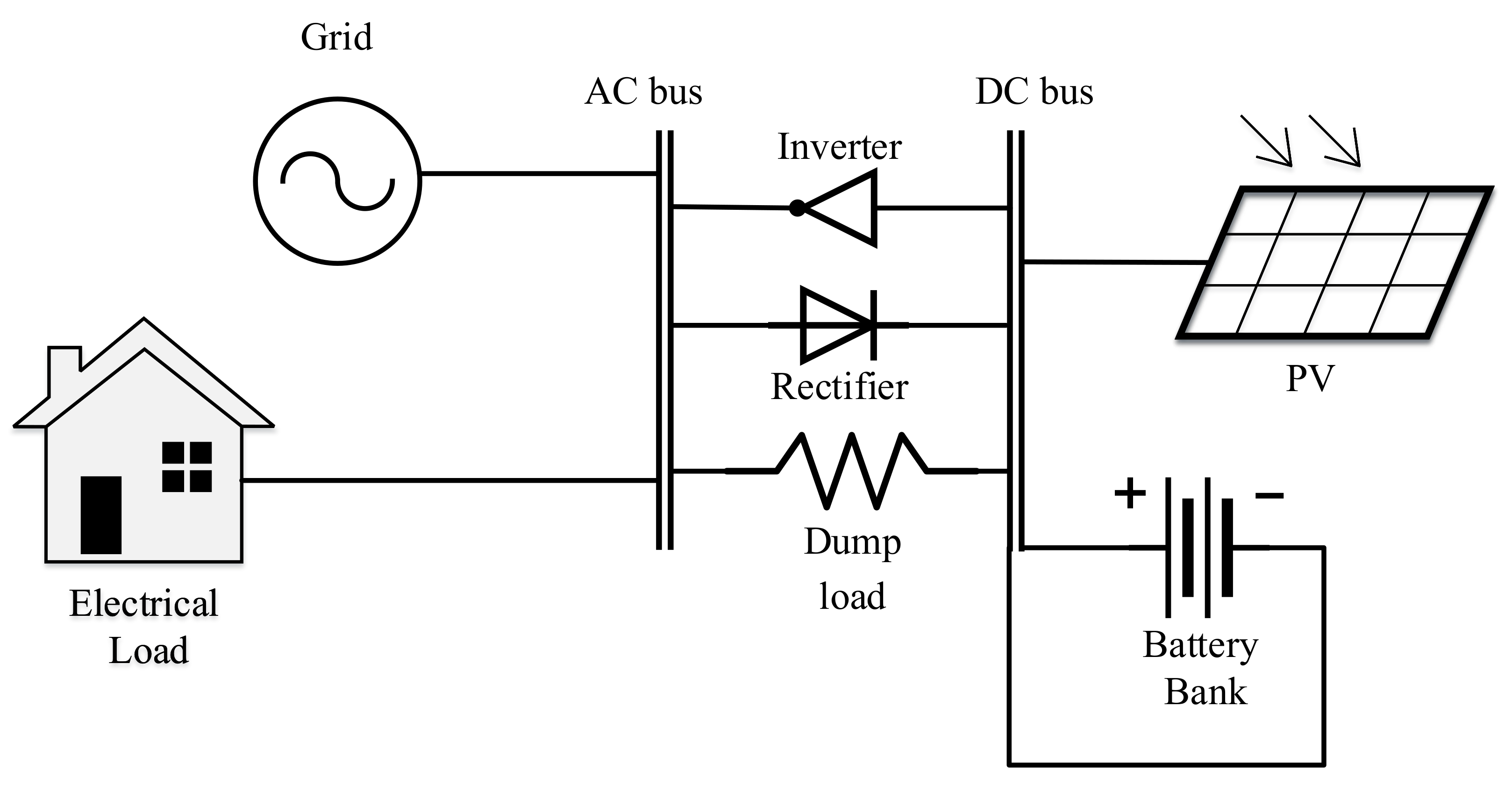
2.2. System Architecture

Figure 7 shows the system architecture considered in this study. PV array and battery banks are on the DC bus and are connected to the grid and load via a bi-directional converter with a size large enough to allow for maximum demand to flow between the AC and DC sides of the system. A dump load is a dummy load (such as heat resistor) that can divert excess energy and maintain the energy balance of the system. It is connected from both ends, although in this case, only the DC side will generate excess energy to be dumped since there are no other AC renewables in the system (e.g., no wind turbines).

This architecture is chosen given that PV installation can be on the rooftop of the hospital, where land acquisition, consent, and permitting processes are simpler. Furthermore, the footprint of the battery bank is small and is usually accommodated within the utilities rooms available in the hospital.

2.3. Electrical Power Modelling

2.3.1. PV Array

The electrical power output of the PV array can be calculated from the following equation [25]

$$P_{pv}=A_{pv}{G}_T{\eta }_{pv}\left(1+{\alpha }_p(T_c-T_{c,stc})\right)$$

(3)

where $A_{pv}$ [m${}^2$] is the surface area of the PV modules, $G_T$ [W/m${}^2$] is the global irradiance incident on the plane of the PV module, ${\eta }_{pv}$ is the system efficiency; ${\alpha }_p$ [$\%/{\mathrm{C}}^{\mathrm{o}}$] is the module’s temperature derating coefficient; $T_c$ is the temperature of the cell surface and $T_{c,stc}$ is the temperature of the cell surface at standard test conditions (STC). The last term in Equation (3) takes into account the effect of ambient temperature on the efficiency of the module by introducing the efficiency correction term proportional to the difference in the cell surface temperature between standard test conditions and the prevailing cell temperature on site. The model assumes that maximum power point tracking is included to obtain maximum output at each irradiance level.

2.3.2. Battery Bank

In this study, we consider a single-node storage model to calculate the battery’s State of Charge (SoC) as follows [32,33]

$$SoC\left(t\right)=SoC(t-\mathsf{\Delta }t)(1-\delta )+\frac{(P-L)\times \mathsf{\Delta }T}{N_{bat}{V}_{bat}{A}_{bat}}{\eta }_{bat}$$

(4)

where, $\delta$ is the internal self-discharge rate of the battery; $\mathsf{\Delta }T$ is the interval at which the measurements are taken. In this work, $\mathsf{\Delta }T=1$ hour unless otherwise stated. The term $(P-L)\mathsf{\Delta }T$ is the net energy flow into the battery bank during one hour. The term $P_{bat,nom}=N_{bat}{V}_{bat}{A}_{bat}$ is the nominal capacity of the battery bank and ${\eta }_{bat}$ is the round-trip efficiency of the battery.

At each timestep in calculating the battery’s SoC, two quantities are needed, namely, the extractable power from the battery $P_{bat,e}$ and the electrical power required to fill up the battery $P_{bat,f}$. They are calculated as follows:

$$\begin{array}{c}\hfill P_{bat,e}=\left(So{C}_{max}-So{C}_{t-\mathsf{\Delta }t}\right)P_{bat,nom}\end{array}$$

(5)

$$\begin{array}{c}\hfill P_{bat,f}=\left(So{C}_{t-\mathsf{\Delta }t}-So{C}_{min}\right)P_{bat,nom}\end{array}$$

(6)

2.3.3. Grid Electricity

In this work, the system can interact with the grid in a bi-directional manner. Electricity is imported from the grid to provide the balance of energy, when the PV-battery system cannot cover the load. In times of high generation and low demand, excess electricity can be exported back to the grid. The amount of export is usually capped by the size of the circuit breaker, which in turn is based on the maximum electrical demand of the building. In this study, the hourly exports are capped at $125\%$ of the maximum electrical demand. This is taken as an approximation of the rating of the circuit breaker feeding the wards, given that data about the actual rating were not available. Losses in transmission for imports and exports are neglected.

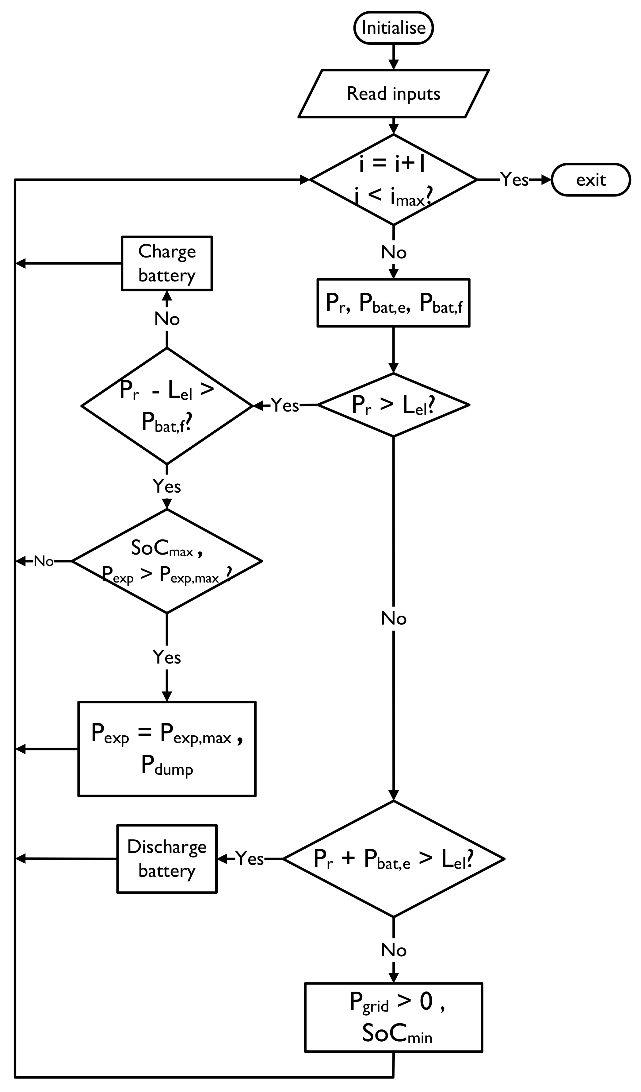
2.4. Dispatch Strategy

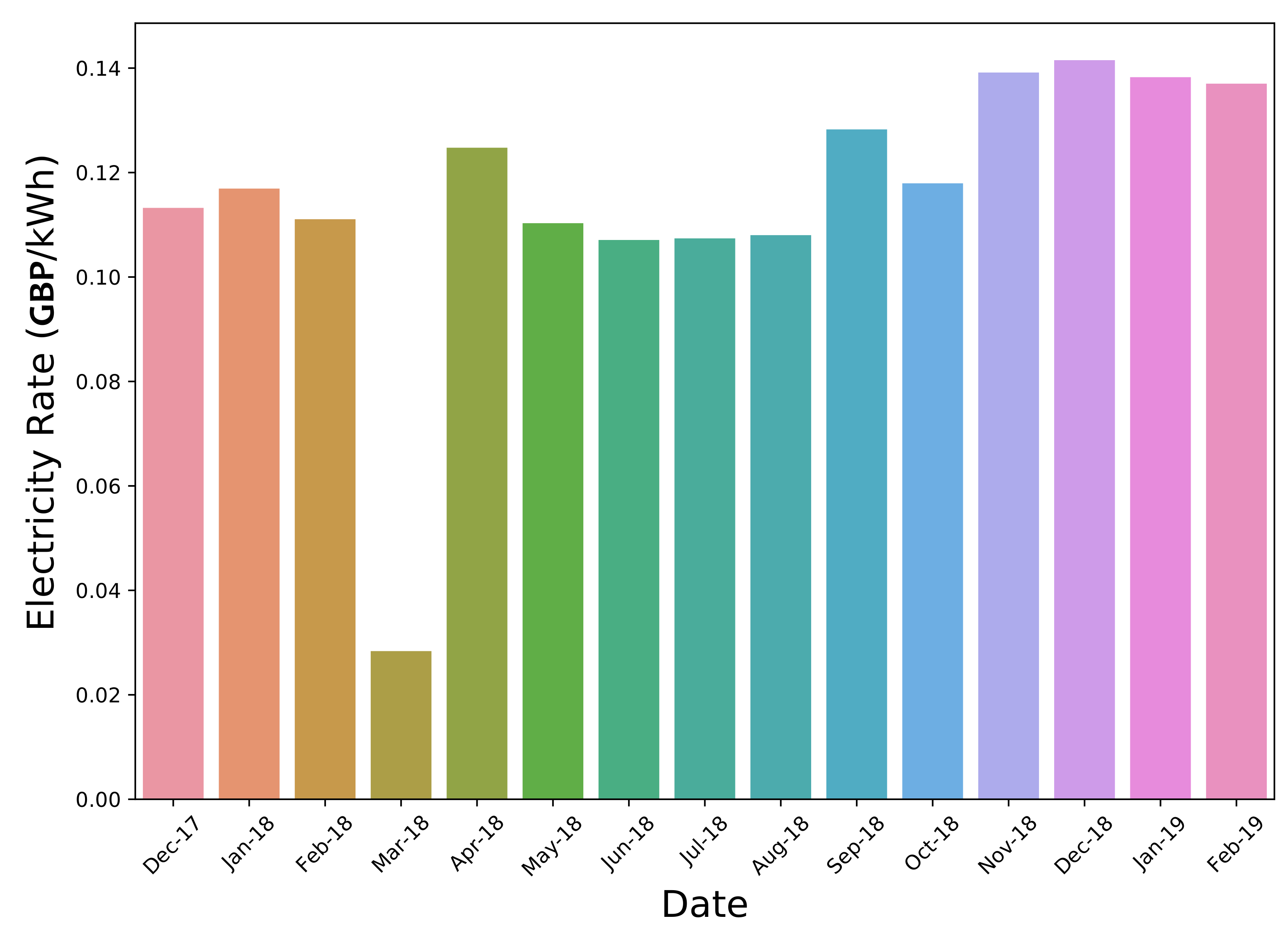
The dispatch strategy is the electrical power management algorithm that controls the balance of energy of the components, most importantly the battery bank. As can be seen in Figure 8, the dispatch strategy used has constant preference of renewable electricity, because PV electrical output is non-dispatchable. Moreover, there is a significant price difference between importing and exporting electricity to the grid (i.e., it is always better to use the local renewable electricity).

When there is excess renewable electricity, the algorithm will check if the energy can be absorbed by the battery, if there is still excess, it will be exported back to the grid. If the battery is full and the export to the grid reached its limit, the rest will be dumped via the heating element. On the other hand, when there is a deficit, the algorithm will check if there is enough charge in the battery to fulfil the demand. If not, then grid electricity is used to cover the deficit. In this case, the battery bank is discharged to the minimum allowable state of charge.

2.5. Cost Modelling

Cost modelling is used to evaluate the cost of the system through its lifetime. The cost components considered in this study are: (i) capital cost; (ii) fixed operation and maintenance cost; (iii) variable operation and maintenance cost; (iv) replacement cost; and (v) salvage costs. For each system component, the discounted cost over the entire life project is calculated and summed to give the total net present value $C_{NPC,tot}$. The discounted cost is calculated from the nominal cash flow using a discount factor, which is determined as [6,34]

$$f_d=\frac{1}{{(1+i)}^N}$$

(7)

where, N is the total project life (in years) and i is the real discount rate, which can be calculated from the expected inflation rate

$$i=\frac{i^{\prime }-f}{1+f}$$

(8)

where, $i^{\prime }$ is the nominal discount rate. $C_{NPC,tot}$ is then used to calculate the total annualised cost (total discounted cost split equally over the entire project years) as follows:

$$C_{ann,tot}=CFR\times C_{NPC,tot}$$

(9)

where, CFR is the capital recovery factor, which can be calculated as follows [35]

$$CRF=\frac{i{(1+i)}^N}{{(1+i)}^N-1}$$

(10)

Finally the Levelised Cost of Energy (LCE) can be calculated as follows [35,36]:

$$LCE=\frac{C_{ann,tot}}{P_{tot}-P_{dump}}$$

(11)

where, the value in the denominator represents the useful electrical energy. It is the sum of the renewable and grid electricity minus the dumped energy, which does not add value to the system.

2.5.1. Cost Parameters of System Components

Accurate cost parameters are crucial in obtaining representative results. As shown in [6], the prices of renewable energy components have seen a steep decline over the past decade and this trend continues to the present. The most up-to-date values for the UK market are compiled and adapted from [5,37] after taking a $0.73$ conversion ratio between USD and GBP.

PV array: the total installed cost of a residential PV system is around GBP 1600/kWp, and for commercial PV systems, it is GBP 1125/kWp. We will assume a median price of GBP 1350/kWp.

Battery bank: getting an accurate estimate of the installed cost of battery bank is more challenging, given that sizing methodologies assumes a certain size of the system in order to perform cost calculations and projections. However, it is clear that the cost of storage is declining rapidly and is projected to continue the decline in the next decade in the range of $30\to 60\%$ [37]. According to the latest figures from [5], the UK’s median price for Lithium ion battery bank for stationary applications is around GBP 545/kWh of net capacity (the usable capacity $(So{C}_{max}-So{c}_{min})\times P_{bat,max}$). On the other hand, the authors in [37] put the cost around GBP 255/kWh for a 4-h utility scale system. This does not include installation costs. The lifetime of the batteries also varies between 10 and 20 years. From the above discussion, we chose to account for GBP 545/kWh as the total installed cost for the battery bank.

Grid: The cost of grid-electricity is taken according to Figure 3 on a monthly basis. As for the exports back to the grid, given that, at the time of the study there was no PV system, actual data are not available. In this study, an average export tariff of GBP 0.04/kWh was adopted.

The values of the cost parameters used in this study are summarised in

Table 1. Cost Parameters for system components.

Component	Capital	Installation	Fixed	Variable	Replacement	Exports/Salvage	Component Life
	Cost (CC)	Cost (IC)	O&M	O&M	Cost
PV	GBP 50/m${}^2$	2.5 × CC	GBP 2/m${}^2$	0	(CC + IC)	0	25 min
Battery	GBP 300/kWh	0.5 × CC	0.01 × CC	0	(CC + IC)	Linear	(15 years, 3000 cycles)
Grid	0	0	0	variable	0	GBP 0.04/kWh	25

. The total installed cost is divided into capital and installation costs. The cost of the PV module is shown in GBP/m${}^2$ with assumed conversion factor of 8 (1 kWp = 8 m${}^2$).

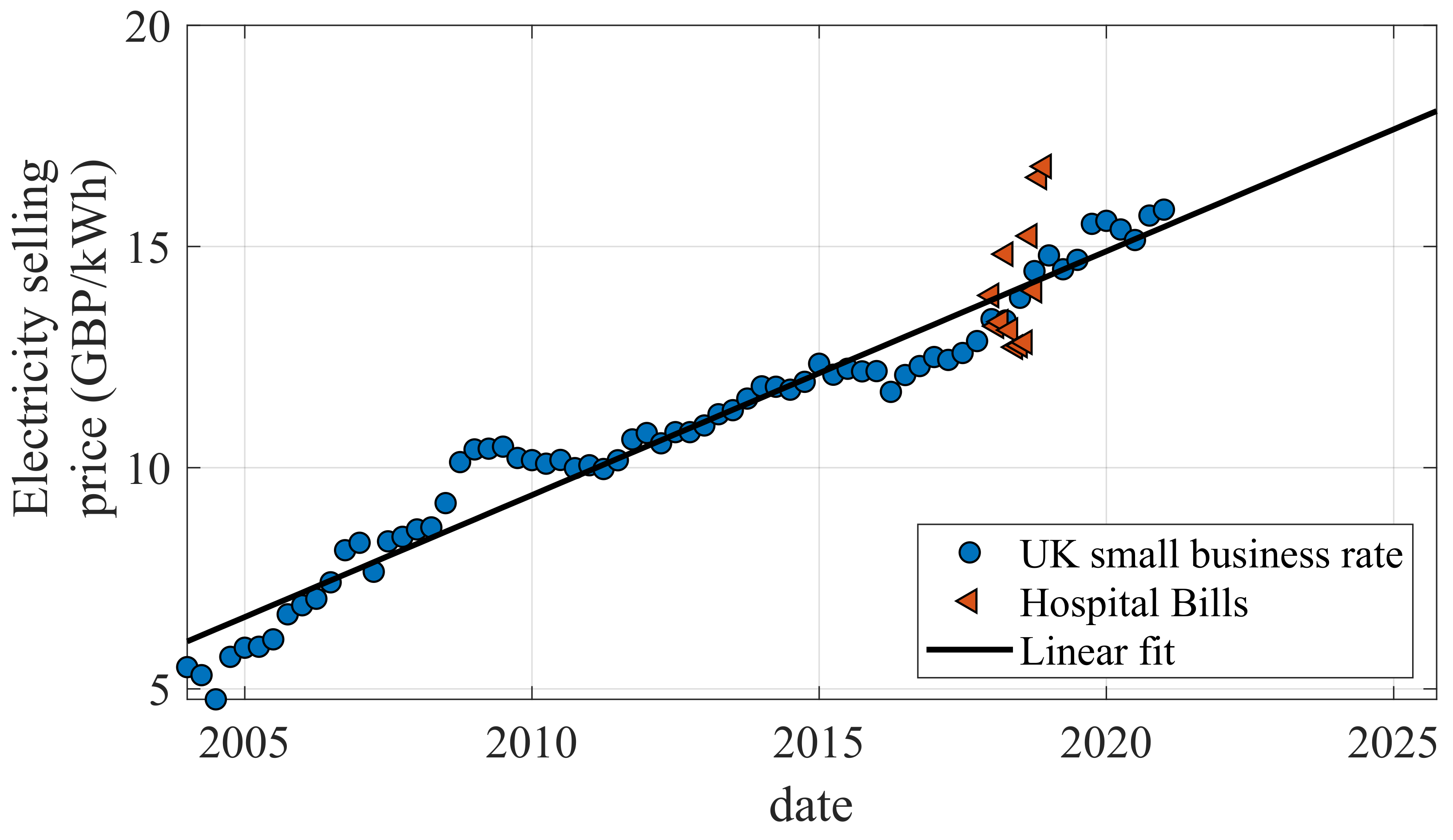
2.5.2. Forecasted Cost Parameters

The most important cost parameters are forecasted and used in the future optimisation of the system, this includes: (i) grid price; (ii) PV module capital cost; and (iii) battery bank capital cost.

Grid:Figure 9 shows the long term electricity selling price in the UK; these prices include the climate change levy and VAT and are taken from [38]. The upward trend is clear; as such, linear fit regression was used to project likely electricity costs in the future. The fit equation is given as:

$$y=0.1378x+5.935$$

(12)

From the above equation, prices of Q3-2023 and Q3-2025 are calculated as GBP 16.82/kWh and GBP 17.92/kWh, respectively.

As for the export price levels, in January 2020, the UK government discontinued the Feed-in-Tariff (FiT) scheme and replaced it with the Smart Export Guarantee Scheme [39]. Under this scheme, only exports are compensated (as opposed to generation and exports in FiT). Individual electricity suppliers will set up their rates. Current rates on offer range from GBp 1.5/kWh to GBp 6/kWh. Customers will be allowed to change suppliers, as such, it was assumed that the average rate of GBp 4/kWh is maintained through 2025.

PV: according to a recent study [40], PV prices are also expected to keep declining. Accordingly, the projected capital cost of PV modules in 2023 and 2025 are $88.4\%$ and $80.7\%$ respectively. These values will be used in scaling the capital cost of the PV modules when conducting the optimisation.

Battery bank: as shown in [37], steep declines in battery costs are projected in the coming years. Here we used the normalised curve to predict the possible price fall in 2023 and 2025, taking the middle of the year as a chosen point of reference. The capital cost price is expected to fall to $79.2\%$ in 2023 and to $68.9\%$ in 2025. These values will be used to scale down the battery price.

Demand: as for the demand, given the lack of long term data to project future consumption, we will assumed constant electrical demand.

2.6. Multi-Objective Optimisation

The decision variables of the study are the main size parameters of the system components. This is mainly the area of the PV array ($A_{pv}$) and the number of batteries $N_{bat}$. A multi-objective optimisation is carried out using genetic algorithm (GA) code developed in MATLAB. The code utilises the built-in GA optimiser. The two objectives to be minimised are LCE and emissions.

$$min\left(LCE(A_{pv},N_{bat}),E_{c{o}_2}(A_{pv},N_{bat})\right)$$

(13)

Reliability constraints were not imposed on the system since it is assumed that the grid electricity is reliable; therefore, no blackouts are expected.

The upper bound of the variables are taken as follows

$$U{B}_{pv}={\alpha }_{pv}\frac{max\left(L_{el}\left(t\right)\right)}{{\eta }_{pv}\overline{G_T}\left(t\right)}$$

(14)

$$U{B}_{bat}=\frac{\beta {\sum }_i^{24}{L}_{el,i}\left(t\right)}{V_{bat}{C}_{bat}}$$

(15)

where ${\alpha }_{pv}=1.1$ is a capacity reserve factor and $\beta =1$ is the autonomy days of the system. $U{B}_{pv}$ is capped at the maximum area at the hospital roof that can be utilised to install PV array. The lower bounds of the variables are set to zero for both to enable the system to eliminate the non-feasible components.

$$\{L{B}_{pv},L{B}_{bat}\}=\{0,0\}$$

(16)

The main GA parameters used throughout the study are shown in

Table 2. Main GA Parameters.

GA Parameters	Value
Population size	200
Max number of generations	400
Probability of crossover	0.8
Convergence criteria	$1\times {10}^{-4}$
Max number of stalled generations	30
Pareto fraction	50%
Number of genes	2
Type of genes	integers
$\{U{B}_{pv},U{B}_{bat}\}$	$\{470,700\}$
$\{L{B}_{pv},L{B}_{bat}\}$	$\{0,0\}$

. The Pareto fraction refers to the proportion of the population on the Pareto front that will propagate to the next generation. Values less than 100% ensure that the population is diverse even if some of the solutions have sub-optimal fitness, which in turn improves convergence to the global optimum. The optimisation run converges if the change in the spread of the Pareto solutions is less than the convergence criteria sustained over the maximum number of stalled generations.

Optimisation Methodology

Optimisation simulations are carried out three times. The first time involves using the prevailing parameters at the present including current cost parameters and grid emissions. Then two further optimisations are carried out for the future state of the system. The first point chosen is mid-2023 and the second is mid-2025. In this way, an informed decision can be reached in which optimum solutions are likely to remain optimum in the future.

3. Results and Discussion

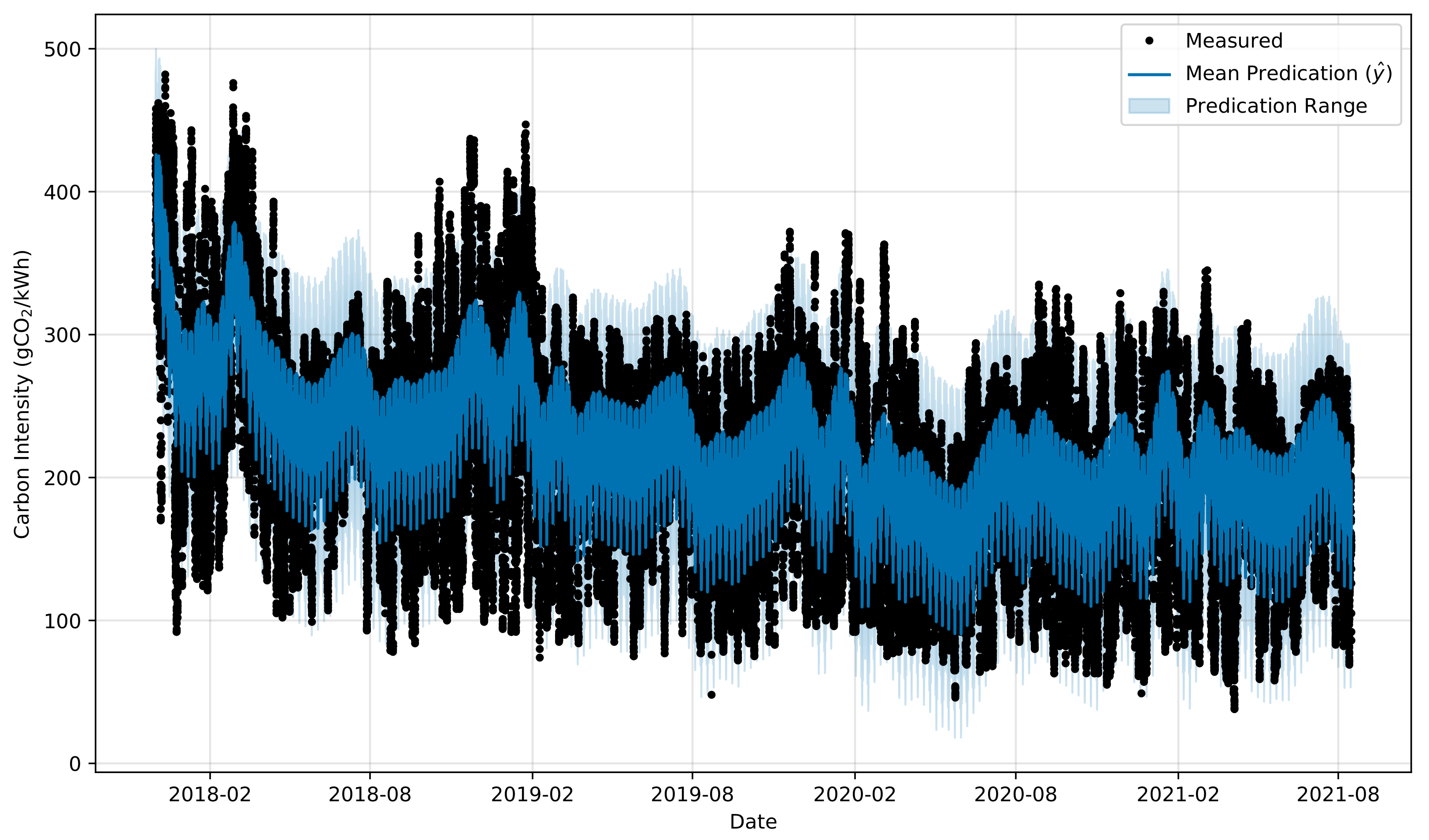
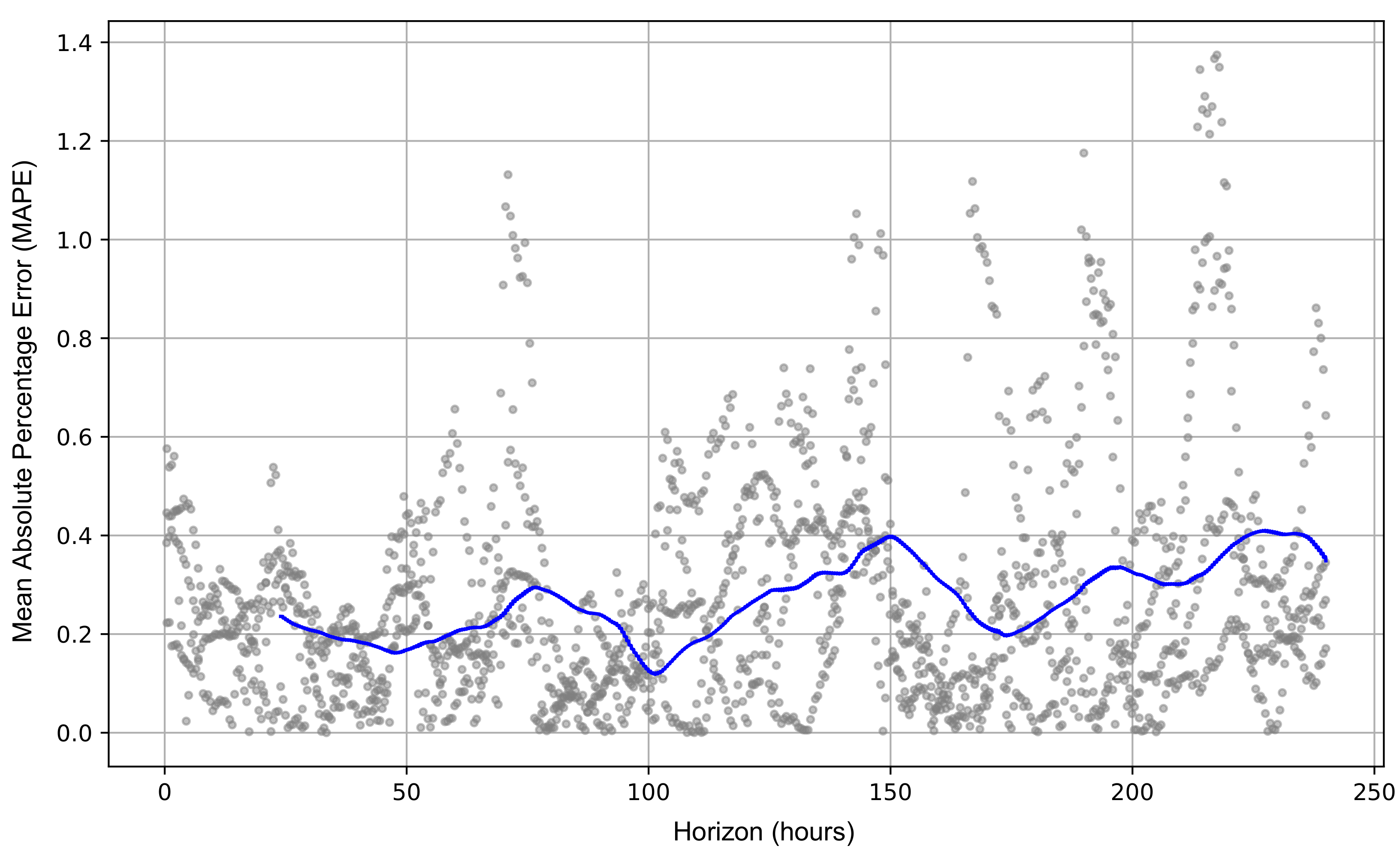
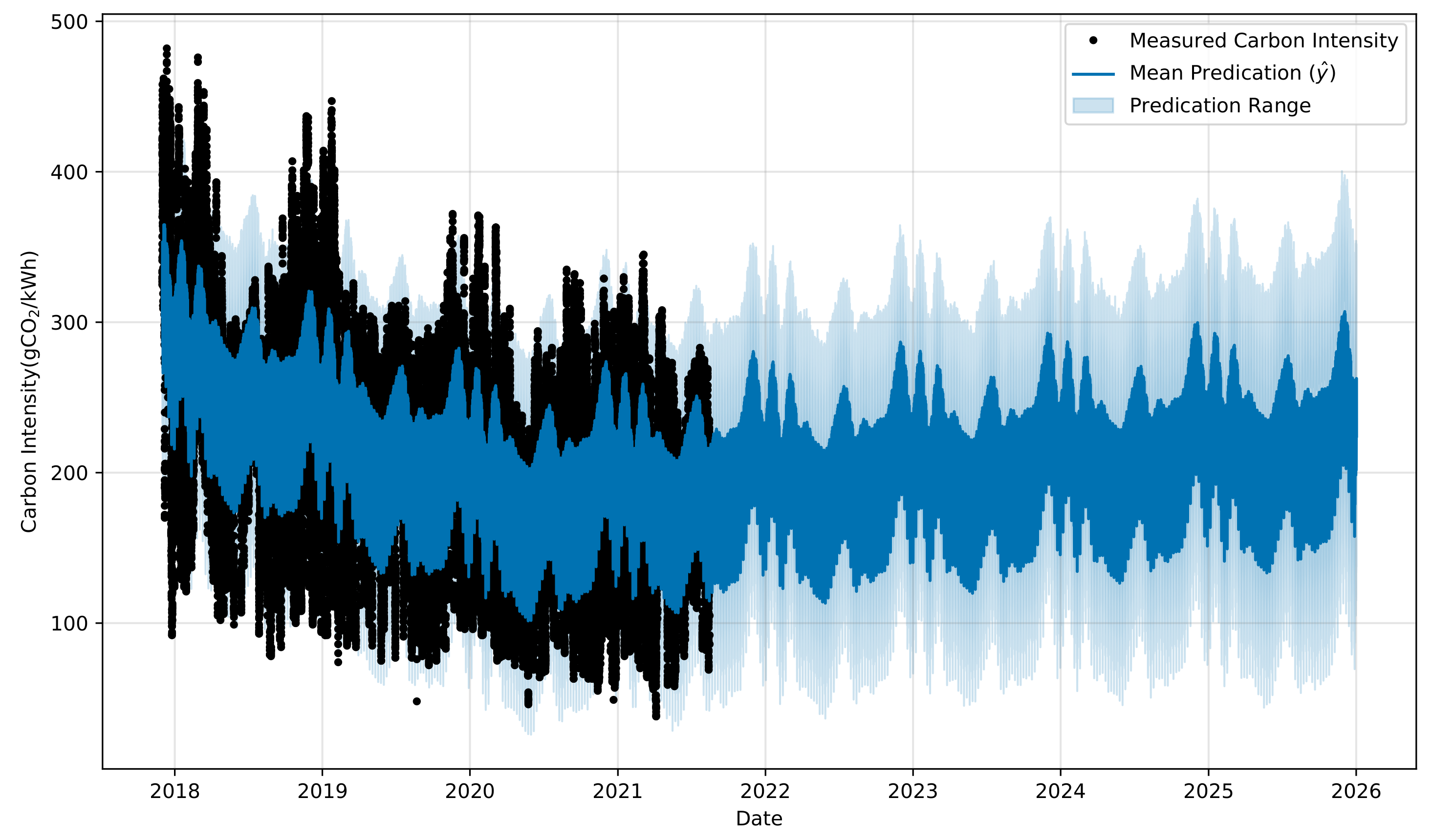
3.1. Grid Carbon Intensity Forecasting

Initially the forecasting model was used and tuned to model the carbon intensity. Figure 10 show the measured values—provided by the dataset—and the forested values ($\widehat{y}$) estimated using the forecasting model. Moreover, we provided the upper and lower limits of the forested values. It can be observed that the model is able to capture the trend; however, some of the outliers and the sudden changes in the values are not captured in the model. The accuracy of the model is assisted by using the mean absolute percentage error (MAPE). As shown in Figure 11, the model achieves very low errors, in particular, the MAPE ranges between 0.1 and 0.5.

Thus, the model was used to forecast the carbon intensity for the period between August 2021 and December 2025. As shown in Figure 12, the range carbon intensity would remain as it is at the moment, since in the model, we are not assuming any change in the grid or the electricity generators. The predication mean values were utilised in Section 3.3 to evaluate the performance of the optimised systems.

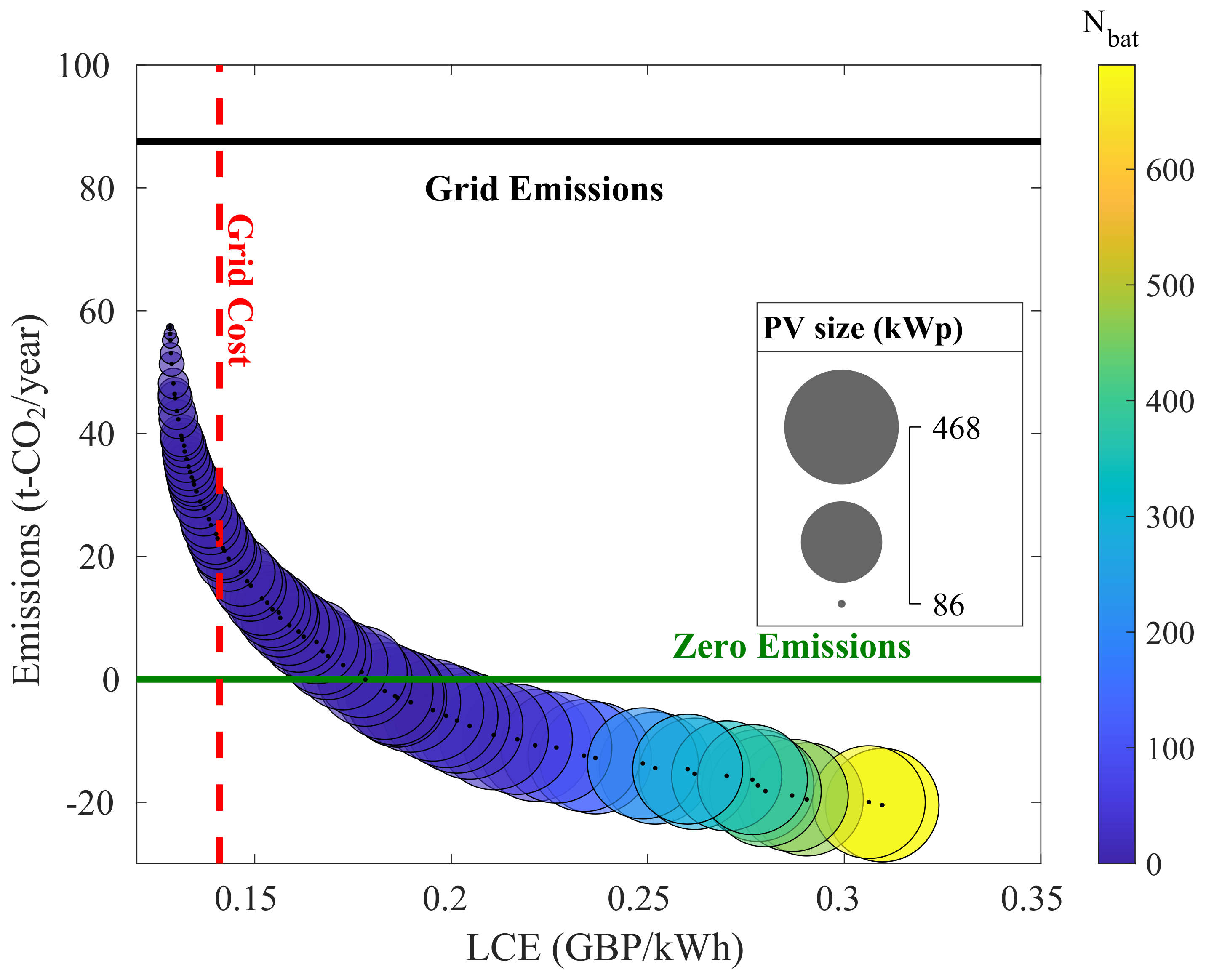
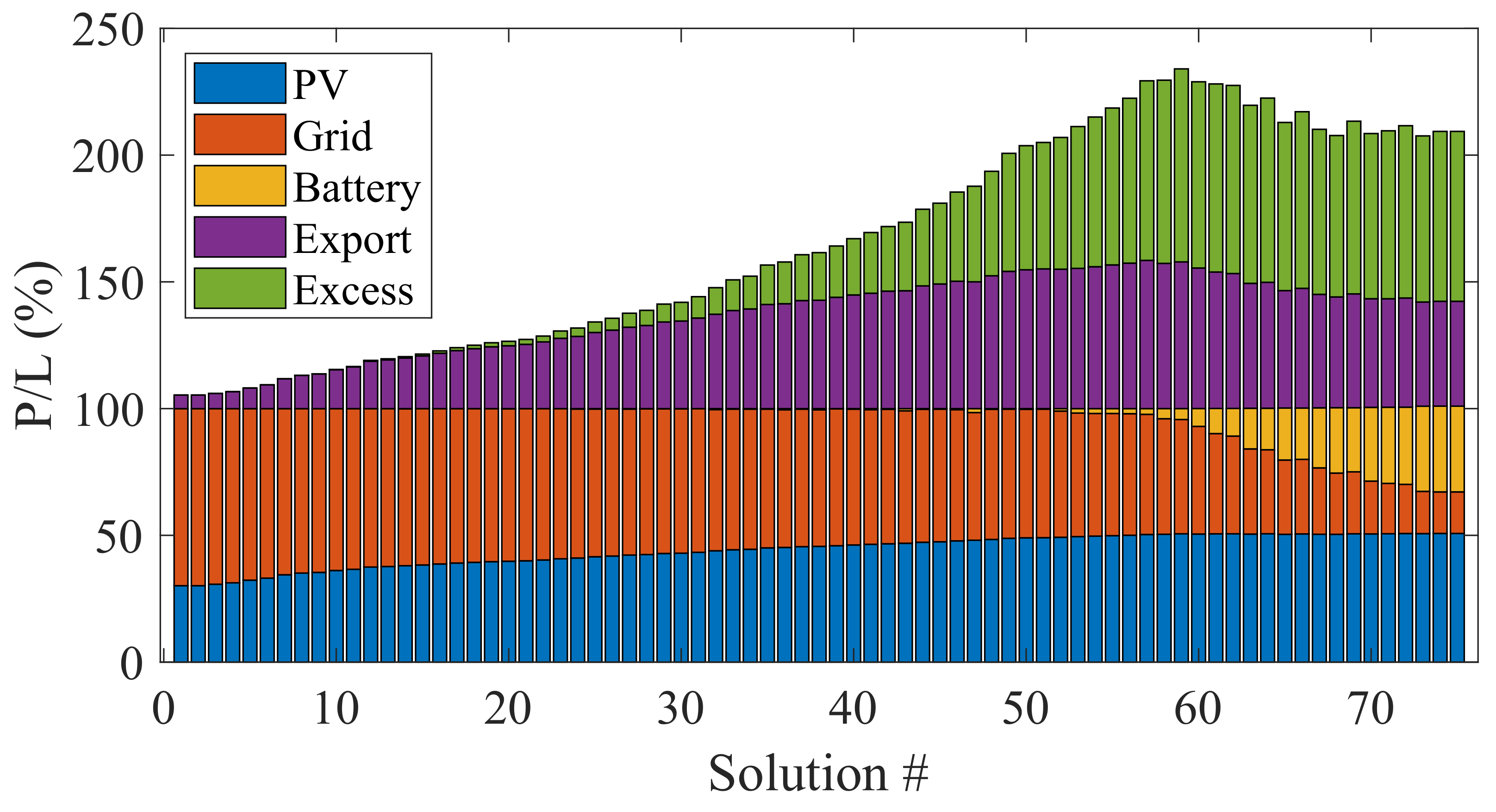
3.2. Optimum PV-Battery System

Figure 13 shows the Pareto front in objective function space. The size of the bubbles represent the PV system size and the colour represent the number of batteries. Baseline grid emissions and cost are shown for comparison, as well as the zero emissions level. Solutions to the left of the grid-cost line (red-dotted line) are solutions with lower cost than existing grid-only system. Solutions to the right of the red line and over the green line are solutions that are more expensive but with lower emissions. Solutions under the green line will have overall negative emissions because of the large amount of export back to the grid. All the solutions that have more than zero emissions have no or small number of batteries.

Table 3. Sorted Pareto front solutions, solutions 1–28 are cheaper than existing grid, solutions 29–47 have deeper emission reductions, approaching net zero, solutions 48 to 74 have net negative emissions.

Sol	LCE	${\mathit{E}}_{{\mathbf{co}}_2}$	${\mathit{P}}_{\mathbf{pv}}$	${\mathit{N}}_{\mathbf{bat}}$	Sol	LCE	${\mathit{E}}_{{\mathbf{co}}_2}$	${\mathit{P}}_{\mathbf{pv}}$	${\mathit{N}}_{\mathbf{bat}}$
#	(GBP/kWh)	(t/year)	(kWp)	(#)	#	(GBP/kWh)	(t/year)	(kWp)	(#)
1	0.1285	57.3	86	0	38	0.1565	10.0	267	1
2	0.1285	56.3	89	0	39	0.1588	8.8	275	2
3	0.1285	55.2	92	0	40	0.1612	7.8	282	4
4	0.1287	53.1	98	0	41	0.1625	6.9	288	3
5	0.1289	51.3	103	0	42	0.1657	6.1	294	9
6	0.1293	48.2	112	0	43	0.1673	4.5	306	3
7	0.1296	46.4	117	0	44	0.1686	3.8	312	2
8	0.1298	45.7	119	0	45	0.1725	2.3	324	4
9	0.1302	43.7	125	0	46	0.1772	1.2	333	17
10	0.1306	42.3	129	0	47	0.1782	0.0	345	3
11	0.1313	39.7	137	0	48	0.1831	−1.9	363	2
12	0.1315	39.0	139	0	49	0.1857	−2.7	371	3
13	0.1321	38.0	142	1	50	0.1863	−3.0	374	2
14	0.1322	37.1	145	0	51	0.1897	−3.7	381	10
15	0.1327	35.8	149	0	52	0.1953	−5.0	394	19
16	0.1332	34.6	153	0	53	0.1987	−5.9	404	21
17	0.1336	33.7	156	0	54	0.2014	−6.7	413	21
18	0.1340	32.9	159	0	55	0.2047	−7.6	423	22
19	0.1345	32.3	161	1	56	0.2108	−9.1	441	25
20	0.1346	31.7	163	0	57	0.2168	−9.8	446	47
21	0.1352	30.6	167	0	58	0.2213	−10.8	458	51
22	0.1361	28.9	173	0	59	0.2267	−11.1	452	87
23	0.1372	27.9	177	2	60	0.2338	−12.4	457	126
24	0.1384	26.1	184	2	61	0.2367	−12.8	458	140
25	0.1389	25.1	188	1	62	0.2488	−13.7	451	215
26	0.1402	23.7	194	2	63	0.2519	−14.5	459	219
27	0.1405	23.0	197	1	64	0.2601	−14.6	445	284
28	0.1419	21.4	204	1	65	0.2619	−15.4	455	278
29	0.1423	20.9	206	1	66	0.2701	−15.7	446	334
30	0.1434	19.7	212	0	67	0.2766	−16.3	445	369
31	0.1465	17.5	223	4	68	0.2780	−17.3	458	357
32	0.1481	16.0	231	2	69	0.2799	−18.2	455	435
33	0.1490	15.2	235	2	70	0.2867	−18.9	460	462
34	0.1519	13.2	247	2	71	0.2904	−19.5	466	472
35	0.1532	12.5	251	5	72	0.3063	−20.0	463	679
36	0.1545	11.4	258	2	73	0.3096	−20.5	468	690
37	0.1561	10.9	261	5	74	0.3096	−20.5	468	690

shows the sorted solutions at the Pareto front with corresponding fitness and system size values.

As can be seen from Figure 14, the share of each of the electrical supply components is shown as a ratio of the total electrical demand. PV, grid, and battery components make up 100% of the demand. The direct PV contribution ranges between 30% for solution 1 and 50% for solution 74. Exports to the grid steadily increase until the size of storage becomes bigger than 50 kWh then the ratio starts declining. Excess energy becomes significant between solutions 25 and 74. This is mainly due to the large increase in PV output in the warm part of the year, while the exports are limited as discussed in Section 2.4. The high levels of excess is mostly responsible for increasing the overall cost of the system as this excess energy is not considered useful and do not contribute to the revenue.

Further assessment of the optimum solutions is shown in Figure 15. In Figure 15a, payback period is calculated for all the solutions. It is an important metric to measure the economic viability of a project. The simple payback is the number of years to reach the break-even point; where the cumulative savings have equalled the initial investment [41]. A system is deemed profitable when the payback period is smaller than the project life. It can be seen that solutions $1\to 45$ can be considered profitable with payback period from approx 8 years for solution 1 to 24.8 years for solution 45. In Figure 15b the cumulative savings are calculated by subtracting the total initial expenditure from the yearly savings until the end of the project [42]. As can be seen, systems that have a payback period of less than the project life will generate revenue (solutions $1\to 45$ with maximum savings for solution 1 of around GBP $270,000$.

Similarly, Figure 15c shows the cumulative ${\mathrm{CO}}_2$ savings in tonnes. The calculations assumed constant ${\mathrm{CO}}_2$ emissions from the grid throughout the lifetime of the project. Values ranged from around 800 tonnes for solution 1 to around 2800 tonnes for solution 74.

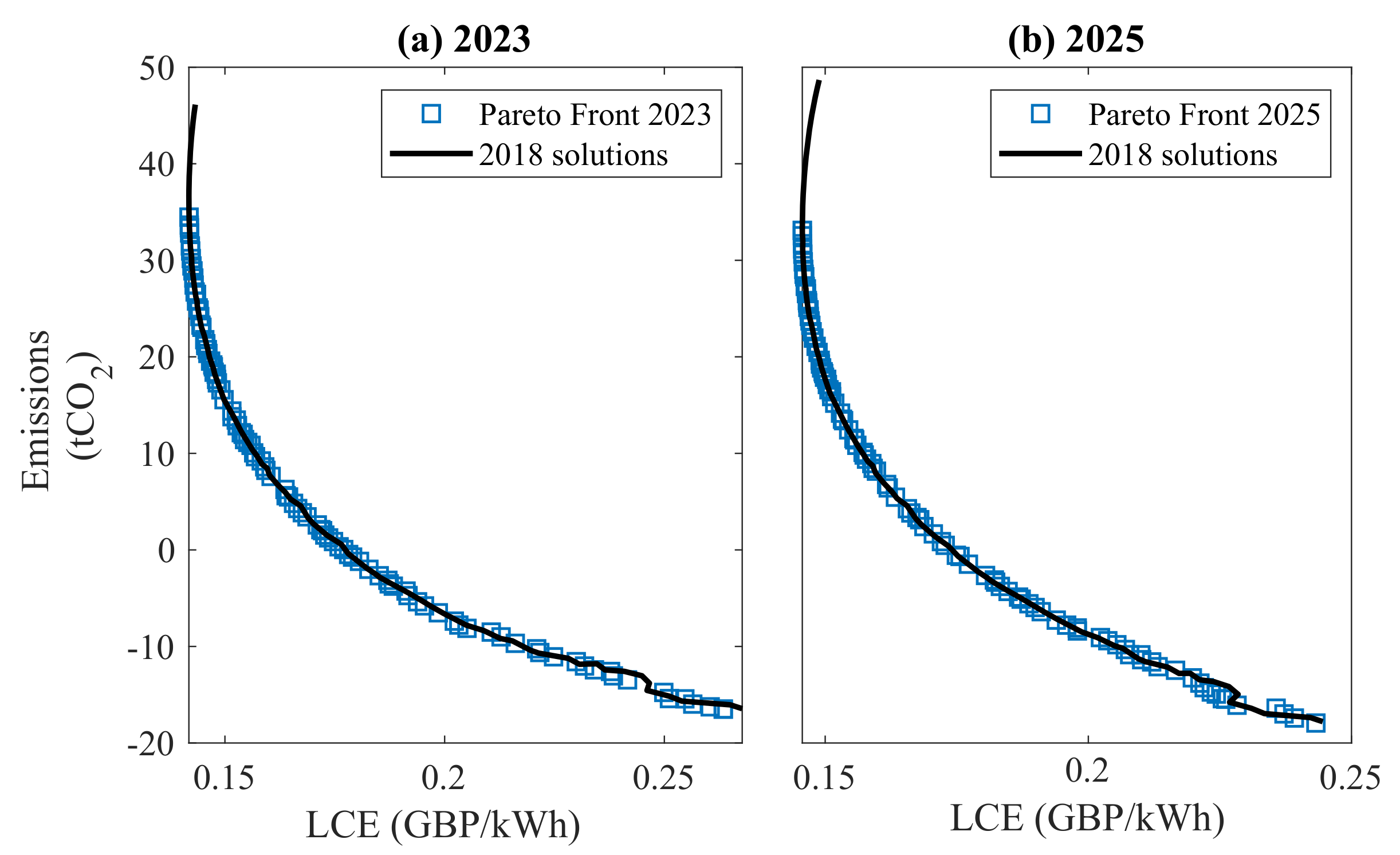
3.3. Optimisation Using Forecasting Data

In this section, we perform optimisation of the system using forecasted emissions, grid-prices, PV, and battery capital costs in years 2023 and 2025. The original solutions will be referred to as solution 2018 given that the electrical consumption data were taken in 2018.

Figure 16 shows the optimisation results using the parameters from Table 1 and then projected parameters for 2023 and 2025 including PV capital cost, battery capital cost, forecasted emissions, and grid prices. The 2018 Pareto front produced the most cost competitive results in absolute terms, especially in the region of high emissions(top left). This can be attributed to the lower prevailing grid prices, which constitutes around $60\%$ of the supply share. On the other hand, in 2023 and 2025, a larger proportion of the Pareto solution is situated to the left of the baseline cost (grid only system). The difference between the cheapest solution in 2018 and the grid-only cost is GBP 0.01201/kWh, this increased to GBP 0.026358/kWh in 2023 and to GBP 0.033547/kWh in 2025. Furthermore, in 2025, it would be possible to reach a net zero system while being cheaper than the grid. The size of the system in 2023 and 2025 solutions was consistent with the 2018 solution, whereby most of the solutions have little storage capacity until PV system becomes larger than 400 kWp nominal power. This indicates that the optimum configuration is unlikely to change in the future, rather, the overall cost of the system will change depending on the change in the financial parameters as shown in Figure 16.

The optimum solutions of 2018 are evaluated using the forecasted parameters of 2023 and 2025 and compared with the Pareto solutions of the respective years are shown in Figure 17. This comparison enables us to estimate how the optimum solution chosen based on 2018 parameters would change in the future. It can be seen that optimum solutions in 2018 remain on or very close to the Pareto solutions in 2023 and 2025. However, the cheapest solutions in 2018 (solutions # 1 to 12) are out of the Pareto solutions. This indicates that, if the projections are accurate, the solutions will no longer be optimal in the future and, therefore, should be avoided.

Figure 18 shows how the payback period changes when forecasted parameters are used to estimate payback of the original Pareto solutions (refer to Figure 13). It can be seen that the payback period is expected to accelerate driven by the combined effect of reductions in PV and battery prices and the expected increases in the grid prices. The cheapest solution will have a reduction of payback by around 2.5–3 years. Furthermore, all the optimum solutions will become commercially viable by having payback less than the project life, including solutions with net negative emissions.

Figure 19 shows a method to recommend a subset of the Pareto front solutions based on the projected optimisation values. The plot is for LCE against the corresponding size of the PV system. The Pareto fronts for 2018, 2023, and 2025 are shown. The bottom horizontal line shows the minimum PV size on the Pareto 2025 solutions. The upper horizontal line shows the zero emissions line (above which are negative emission solutions). The two vertical lines are the grid-prices in 2018 and 2025. The two vertical and horizontal lines define several regions in the plot. Area 1 shows the optimum solutions in 2018 that will become sub-optimal in the future. This can be observed from the 2023 and 2025 solutions that will undergo change in direction. This is due to the relatively large grid-import proportion of the total supply share, combined with increase in the grid electricity price. Area 2 contains solutions that will remain at optimal in the future and are still cheaper than the existing grid-only system. However, these solutions will also get significantly more expensive in the future as the cost of the grid increases. In area 3, solutions will remain optimal and will undergo small increase in the future. Solutions in area 3 are more expensive than the current grid-only system but will become cheaper in the future. Furthermore, these solutions will have smaller ${\mathrm{CO}}_2$ footprint by comparison with solutions in areas 1 and 2.

As such, it can be concluded that solutions in areas 2 and 3 are the most suitable and the choice of which area is more preferable will be according to the preferences of the client. Referring back to Table 3, solutions $1\to 12$ fall in area 1. Solutions $13\to 26$ are in area 2 and solutions $27\to 47$ are in area 3.

4. Discussion of the Results

It can be seen from the optimisation results that installing PV system with 30–40% share will be economically viable, while at the same time, decreasing the carbon emissions from the hospital by 800–1000 tonnes of ${\mathrm{CO}}_2$ over the lifetime of the PV array. Increasing costs of the grid plays a major role in shifting the optimum solutions towards larger PV installation and possibly introducing storage to complement the production and reduce exports back to the grid. The elimination of the battery bank from most of the optimum solutions can be attributed to the good match between demand and irradiance (refer to Figure 6) combined with the high capital cost of batteries. We carried out optimisation simulations using capital cost of batteries less than GBP 200/kWh, the optimum solutions contained significantly larger battery banks. This indicates that, in the near future, grid-PV-battery architectures will become optimal.

Given the large amount of excess energy that cannot be exported back to the grid, it would be beneficial to reduce this amount by either increasing the levels of storage or by utilising in the heating and cooling of the hospital. This seems like a good opportunity to utilise the excess energy generated on site in fulfilling dispatchable loads such as heating, cooling and ventilation.

5. Conclusions

In this study, we investigated supplying a healthcare facility in the south-east of England with a grid-connected HRES. Multi-objective optimisation with cost and emissions as objectives was performed using prevailing prices and projections of emissions and costs for 2023 and 2025. Taking the future state into consideration, a subset of the optimal solutions can be recommended based on the preferences of the end-user. The following conclusions can be drawn:

-

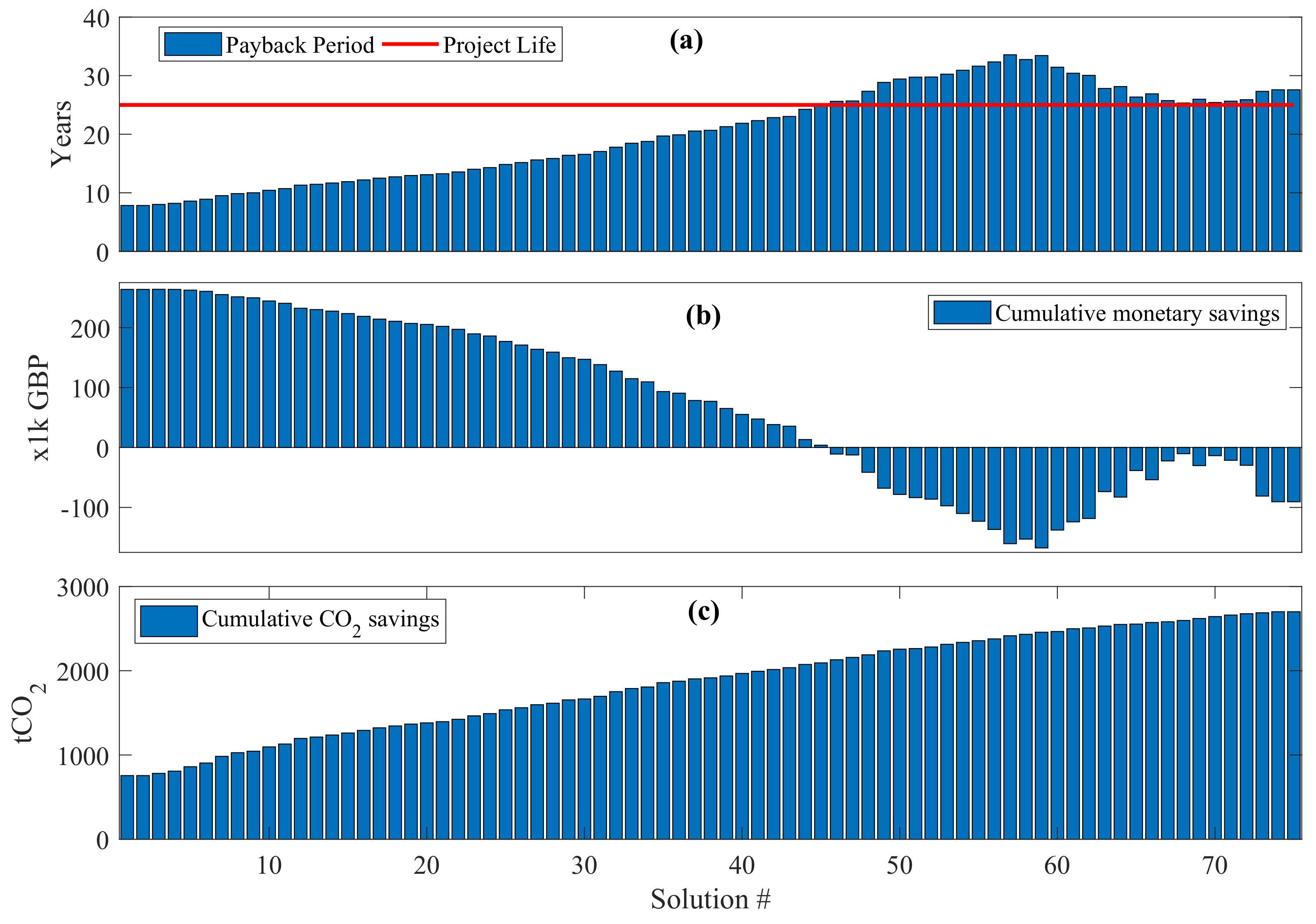
In the UK healthcare context, installing grid-connected HRES can be economically viable and can even help reduce the cost of energy than grid-only system, yielding cumulative savings in the same order of magnitude as the initial cost over the lifetime of the system. A side benefit includes dampening the effects of grid-price fluctuations on the overall energy cost of the hospital. Given the long term trend of electricity price increase in the UK, the system can become more profitable with time.

-

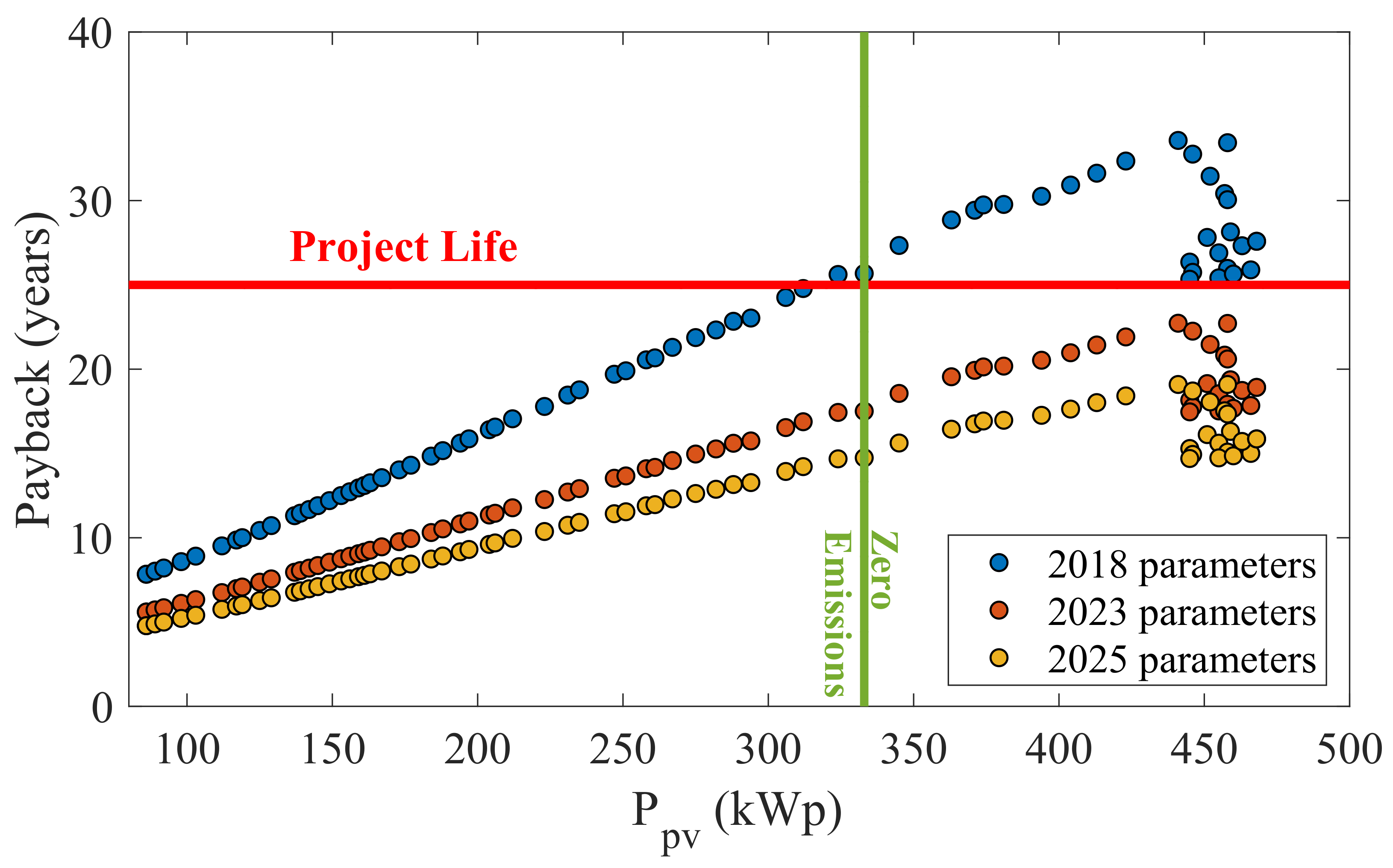
Installing grid-connected HRES will directly address the NHS ambition of becoming net-zero health provider. A Net-zero system for the hospital section under study, will save around 2000 tonnes of ${\mathrm{CO}}_2$ over 25 years of project life.

-

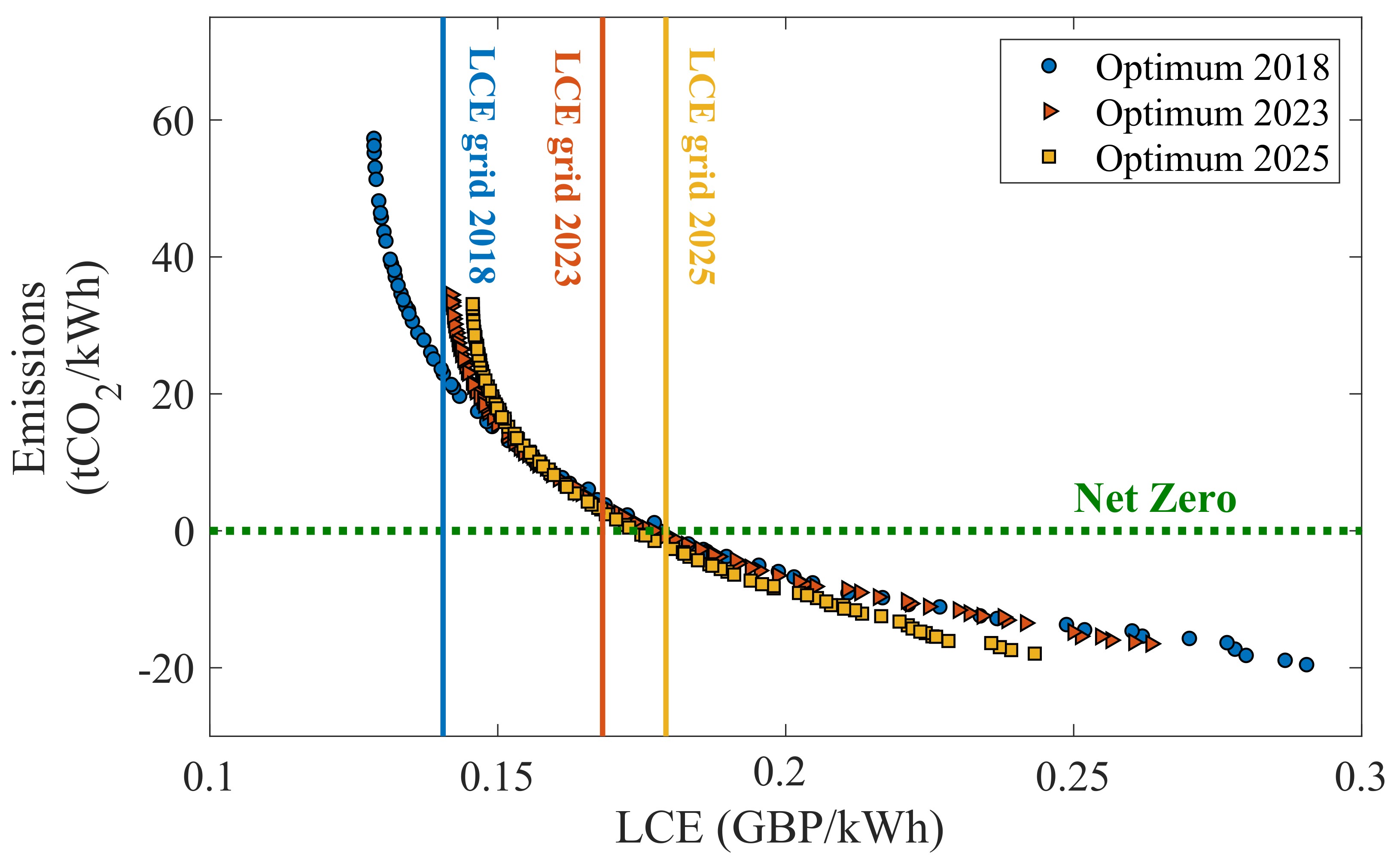
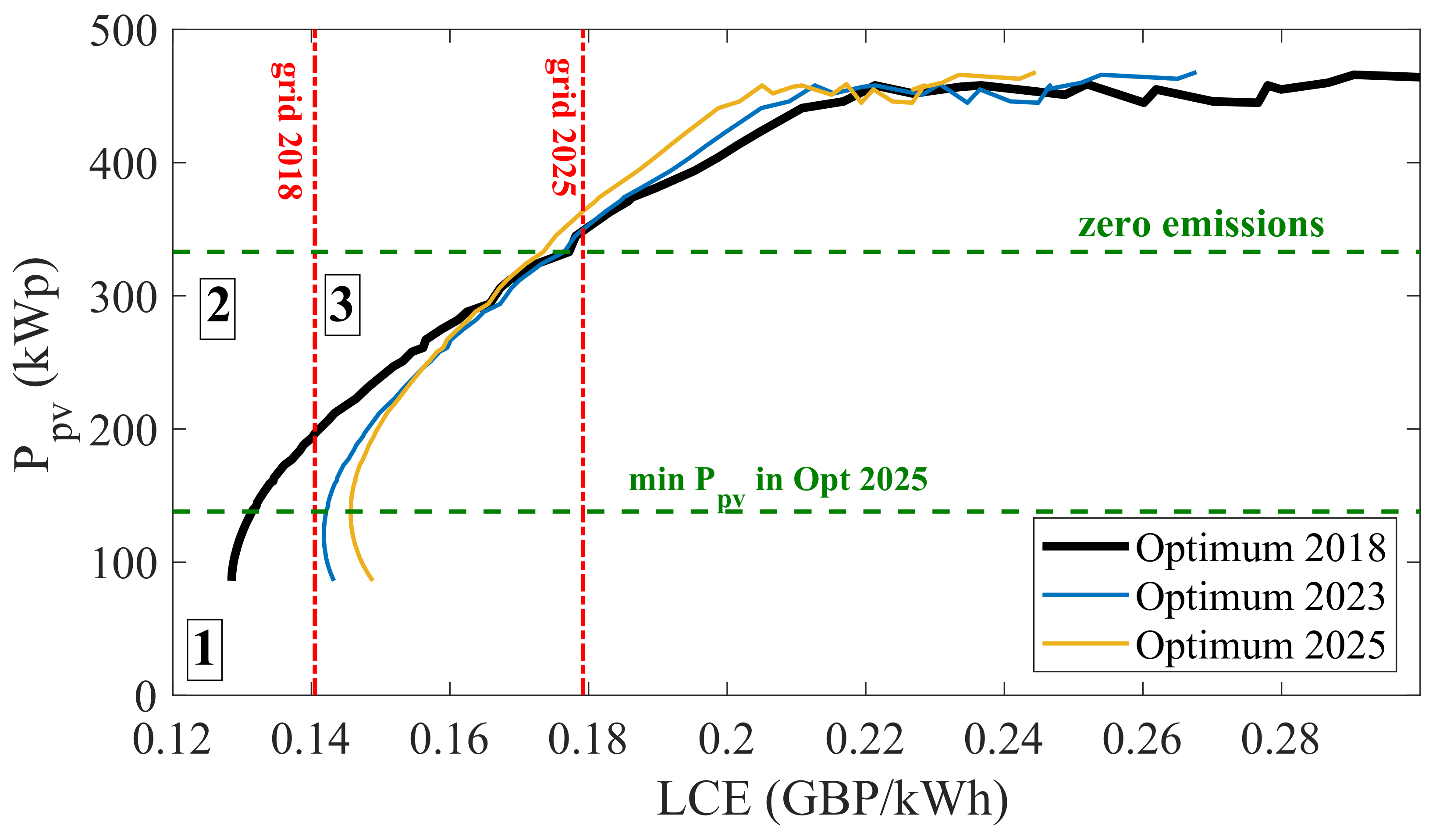
If our projections of grid-emissions and cost parameters are accurate, then the optimum systems will become more cost effective in the future.

-

Incorporating forecasting into the optimisation helped in selection of the most suitable subsets of the Pareto solutions, which was not obvious without using this approach.

-

A significant drop in storage prices or a change in the exports to the grid mechanisms are needed to make the grid-PV-battery system the optimal choice. Significant reductions in battery prices are expected over the coming years and changes to export incentives by offering higher rates for customers with storage are starting to emerge in the UK electricity market.

Finally, some further work that is considered for the future include: more extensive use of forecasting from using two points in the future to the entire life of the project. Utilisation of excess energy in the supplying thermal loads and dispatchable loads, and studying more sophisticated HRES structures, such as adding wind turbines and CHP units.

References

1. NHS. Delivering a ’Net Zero’ National Health Service; Technical Report; NHS England and NHS Improvement: London, UK, 2020.
2. Shi, Y.; Yan, Z.; Li, C.; Li, C. Energy consumption and building layouts of public hospital buildings: A survey of 30 buildings in the cold region of China. Sustain. Cities Soc. 2021, 32, 103247. [Google Scholar] [CrossRef]
3. NHS. NHS Energy Efficiency Fund—Final Report; Technical Report; National Health Service, Department of Health, UK Government: Cambridge, UK, 2015.
4. Sinha, S.; Chandel, S. Review of software tools for hybrid renewable energy systems. Renew. Sustain. Energy Rev. 2014, 32, 192–205. [Google Scholar] [CrossRef]
5. IRENA. Renewable Power Generation Costs in 2020; Technical Report; International Renewable Energy Agency: Abu Dhabi, UAE, 2021. [Google Scholar]
6. Kahwash, F.; Maheri, A.; Mahkamov, K. Integration and optimisation of high-penetration Hybrid Renewable Energy Systems for fulfilling electrical and thermal demand for off-grid communities. Energy Convers. Manag. 2021, 236, 114035. [Google Scholar] [CrossRef]
7. Satpathy, R.; Pamuru, V. Chapter 9—Grid-connected solar PV power systems. In Solar PV Power; Satpathy, R., Pamuru, V., Eds.; Academic Press: Cambridge, MA, USA, 2021; pp. 365–433. [Google Scholar] [CrossRef]
8. Shen, Y.; Ji, L.; Xie, Y.; Huang, G.; Li, X.; Huang, L. Research landscape and hot topics of rooftop PV: A bibliometric and network analysis. Energy Build. 2021, 251, 111333. [Google Scholar] [CrossRef]
9. Shabani, M.; Dahlquist, E.; Wallin, F.; Yan, J. Techno-economic impacts of battery performance models and control strategies on optimal design of a grid-connected PV system. Energy Convers. Manag. 2021, 245, 114617. [Google Scholar] [CrossRef]
10. Hassan, M.; Saha, S.; Haque, M.E. A framework for the performance evaluation of household rooftop solar battery systems. Int. J. Electr. Power Energy Syst. 2021, 125, 106446. [Google Scholar] [CrossRef]
11. Sevilla, F.R.S.; Parra, D.; Wyrsch, N.; Patel, M.K.; Kienzle, F.; Korba, P. Techno-economic analysis of battery storage and curtailment in a distribution grid with high PV penetration. J. Energy Storage 2018, 17, 73–83. [Google Scholar] [CrossRef]
12. Zhang, S.; Tang, Y. Optimal schedule of grid-connected residential PV generation systems with battery storages under time-of-use and step tariffs. J. Energy Storage 2019, 23, 175–182. [Google Scholar] [CrossRef]
13. Abushnaf, J.; Rassau, A.; Górnisiewicz, W. Impact of dynamic energy pricing schemes on a novel multi-user home energy management system. Electr. Power Syst. Res. 2015, 125, 124–132. [Google Scholar] [CrossRef]
14. Gu, C.; Yan, X.; Yan, Z.; Li, F. Dynamic pricing for responsive demand to increase distribution network efficiency. Appl. Energy 2017, 205, 236–243. [Google Scholar] [CrossRef] [Green Version]
15. Do Espirito Santo, D.B. An energy and exergy analysis of a high-efficiency engine trigeneration system for a hospital: A case study methodology based on annual energy demand profiles. Energy Build. 2014, 76, 185–198. [Google Scholar] [CrossRef]
16. Lakjiri, S.; Ouassaid, M.; Cherkaoui, M. Enhancement of the energy efficiency in moroccan public hospitals through solar polygeneratlon system. In Proceedings of the 2016 International Conference on Electrical Sciences and Technologies in Maghreb (CISTEM), Marrakech & Bengrir, Morocco, 26–28 October 2016; pp. 1–6. [Google Scholar]
17. Jahangir, M.H.; Eslamnezhad, S.; Mousavi, S.A.; Askari, M. Multi-year sensitivity evaluation to supply prime and deferrable loads for hospital application using hybrid renewable energy systems. J. Build. Eng. 2021, 40, 102733. [Google Scholar] [CrossRef]
18. Perera, K.S.; Aung, Z.; Woon, W.L. Machine learning techniques for supporting renewable energy generation and integration: A survey. In Proceedings of the International Workshop on Data Analytics for Renewable Energy Integration, Nancy, France, 19 September 2014; pp. 81–96. [Google Scholar]
19. Rolnick, D.; Donti, P.L.; Kaack, L.H.; Kochanski, K.; Lacoste, A.; Sankaran, K.; Ross, A.S.; Milojevic-Dupont, N.; Jaques, N.; Waldman-Brown, A.; et al. Tackling climate change with machine learning. arXiv 2019, arXiv:1906.05433. [Google Scholar]
20. Taylor, S.J.; Letham, B. Forecasting at scale. Am. Stat. 2018, 72, 37–45. [Google Scholar] [CrossRef]
21. Rangel-Martinez, D.; Nigam, K.; Ricardez-Sandoval, L.A. Machine learning on sustainable energy: A review and outlook on renewable energy systems, catalysis, smart grid and energy storage. Chem. Eng. Res. Des. 2021, 174, 414–441. [Google Scholar] [CrossRef]
22. Khosravi, A.; Koury, R.; Machado, L.; Pabon, J. Prediction of hourly solar radiation in Abu Musa Island using machine learning algorithms. J. Clean. Prod. 2018, 176, 63–75. [Google Scholar] [CrossRef]
23. Murugaperumal, K.; Srinivasn, S.; Prasad, G.S. Optimum design of hybrid renewable energy system through load forecasting and different operating strategies for rural electrification. Sustain. Energy Technol. Assess. 2020, 37, 100613. [Google Scholar] [CrossRef]
24. Schleifer, A.H.; Murphy, C.A.; Cole, W.J.; Denholm, P.L. The evolving energy and capacity values of utility-scale PV-plus-battery hybrid system architectures. Adv. Appl. Energy 2021, 2, 100015. [Google Scholar] [CrossRef]
25. Bhandari, B.; Lee, K.T.; Lee, G.Y.; Cho, Y.M.; Ahn, S.H. Optimization of hybrid renewable energy power systems: A review. Int. J. Precis. Eng. Manufact.-Green Technol. 2015, 2, 99–112. [Google Scholar] [CrossRef]
26. Taha, A.; Wu, R.; Emeakaroha, A.; Krabicka, J. Reduction of Electricity Costs in Medway NHS by Inducing Pro-Environmental Behaviour Using Persuasive Technology. Future Cities Environ. 2018, 4, 1–10. [Google Scholar] [CrossRef] [Green Version]
27. Operator, N.G.E.S. Carbon Intensity. 2021. Available online: https://www.carbonintensity.org.uk/ (accessed on 31 August 2021).
28. Barakat, B.; Taha, A.; Samson, R.; Steponenaite, A.; Ansari, S.; Langdon, P.M.; Wassell, I.J.; Abbasi, Q.H.; Imran, M.A.; Keates, S. 6G Opportunities Arising from Internet of Things Use Cases: A Review Paper. Future Internet 2021, 13, 159. [Google Scholar] [CrossRef]
29. Operator, N.G.E.S. Carbon Intensity Forecast Methodology. 2021. Available online: https://github.com/carbon-intensity/methodology (accessed on 31 August 2021).
30. Harvey, A.C.; Peters, S. Estimation procedures for structural time series models. J. Forecast. 1990, 9, 89–108. [Google Scholar] [CrossRef]
31. Photovolataic Geographical Information System (PVGIS); EU Science HUB. 2021. Available online: https://ec.europa.eu/jrc/en/pvgis (accessed on 31 August 2021).
32. Bajpai, P.; Dash, V. Hybrid renewable energy systems for power generation in stand-alone applications: A review. Renew. Sustain. Energy Rev. 2012, 16, 2926–2939. [Google Scholar] [CrossRef]
33. Wang, R.; Xiong, J.; He, M.f.; Gao, L.; Wang, L. Multi-objective optimal design of hybrid renewable energy system under multiple scenarios. Renew. Energy 2020, 151, 226–237. [Google Scholar] [CrossRef]
34. HOMER Energy HOMER Pro V3.12 User Manual. Boulder, CO. Available online: https://www.homerenergy.com/products/pro/index.html/ (accessed on 31 August 2021).
35. Baruah, A.; Basu, M.; Amuley, D. Modeling of an autonomous hybrid renewable energy system for electrification of a township: A case study for Sikkim, India. Renew. Sustain. Energy Rev. 2021, 135, 110158. [Google Scholar] [CrossRef]
36. Mokhtara, C.; Negrou, B.; Bouferrouk, A.; Yao, Y.; Settou, N.; Ramadan, M. Integrated supply–demand energy management for optimal design of off-grid hybrid renewable energy systems for residential electrification in arid climates. Energy Convers. Manag. 2020, 221, 113192. [Google Scholar] [CrossRef]
37. Cole, W.; Frazier, A.W.; Augustine, C. Cost Projections for Utility-Scale Battery Storage: 2021 Update; Technical Report; National Renewable Energy Lab. (NREL): Golden, CO, USA, 2021.
38. Energy Prices Statistics Team, Department for Business, Energy & Industrial Strategy, E.I.S. Energy Prices Non-Domestic Prices; Technical Report; Government UK: London, UK, 2021.
39. Ofgem. Smart Export Guarantee (SEG); Office of Gas and Electricity Markets: London, UK, 2021.
40. Vartiainen, E.; Masson, G.; Breyer, C.; Moser, D.; Román Medina, E. Impact of weighted average cost of capital, capital expenditure, and other parameters on future utility-scale PV levelised cost of electricity. Prog. Photovolt. Res. Appl. 2020, 28, 439–453. [Google Scholar] [CrossRef] [Green Version]
41. Mokhtara, C.; Negrou, B.; Settou, N.; Bouferrouk, A.; Yao, Y. Optimal design of grid-connected rooftop PV systems: An overview and a new approach with application to educational buildings in arid climates. Sustain. Energy Technol. Assess. 2021, 47, 101468. [Google Scholar]
42. Bilir, L.; Yildirim, N. Modeling and performance analysis of a hybrid system for a residential application. Energy 2018, 163, 555–569. [Google Scholar] [CrossRef]
Figure 1. Electricity consumption per day, showing the different wards.
Energies 14 07084 g001
Figure 2. Electricity consumption seasonality per day.
Energies 14 07084 g002
Figure 3. Electricity Rate (GBP/kWh).
Energies 14 07084 g003
Figure 4. Carbon intensity yearly of the electricity generation trend.
Energies 14 07084 g004
Figure 5. Carbon Intensity monthly trend.
Energies 14 07084 g005
Figure 6. Yearly average irradiance at the hospital location and yearly average demand for all the wards.
Energies 14 07084 g006
Figure 7. Proposed system architecture of HRES.
Energies 14 07084 g007
Figure 8. Electrical dispatch strategy with constant renewable and battery priority.
Energies 14 07084 g008
Figure 9. Long term electricity selling prices in the UK to small commercial businesses, long term data is taken from [38], hospital bills for the duration of the study is shown for comparison and linear fit is produced.
Energies 14 07084 g009
Figure 10. Carbon intensity forecasting model.
Energies 14 07084 g010
Figure 11. Carbon intensity forecasting model accuracy assist using the Mean Absolute Percentage Error (MAPE).
Energies 14 07084 g011
Figure 12. Carbon intensity forecast values.
Energies 14 07084 g012
Figure 13. Pareto Front results for all wards in objectives space, the colour of the bubble represent the size of the battery bank and the size of the bubble represent the nominal size of the PV system.
Energies 14 07084 g013
Figure 14. Ratio of supply to demand of the different components for the solutions on the Pareto front. X-axis is numbered as per Table 3.
Energies 14 07084 g014
Figure 15. (a) Payback period for all the solutions on Pareto front, (b) cumulative monetary savings and (c) cumulative CO 2 savings throughout the project life (25 years).
Energies 14 07084 g015
Figure 16. Pareto front for system using 2018 parameters (in blue), using 2023 projections (in red), and using 2025 projections (in yellow). Vertical lines with a corresponding colour refer to the LCE for the grid-only system for the three Pareto fronts.
Energies 14 07084 g016
Figure 17. Comparison between the Pareto solutions of the forecasted years and the optimum solutions of 2018 when evaluated using forecasted parameters, (a) using 2023 parameters, and (b) using 2025 parameters.
Energies 14 07084 g017
Figure 18. Evolution of payback for the Pareto solutions of 2018 against the size of PV system. Blue dots are the original solutions, red and yellow dots are the original solutions evaluated with 2023 and 2025 forecasted parameters. Solutions to the left of the green line are net positive emissions, and to the right are net negative emissions.
Energies 14 07084 g018
Figure 19. Projected change to Pareto solutions. Solutions in area ① are currently optimum but will become sub-optimal in the future. Solutions in area ② are optimal and will remain optimal in the future, while being cheaper than grid-only system. Solutions in area ③ are optimal and will change less than solutions of area 2 in the future. Currently, they are more expensive than grid-only solution, but they will become cheaper in the future.
Energies 14 07084 g019