Modeling of Passive and Forced Convection Heat Transfer in Channels with Rib Turbulators

Abstract

The main goal of the research presented in this paper was the experimental and numerical analysis of heat enhancement and aerodynamic phenomena during air flow in a channel equipped with flow turbulators in the form of properly configured ribs. The use of ribs intensifies the heat transfer and at the same time increases not only the flow resistance but also the energy costs. Therefore, designing modern heat exchangers with optimal thermal and flow parameters requires the knowledge of the theory of heat exchangers as well as measurement methods and numerical calculations. Bearing in mind the above, the liquid crystal techniques (LCT), particle image velocimetry (PIV) and digital image processing (DIP) for temperature, velocity, friction factor and heat transfer coefficient measurements are presented herein. These three optical tools (using desktop computers) create an extremely powerful and advanced measuring technique that has not been available anywhere before. Brief histories of these measurement methods and techniques are discussed and some examples are presented. In order to assess and select the value of the measurement technique, local and average distributions of Nusselt numbers (in the measurement section) obtained by the transit analysis method on the inter-rib regions of a plate coated by thermochromics liquid crystal and heated by air as an alternative to the steady-state analysis. In the parallel, numerical calculation was performed with the use of the ANSYS Fluent software code and supported by laser anemometry-computed turbulence intensity of air flow. Comparison of the Nusselt number distributions was determined by three methods, i.e., steady state, the transient method and CFD simulation. Up to three-fold enhancement of the local heat transfer capability was observed. Failure to take into account the surface of the ribs in heat transfer causes differences in the obtained results of the Nusselt number depending on the method used. Apart from the heat transfer data, the pressure drop in the form of friction factors is also presented. On the basis of the conducted research, it can be stated that both qualitative and quantitative coherence was obtained between the experimental and computational studies.

1. Introduction

The beginning of the 21st century is marked by years of intensive research and development, with micro- and nanotechnology, highly effective energy conversion technology, and methods of reducing its impact on environmental degradation. Scientific researchers dealing with heat and mass transfer must now face new challenges in the design and construction of modern and highly efficient processes, devices and apparatus. Typical and idealized cases given in the professional literature are no longer sufficient to solve the current technical or technological problems.

A few of them are internal cooling of gas turbine blades, cooling of electronic systems, superheated steam boiler coil and combustion chambers, which are related to complex configuration, heterogeneous boundary conditions and the action of aggressive and usually non-stationary flow [1,2,3,4,5,6,7,8,9,10,11]. Designers of thermal devices expect, among others, more detailed information on the local values of the heat transfer coefficient, without limiting to its averaged values. These expectations are met by automated and fully computerized liquid crystal thermography (LCT) based on physicochemical properties, among others cholesterol esters (with a helicoid structure) and color digital images processing. This method not only allows studying complex geometries or the influence of inhomogeneous boundary conditions, but also pulsatile and turbulent flows of large scales and low frequencies. Phenomena characterized by such a complex heat transfer occur in most devices where energy conversion processes take place.

Furthermore, liquid crystal thermography assisted by particle image velocimetry is an excellent and recognized measurement method used in the study of advanced thermal-flow processes in major world-wide research centers [12,13,14,15,16,17,18,19,20,21,22,23,24,25,26,27,28,29,30,31].

Theoretically, LCT enables the visualization of two-dimensional temperature and velocity fields with an accuracy of one pixel and identifying the influence of many thermo-physical and flow factors on the formation of a laminar and turbulent boundary layer. In addition, this publication was created as a result of the implementation of two research projects of the Ministry of Science and Higher Education, Poland: 3T10B07329N and N512 474440. The former concerned the use of liquid crystal thermography and particle image velocimetry to study the phenomena of steady state and transit method of heat transfer from finned surfaces. The latter was related to the physical modeling of the air stream cooling the model gas turbine blade and heat exchangers by means of LCT and CFD. Despite the fact that this article deals with the issues of LCT, PIV and CFD in heat exchangers theory (already published in conference papers by the authors), the authors decided to briefly recall the basics of liquid crystal thermography, particle image anemometry and numerical calculations in order to improve the readability and comprehension of the issue among the readers. The use of CFDs requires [32,33,34,35,36,37,38], among other things, knowledge of the turbulence intensity of the flowing air; therefore, it is given by PIV measurement.

In the presented study, in order to obtain the assumed boundary conditions for numerical calculations and one-dimensional heat conduction, in case of the transient method, the measuring section was made of an insulating material, i.e., plexiglass.

2. Materials and Methods

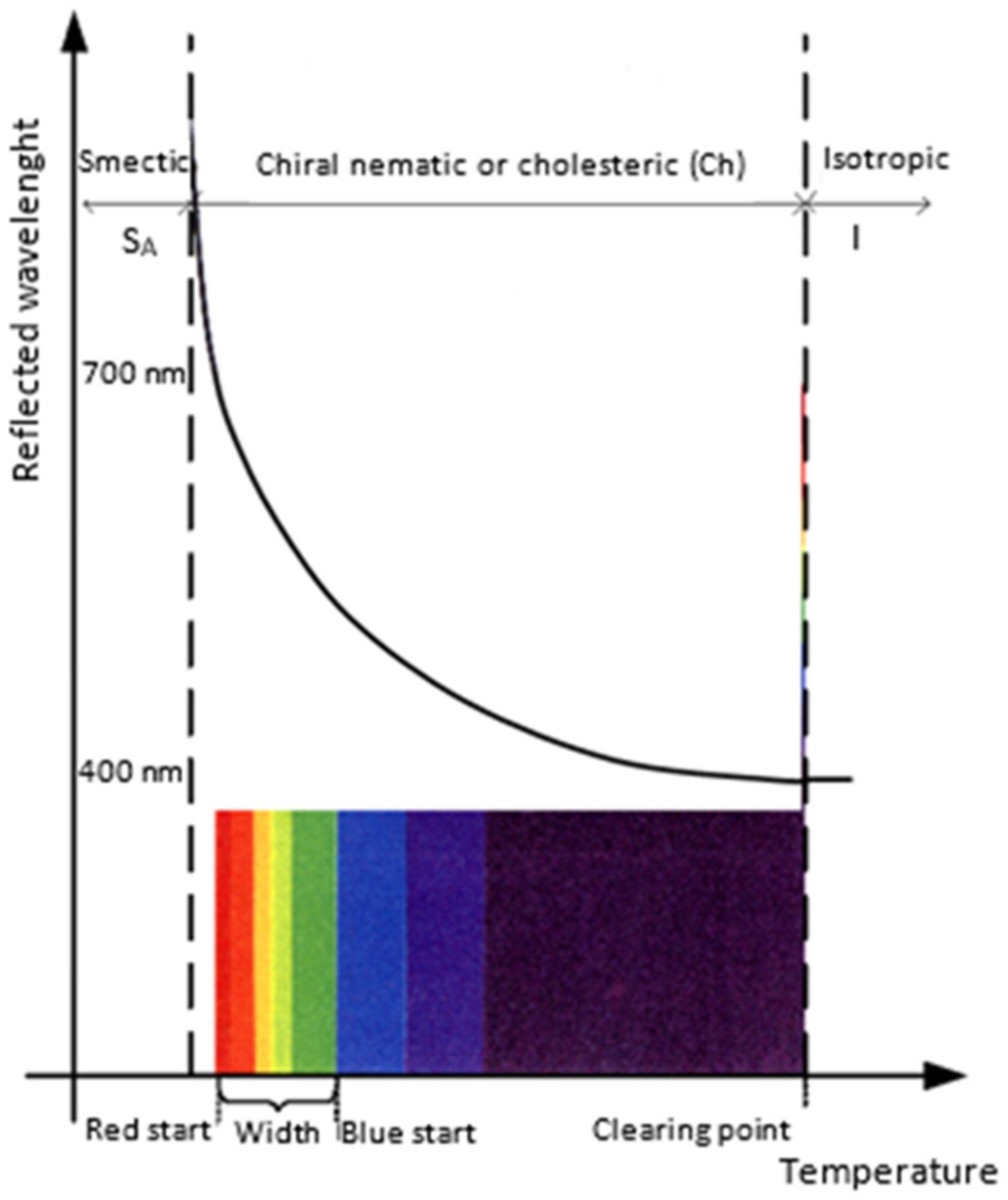
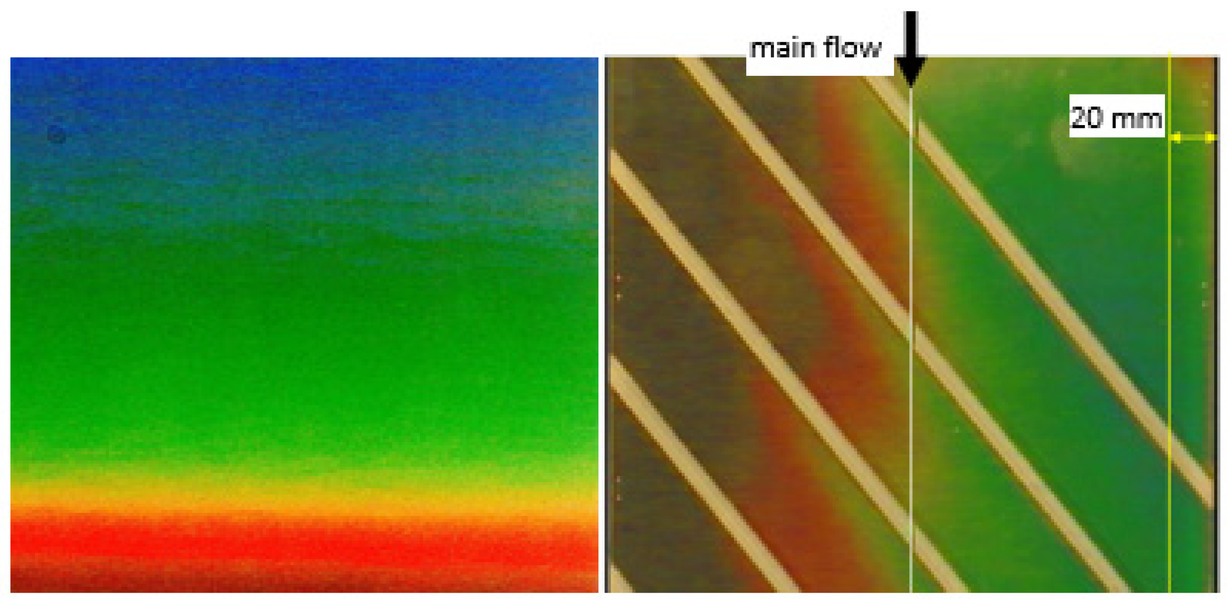
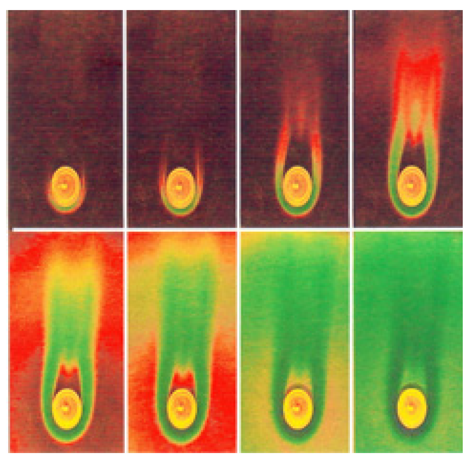
2.1. Liquid Crystals as a Temperature Meter

The history of research on liquid crystals begins over 130 years ago. In 1888, an Austrian botanist F. Reinitzer [39] accidentally discovered the “anomalous” behavior of cholesteryl benzoate during heating. This compound melted at 145.5 °C. The resulting liquid, however, was not clear: it had a very high viscosity and showed color effects. It was not until a temperature of 177.5 °C was reached that the transition to the transparent liquid took place. The German physicist O. Lehmann [38] became interested in this phenomenon, recognizing the state of a turbid liquid as a separate state of matter which he named a liquid crystal. Currently, an alternative term is also used—mesophase (from the Greek mesos—intermediate). Liquid crystals, after several decades of collecting research material, have found application in science and technology, initially in thermography and defectoscopy, and then in the detection of organic compounds, electromagnetic radiation and ultrasound. At present, many different supermolecular structures are known to exist in liquid crystalline states; one of these screw-shaped structures (helicoids) is the so-called cholesteric liquid crystals (ChLC). Cholesteric liquid crystals, similar to other mesophases, are anisotropic and the helicoid structure causes them to exhibit special optical properties, such as selective light reflection or strong twisting of the plane polarization of transmitted light, as is the case with brilliant crystals. The liquid crystal as an indicator of temperature causes the dispersion of white light showing the color of the rainbow, whose reflected wave is proportional to the temperature. When applied to a black surface or suspended in a liquid, it can serve as a color temperature indicator. Normally transparent or slightly milky liquid crystal changes its appearance in the temperature range called “color play interval”, which is the temperature range varying from red, orange, yellow, green, blue, dark navy blue to scarlet (Figure 1). Color play range and event temperature (red start) depend on the composition of the liquid crystal and will vary from −30 to 140 °C and the width of the visible band from 0.5 to 20 °C. Liquid crystals with a measuring bandwidth of 0.5 °C are called narrowband, while the ones with a width greater than 5 °C are called wide band. The selection of the temperature indicator (liquid crystal) will depend on the measurement conditions and the image interpretation technique.

The thermo-optical phenomenon occurring in the TLC can be used in two ways:

• By applying the liquid crystal to the test object as an alloy or solution in a suitable solvent,
• By using the encapsulated forms in the coated (printed) sheets or slurries.

The first method generally requires prior coating of the test object with a layer of black and is time-consuming and expensive (and requires regeneration of the liquid crystal used). Moreover, the TLC layer is not protected against the harmful influence of external factors, which may disturb the measurement process. For these reasons, the first method is used only when the complex shape of an object prevents the use of encapsulated layers. To make such a layer, it is necessary to enclose the TLC in a medium transparent to visible light, isolating the liquid crystal substance from harmful environmental influence and enabling multiple uses. The next step consists of creating a layer of the encapsulated TLC with the desired dimensions, but with low thickness, and low heat capacity, i.e., a short reaction time, and applying other technological layers on the created layer, e.g., black absorbent paint, encapsulating TLC and adhesive materials, etc. [38].

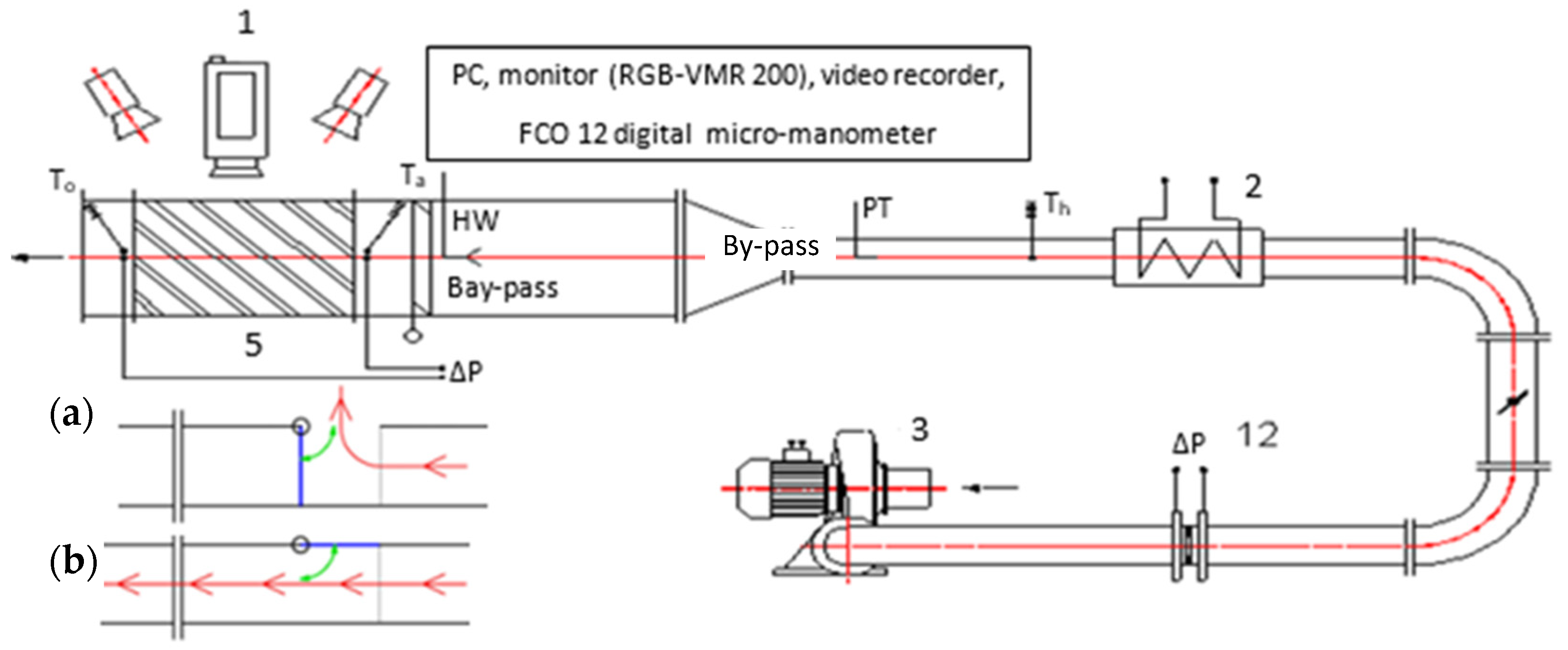
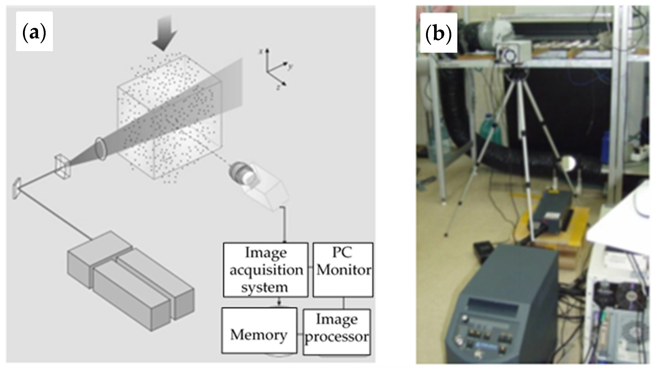
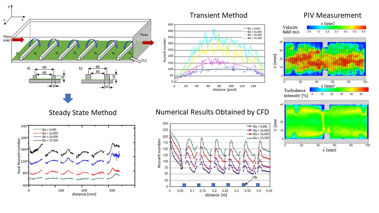
2.2. Experimental Stand

The experimental stand was designed and built at the Gdańsk University of Technology, Faculty of Mechanical Engineering, Poland. Figure 2 shows an open low-speed wind tunnel for physical modeling of a model heat exchanger. The most important components of the wind tunnel are, among others, a fan, an air heater, an initial section that stabilizes the flow, large settling chambers and a TLC test section. The stand is equipped with the MPA 90T fan with a maximum capacity of 1200 nm³/h with automatic and smooth speed control by means of an inverter, which allows obtaining Reynolds numbers Re to a value of about 1.5 × 10⁵ in the test section with hydraulic diameter D_h = 69.11 mm. Inside the control section, the measurement of the amount of air flow and its parameters is carried out using a Pitot tube and a FC012 digital micro-manometer from Furness Controls Limited UK.

This part of the control section is also used to calibrate the hot wire anemometer probe (DISA-thermo anemometer type 55M01). The last part of the wind tunnel is the bypass valve system (Figure 2a,b) enabling the heated air to flow through the measuring sections after reaching the assumed initial temperature T_a. The air tunnel has been equipped with J-type thermocouples for measuring the air temperature in the tunnel and in the measuring section (from the ambient side) to assess, among others, heat losses by convection.

The measurement test section is illuminated from above with a set of tungsten lamps and the color images are recorded with the use of a computer-vision system.

The measuring section or TLC test section is a W = 254 mm wide and H = 40 mm high and L = 550 mm long flat channel made of 8 mm thick plexiglass. The shape and dimensions of the test section are shown in Figure 3. The temperature of the surface (with ribs) to which the heat is applied from the hot air is measured via a liquid crystal foil (R30C5W) attached to the bottom surface of the test section. The color images are captured through the second, upper, transparent surface of the channel. The knowledge of the heat flux density and the local temperature values obtained by liquid crystal thermography makes it possible to calculate the local values of the heat transfer coefficients or Nusselt numbers. Figure 4 shows five different configurations of the ribs in the measuring section.

(1)

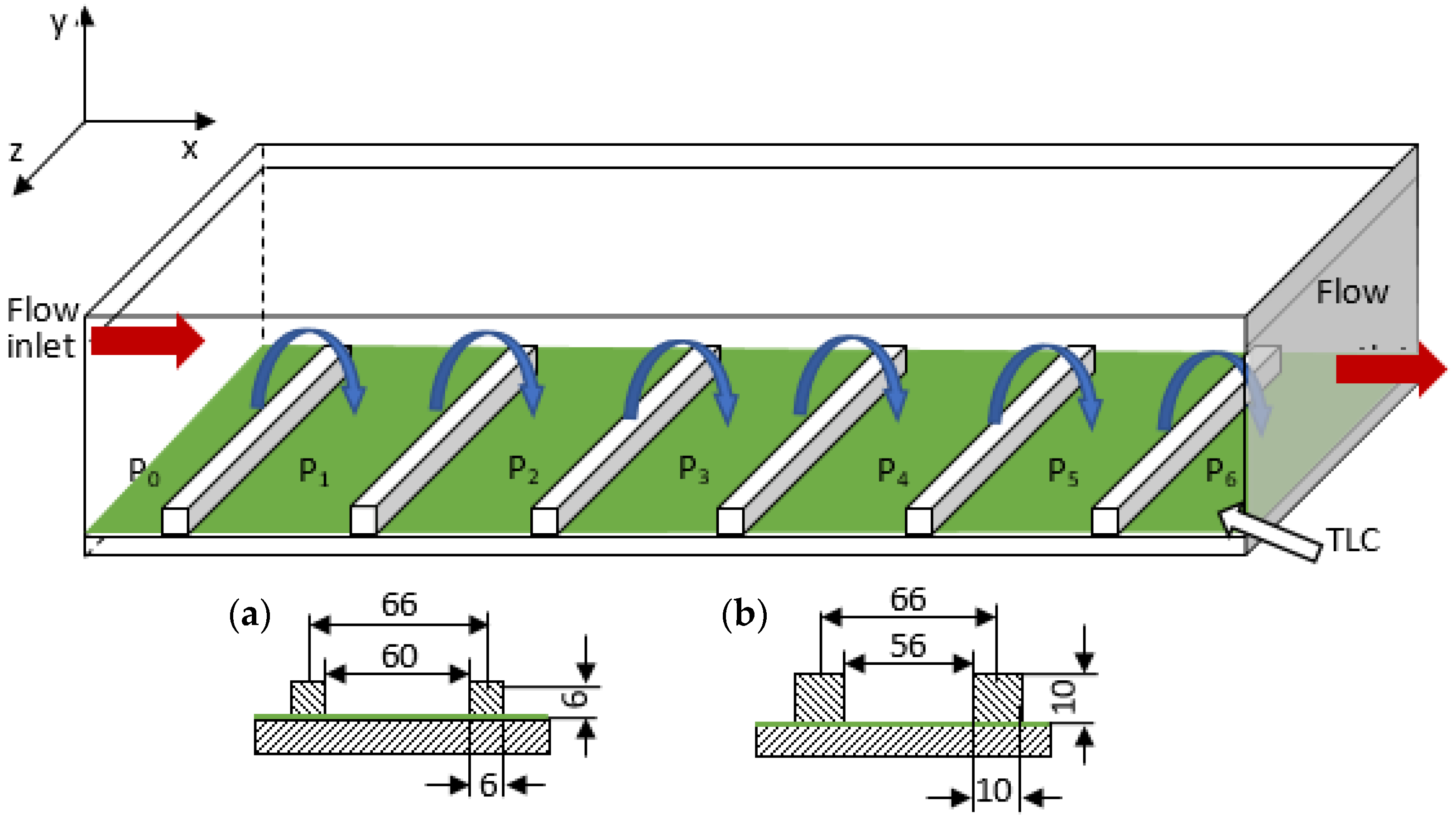
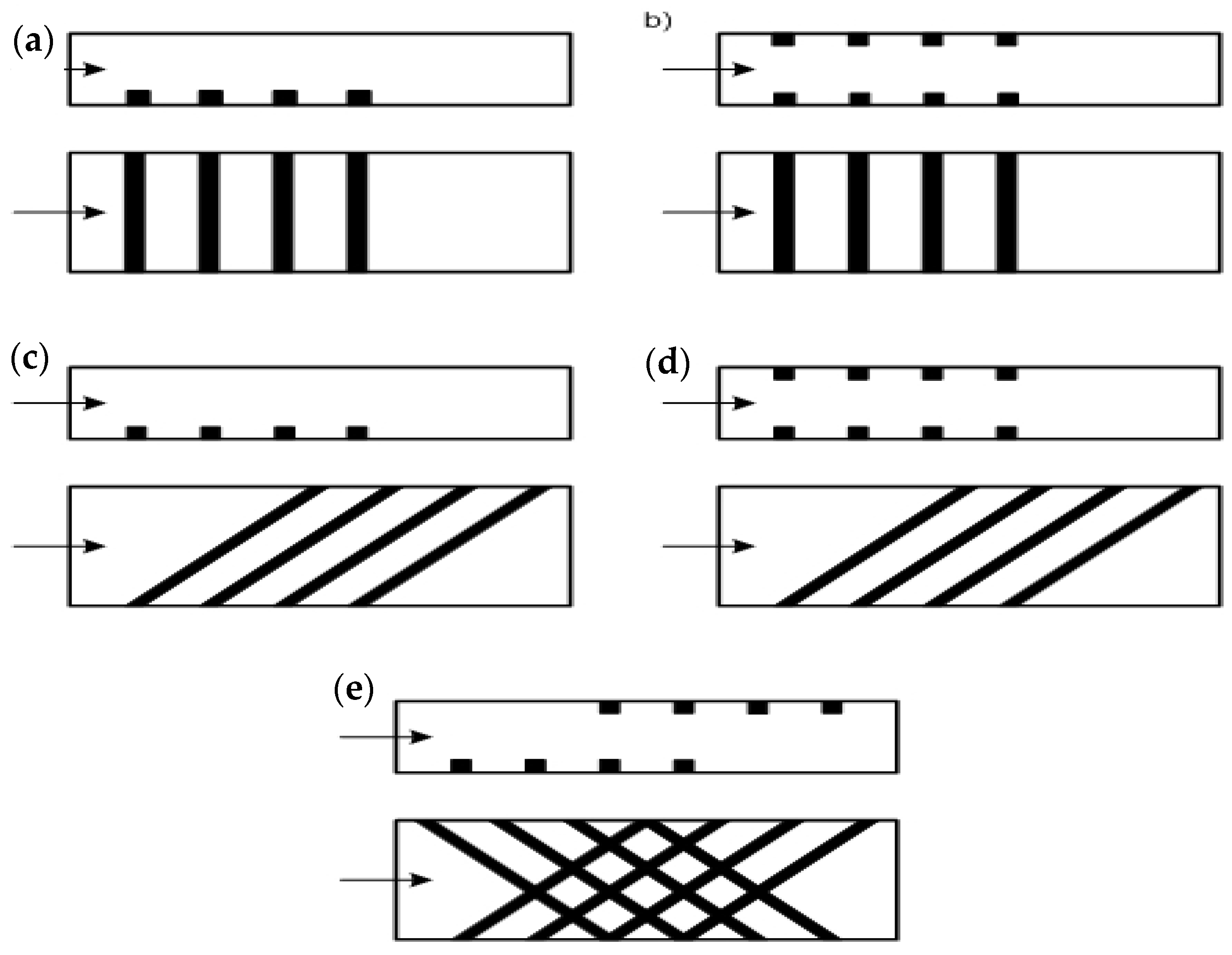
configuration_1 (6 mm straight bottom): only the bottom wall of the duct ribbed with six ribs 6 mm wide and square cross-section; ribs perpendicular to the direction of incoming air; distance between rib centers: 66 mm (60 mm between rib edges), P/e = 11;

(2)

configuration_2 (6 mm straight bottom-up): bottom and top wall of the duct ribbed with six ribs (each wall) 6 mm wide and square; ribs perpendicular to the direction of incoming air; distance between rib centers: 66 mm (60 mm between rib edges) P/e = 11;

(3)

configuration_3 (6 mm 45°): only the bottom wall of the duct ribbed with six ribs 6 mm wide and square; ribs at an angle of 45° to the direction of incoming air; distance between rib centers: 66 mm (60 mm between rib edges) P/e = 11;

(4)

configuration_4 (6 mm 45°–45°): bottom and top wall of the duct ribbed with six ribs (each wall) 6 mm wide and square; ribs at an angle of 45° to the direction of incoming air and parallel to each other; distance between rib centers: 66 mm (60 mm between rib edges) pseudo laminar P/e = 11;

(5)

configuration_5 (6 mm 45°–135°): lower and upper duct wall ribbed with six ribs (each wall) 6 mm wide and square; ribs at an angle of 45° to the direction of incoming air and perpendicular to each other; distance between rib centers: 66 mm (60 mm between rib edges) P/e = 11;

(6)

configuration_6 (10 mm straight bottom): only the bottom wall of the duct ribbed with six ribs 10 mm wide and square in cross-section, ribs arranged perpendicular to the direction of incoming air; distance between rib centers: 66 mm (56 mm between rib edges) P/e = 6.6;

(7)

configuration_7 (10 mm straight bottom-up): bottom and top wall of the duct ribbed with six ribs (each wall) with a width of 10 mm and a square cross-section; ribs perpendicular to the direction of incoming air; distance between rib centers: 66 mm (56 mm between rib edges) P/e = 6.6;

(8)

configuration_8 (10 mm 45°): only the bottom wall of the duct ribbed with six ribs 10 mm wide and square; ribs at an angle of 45° to the direction of incoming air; distance between rib edges: 66 mm (56 mm between rib edges) P/e = 6.6;

(9)

configuration_9 (10 mm 45°–45°): bottom and top wall of the duct ribbed with six ribs (each wall) with a width of 10 mm and a square cross-section; ribs at an angle of 45° to the direction of incoming air and parallel to each other; distance between rib edges: 66 mm (56 mm between rib edges) P/e = 6.6;

(10)

configuration_10 (10 mm 45°–135°): bottom and top wall of the duct ribbed with six ribs (each wall) with a width of 10 mm and a square cross-section; ribs at an angle of 45° to the direction of incoming air and perpendicular to each other; distance between rib edges: 66 mm (56 mm between rib edges) P/e = 6.6.

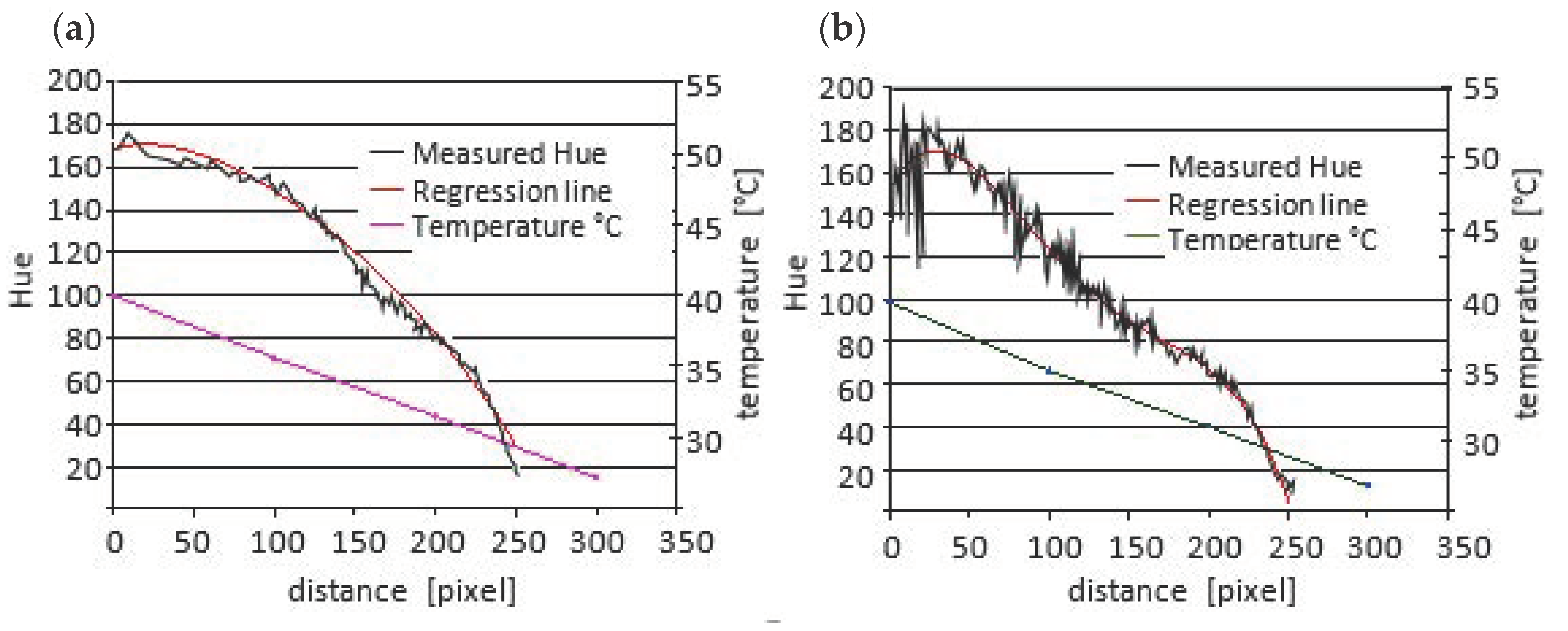
2.3. Calibration of Liquid Crystal-Coated Sheets

The surface temperature was assessed on the basis of hue measurements, which were then converted to Kelvin or Celsius temperature using the liquid crystal layer gauge curve. The hue value and also the temperature were read with an accuracy of one pixel along the measuring length. Experimental procedures of temperature measurement cover full field flow patterns in classic heat exchanger elements (flat plate with ribbed elements) describing the local heat transfer coefficient and Nusselt number on the surfaces. The visualization of such results is presented in Figure 5.

Before starting the planned measurements of the temperature fields and their visualization, a complete assessment of the measuring instruments (color or black and white camera), lighting and quality of liquid crystals should be made. The dependence of the reflected light on the liquid crystal and the temperature should be determined in laboratory conditions, i.e., in the conditions of the measuring section. The calibration plate to which the liquid crystal foil was attached was made of brass with an appropriately regulated linear temperature. To calibrate the liquid crystal foil, i.e., to determine the dependence of the hue (the hue is one of the HIS color scales) on the temperature, halogen and tungsten lighting were used. However, the method of calibrating the liquid crystal foil can be derived, among others, from the papers [6,20,25]. As was mentioned before, the calibration was performed with the use of halogen and tungsten lighting (Figure 6). The obtained values showed that the halogen lighting has much smaller oscillation of the hue value, and therefore, it was selected for further measurement procedures.

2.4. Steady State Analysis by the Constant Heat Flux Method

Early studies of heat transfer performance of ribbed channels employ an electrically heated model and the TLC was used to monitor the surface temperature. HR5534R23.4L12F plate heater from MINCO Products Inc. (Minneapolis, MN, USA) was used to generate a steady heat flux. The plate heater with a thickness of 1 mm brought the heat to a thin, 0.5 mm thick, acid resistant steel to which a liquid crystal foil was attached. The heat flux supplied to the liquid crystal layer and then transferred to the cold airflow over the ribbed measuring section is the result of four heat fluxes, and in particular for the heat flux from the plate heater, from halogen lamps. Heat losses to the environment from the lower surface of the measuring section and radiation heat transfer rate to the surroundings can be calculated as follows:

Q_conv = Q_el + Q_hal − Q_los − Q_rad

(1)

where

• Q_el—is the measured input power to the plate heater,
• Q_hal— is the heat supplied by halogen lighting,
• Q_los— is the heat losses to the environment by free convection,
• Q_rad— is the radiative heat transfer rate to the surroundings.

Finally, after taking into account all losses and gains of the heat, the heat transfer coefficient h was calculated using the following equation:

h = Q_conv/A(T_w − T_a) = q_conv/(T_w − T_a)

(2)

where T_w is the ribbed surface temperature given by TLC, T_a is flow air temperature, A is the area of ribbed section and q_conv is the convection heat flux.

The sum of Q_hal, Q_los and Q_rad was typically equal to 10–15% of Q_el for P/e = 6.66 and 5 to 10% for P/e = 11, depending on the test conditions and increased input power from the heater.

This technique had been used by many researchers for the evaluation of heat transfer coefficients by recorded isoline (selected hue interval from the color map) using color image processing techniques [6,7,13,21].

2.5. Transient Method Analysis

The transient method requires the measurement of the elapsed time to increase the surface temperature of the TLC-coated test section from a known predetermined value of initial temperature (T_i). The main advantages of this method are that no continuous heating of the tested model is required and measurement of the size when examining complex shapes is easier. Jones et al. [29] appears to be the first to use this technique to measure temperature. The data collected during such an experiment consist of a series of photos or a film in which the successive phases of the appearance of a surface covered with liquid crystal are recorded. The isolines that appear on the surface are related to the temperatures in the calibration process, so they are actually isotherms. Jones and Hippensteele [40] compared this method with the steady state method. A similar experiment was also carried out by Baughn et al. [11] in an electrically heated ribbed channel. Both Jones and Baughn noticed differences in the obtained results yielding from the determination of the temperature boundary condition for both cases. Interpretations of the differences in the obtained results can be found in the work of Jones et al. [29]. In the 1990s, intensive research using the transient method was also conducted by Leiner et al. [30]. The heat transfer to the object is recorded by a video camera recording the color changes (temperatures) of the liquid crystal layer over time—the time history of the color changes of the liquid crystal layer as shown in (Figure 7).

If the object is made of a material with low thermal diffusivity and sufficient thickness, the occurring phenomena of heat exchange can be considered one-dimensional. The relationship between the wall surface temperature and the heat transfer coefficient is expressed by the formula given by Jones et al. [29]:

$$\frac{T-T_i}{T_a-T_i}=1-e^{{\beta }^2}erfc\left(\beta \right)$$

(3)

where:

$$\beta =h{\left(\frac{\tau }{\rho ck}\right)}^{0.5}$$

(4)

In the above relation, ρ, c and k denote the density, specific heat and thermal conductivity of the model material (plexiglass), T_i is the initial temperature, T_a is air temperature and τ is the interval time from the beginning of the plate heating. Leiner et al. [30] presented another formulation of this relationship, which is expressed in the Formula (5):

$$h=\frac{-x\rho c}{2\tau }\ln \left[\frac{T_a-T}{T_a-T_i}\right]$$

(5)

where x is a plexiglass plate thickness with liquid crystal foils and the local surface temperature T detected after interval time τ.

The distributions of local heat transfer coefficients h and Nusselt numbers Nu were determined for one section in four configurations for the full research range, i.e., for each measurement pixel in the p4 section (behind the fourth measurement rib).

The analysis of the mid-section p4 aims to establish the flow behavior depending on the configuration of flow turbulators used. This section best reflects the nature of the air stream that prevails in real heat exchangers in the areas of the most efficient operation of the exchanger—it is, therefore, a representative of the comparisons of various methods.

2.6. Particle Image Velocimetry Anemometry

PIV technique is another well-established experimental method in fluid mechanics that allows quantitative measurement of two- (2D) or even three-dimensional (3D) flow structure [9]. More recently, this technique has been applied to study heat and fluid flow in complex geometries with highly non-uniform boundary conditions. Currently, 2D PIV measurements were performed for pure air seeded with small droplets (few micrometers in diameter) of synthetic oil DEHS (Di-Ethyl-Heksyl-Sebacat). The oil drops volumetric concentration was very low, so they did not affect the flow structure. PIV used in presented experiment is shown in Figure 8. The tested flow with the addition of marker particles is illuminated by a narrow plane of light, the so-called light knife. A green laser beam was used as the light source from which the light beam is directed to the tested flow and formed into a light knife by means of a system of mirrors and a cylindrical lens.

The displacement of the moving marker particles is determined by correlating the fragments of two images recorded at a known time interval. Fast Fourier transform (FFT) is used to calculate the correlation function between the fragments of the analyzed images. By analyzing the change in particle position for the previously defined image regions, the average displacement for this selected fragment is determined, i.e., the average flow velocity in this fragment. The lower limit is confined by the minimum number of particles in the recorded image fragment, necessary for the determination of the correlation function.

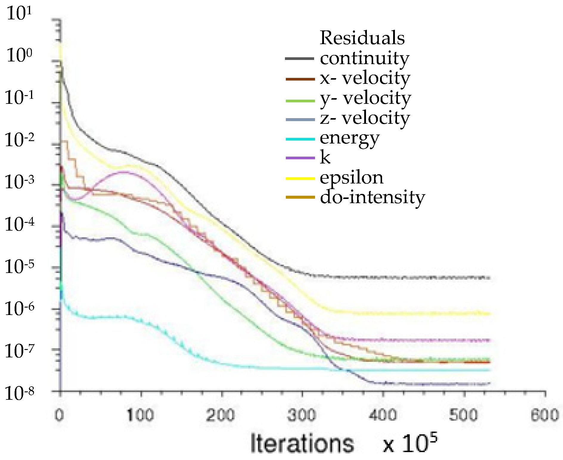
2.7. Computational Fluids Dynamics—CFD

The dynamic development of technology and the increase in computing power have resulted in the successive displacement of analytical methods in favor of numerical ones. Modern flow simulations are usually carried out with the use of the Computational Fluids Dynamics method (CFD). One of the environments based on CFD is the ANSYS Fluent code package which allows modeling of complex phenomena related to flows, such as combustion, turbulence, multiphase flows, chemical reactions, heat conduction, radiation, etc. The turbulence models available in ANSYS Fluent include Detached Eddy Simulation (DES), Large Eddy Simulation (LES) and Reynolds Averaged Navier-Stokes Equations (RANS). RANS distinguishes between single-equation (Spalart-Almaras model) and more-equation models, such as k-ε standard, RNG k-ε, k-ω standard, SST k-ω and the Reynolds stress model. More information on turbulence models and calculation methods can be obtained in the ANSYS Fluent package [37] and A. Stasiek’s doctoral dissertation [28]. Numerical modeling of turbulent flows is also presented in the works [5,13,21,28]. The k-ε model proposed in 1974 by Launder and Spalding [41] and CFD FLUENT software by ANSYS Inc. (Southpointe 2600 Ansys Drive Canonsburg, PA 15317, USA) was selected to verify the thermographic measurements of the model heat exchanger (flat duct with rib-shaped mechanical turbulators). Finally, in these works, it was shown that k-ε not only models the issues discussed in presented article thoroughly, but it is also time-saving, fast and accurate in calculations. In order to carry out numerical calculations, it was necessary to initially assume the level of turbulence intensity, which was obtained both from the PIV measurements and hot-wire (see Figure 2 and Equation (11)). Calculations for each case were carried out until the solution values stabilized in a range of variability from 10⁻⁵ to 10⁻⁹ (see Figure 9). For example, the grid representing the measurement section for Re = 9000 was composed of 576,000 cubic elements. Each simulation was performed with the same calculation parameters and identical boundary conditions. The only differences are in the value of the inlet velocity, which was determined earlier.

3. Results

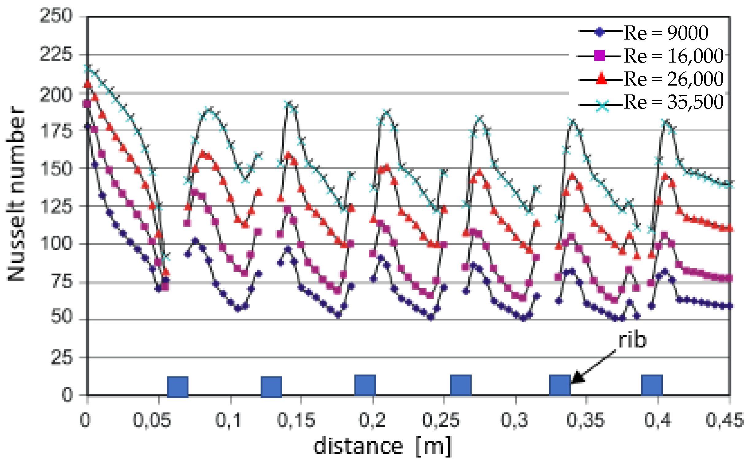
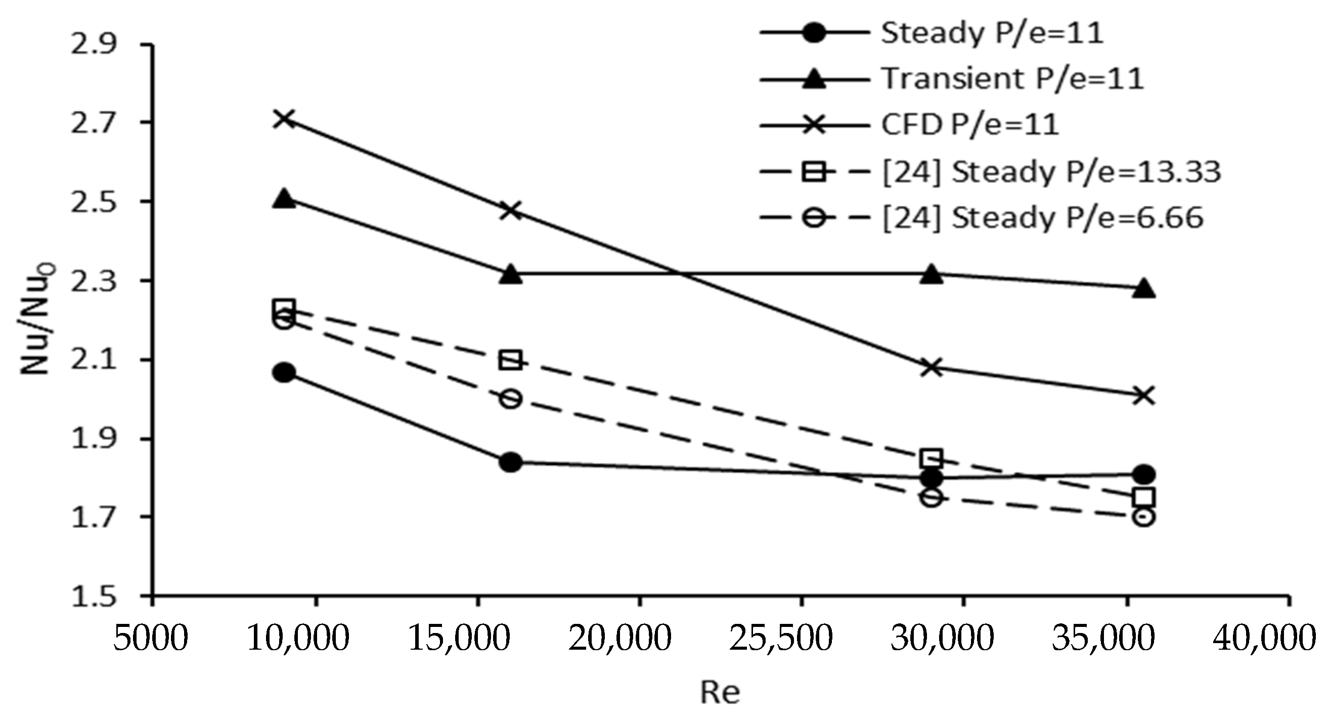
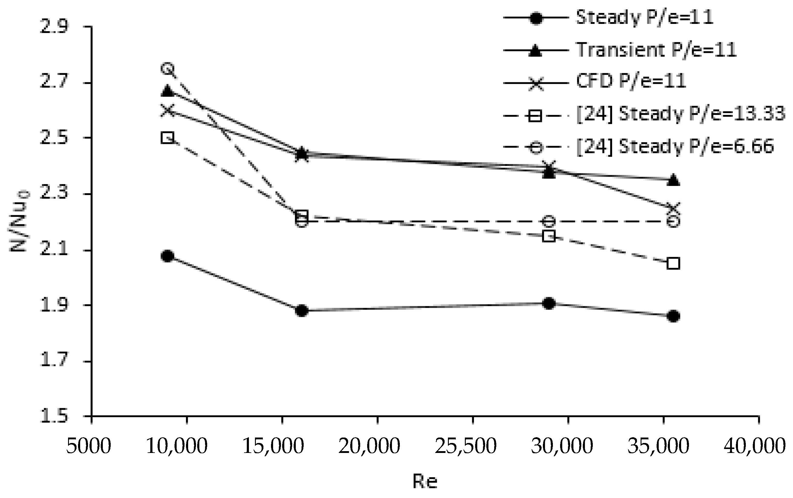
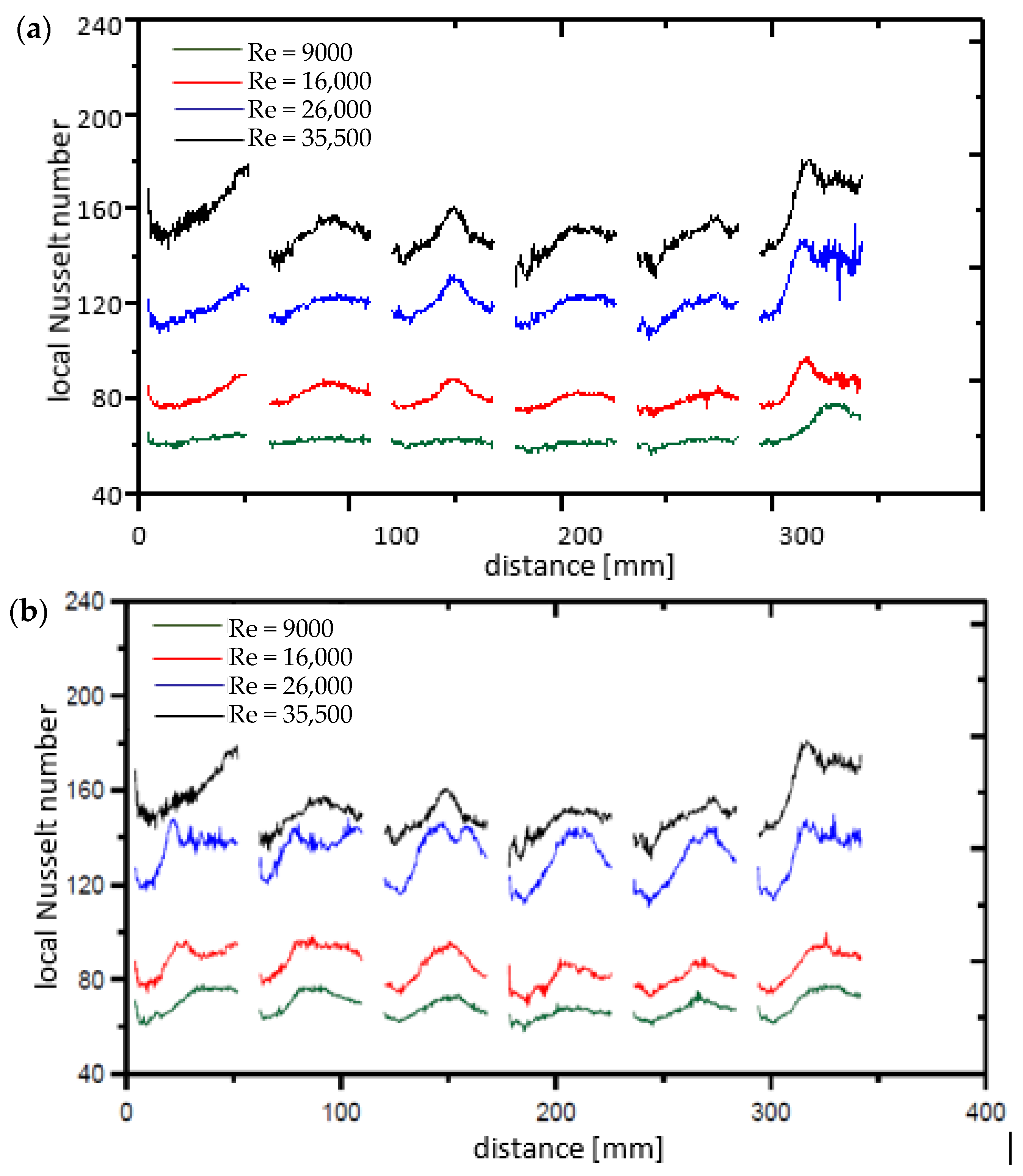
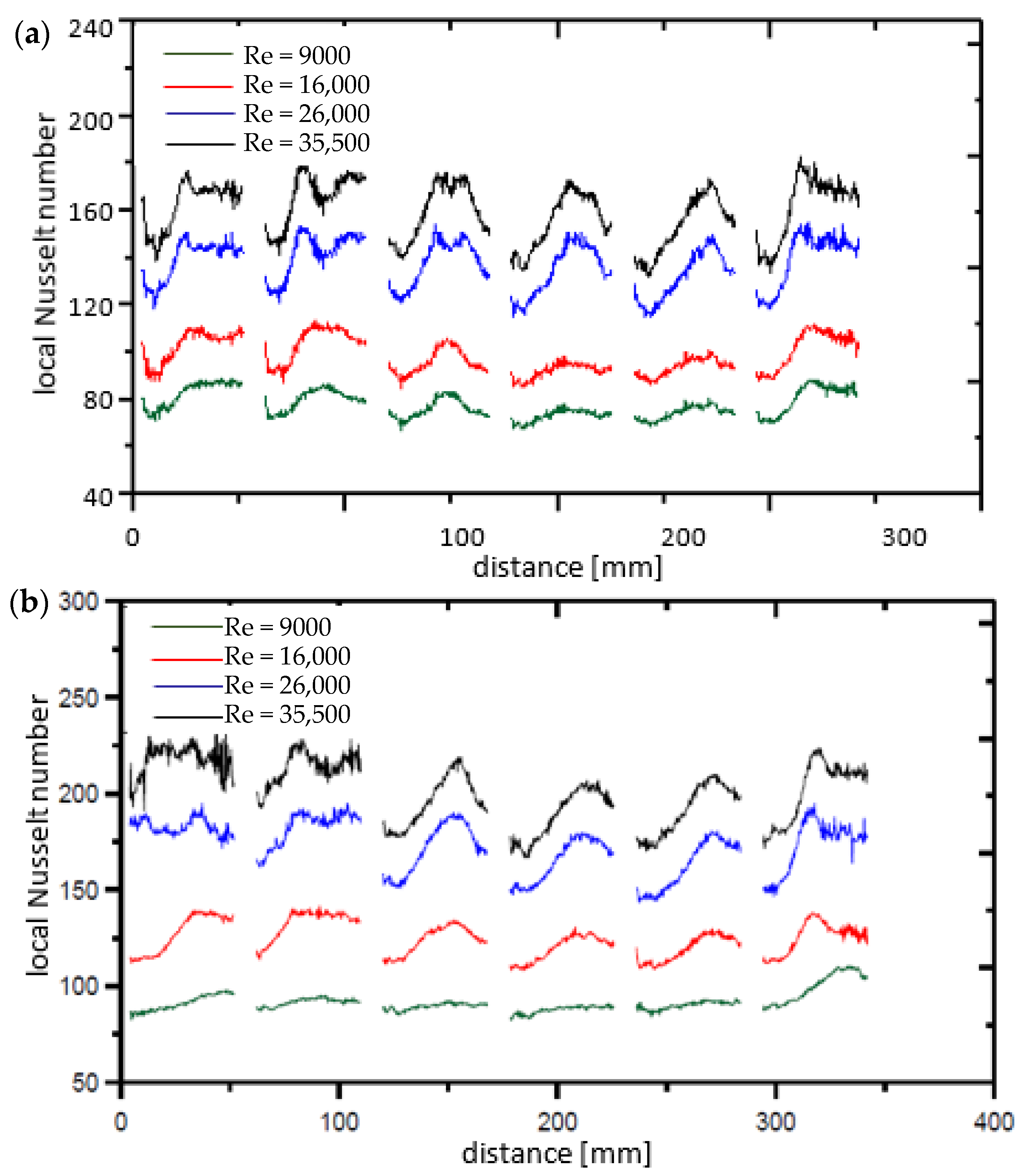
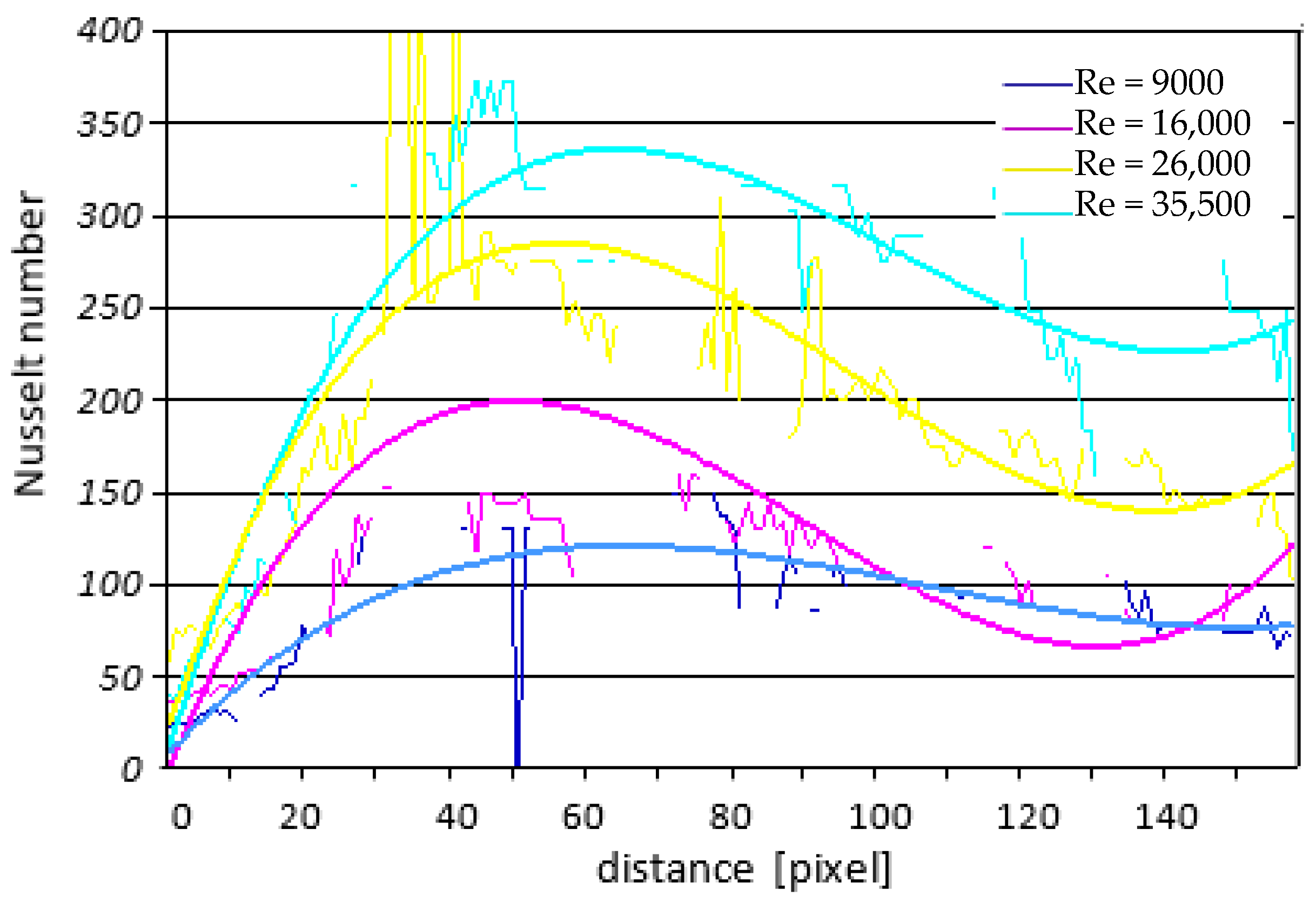
3.1. Experimental Results by the Steady States Method

Experimental data were transformed in dimensionless form, introducing the Nusselt number Nu and the Reynolds number Re as follows:

$$Nu=h{D}_h/k$$

(6)

$$Re=\stackrel{\leftharpoonup }{u}{D}_h/\upsilon$$

(7)

where h is the heat transfer coefficient, D_h the channel hydraulic diameter, ū mean velocity, k thermal conductivity and υ kinematic viscosity evaluated at the air temperature.

Figure 10 and Figure 11 present selected results (configuration_6 and _7) of the distribution values of local Nusselt numbers in the middle zone and near the side wall. As mentioned earlier, the research was carried out for four values of Reynolds number, 9000, 16,000, 26,000 and 35,500, and a 10 mm high rib. The analysis of the presented graphs shows that surface with straight ribs yields the best effects (the highest mean values of the heat transfer coefficient). The values of the latter are also higher for the ribs that are lower. Obviously, the presence of turbulators contributes to a further improvement of the heat transfer coefficient or Nusselt number. Presented thermographic measurements were made with the use of a liquid crystal foil with ribs attached to an electrically heated metal plate generating a constant heat flux.

For comparison purposes, Figure 11 and Figure 12 show the distribution of local Nusselt numbers for configuration_6 and _7 in the central and at the wall zone of the test section. In the case of ribbing of one wall of the test section, the differences in the Nusselt number are small. The ribbing of two walls increases the Nusselt numbers by about 19% at the tunnel wall zone compared to the measurements in the central zone, which is the result of diagonally arrange ribs which increased turbulence and partial flow of air towards the side walls of the measuring (test) section.

Table 1. Values of averaged Nusselt numbers (Nu_av) for six measuring sections (p1, p2, p3, p4, p5, p6) and averaged for the whole plate.

Nuav
	Re	p1	p2	p3	p4	p5	p6	Nuav
Conf_1	9000	66.53	65.40	62.34	58.11	57.41	65.18	62.49
	16,000	102.58	100.27	97.51	95.05	95.11	108.28	99.80
	26,000	140.04	140.88	135.55	127.91	126.17	142.88	135.57
	35,500	172.41	175.69	171.68	162.48	162.39	184.31	171.49
Conf_2	9000	85.11	84.36	87.09	84.60	83.73	94.44	86.55
	16,000	130.81	131.15	126.37	122.65	121.01	135.24	127.87
	26,000	172.57	172.98	172.25	168.10	167.63	185.68	173.20
	35,500	212.03	213.63	211.62	207.78	204.67	222.39	212.02
Conf_3	9000	60.15	60.88	60.88	60.21	57.59	64.96	60.78
	16,000	88.26	87.31	86.14	84.05	83.73	96.23	87.62
	26,000	118.10	122.66	121.74	122.61	117.56	113.54	119.37
	35,500	153.72	160.76	156.67	157.25	154.14	155.94	156.41
Conf_4	9000	59.00	60.30	60.17	59.82	59.84	59.47	59.77
	16,000	85.36	86.11	86.22	86.64	87.33	84.85	86.09
	26,000	126.10	132.26	129.21	129.93	127.14	129.13	128.96
	35,500	155.48	163.43	161.59	161.53	154.86	163.78	160.11
Conf_5	9000	62.18	64.90	61.76	60.80	58.68	61.74	61.68
	16,000	86.60	88.70	84.89	83.00	80.90	87.21	85.22
	26,000	128.67	134.23	126.45	125.87	125.87	133.42	129.08
	35,500	152.97	155.70	154.04	155.49	152.15	155.48	154.30
Conf_6	9000	63.07	62.88	62.05	60.93	61.88	69.69	63.42
	16,000	81.76	83.35	81.64	79.72	79.22	86.66	82.06
	26,000	117.90	119.95	121.04	119.07	117.37	134.27	121.60
	35,500	159.66	149.55	148.39	145.72	147.21	164.68	152.54
Conf_7	9000	103.57	100.07	95.16	91.49	93.18	100.96	97.40
	16,000	128.73	129.84	119.80	115.13	117.27	127.39	123.03
	26,000	174.27	177.22	172.20	168.09	165.01	174.92	171.95
	35,500	203.60	207.21	199.56	194.44	191.83	202.54	199.87

shows the local values of the Nusselt number for various geometries and measurement section from p1 to p6, as well as the average values for the whole plate for various Reynolds numbers.

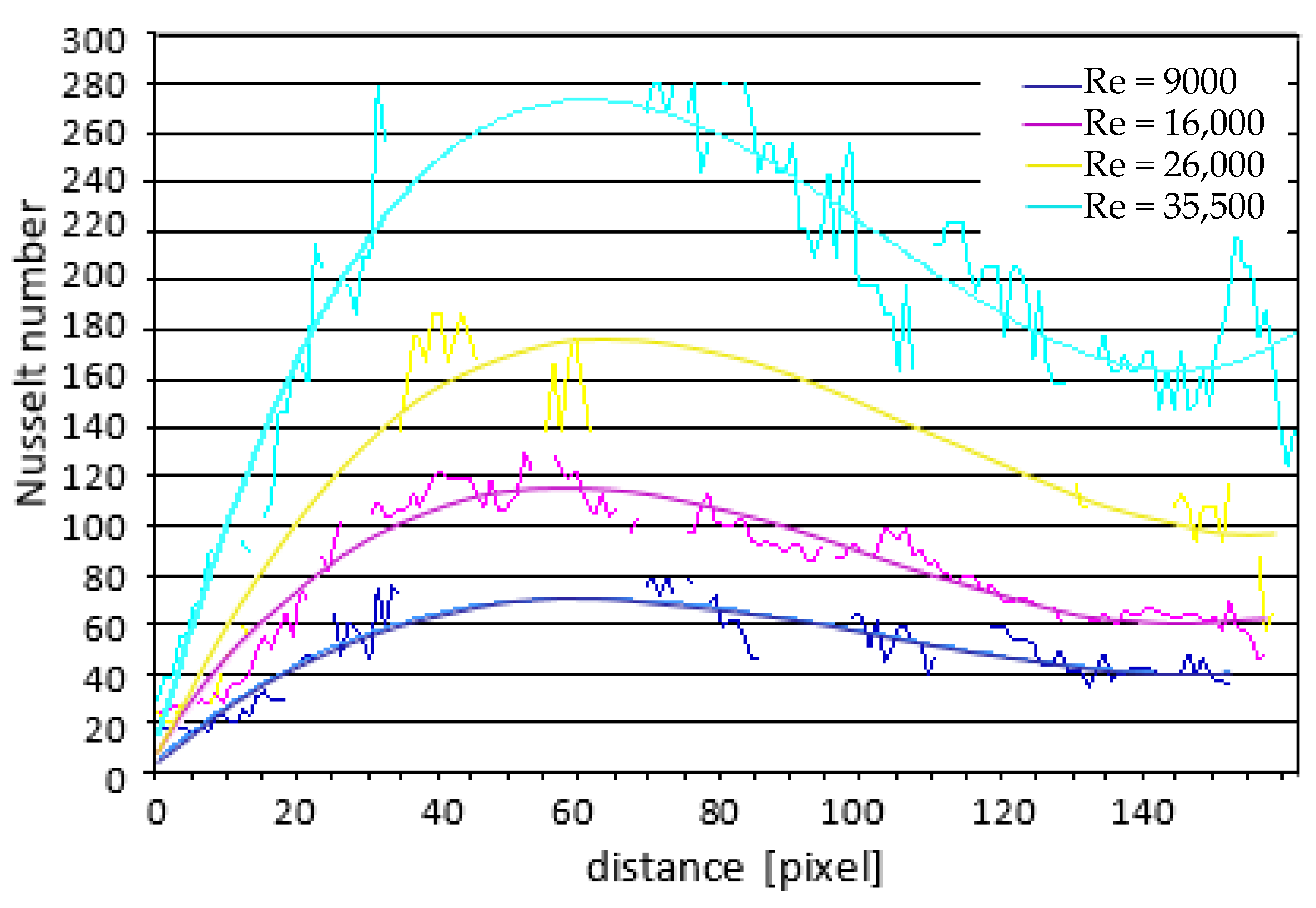
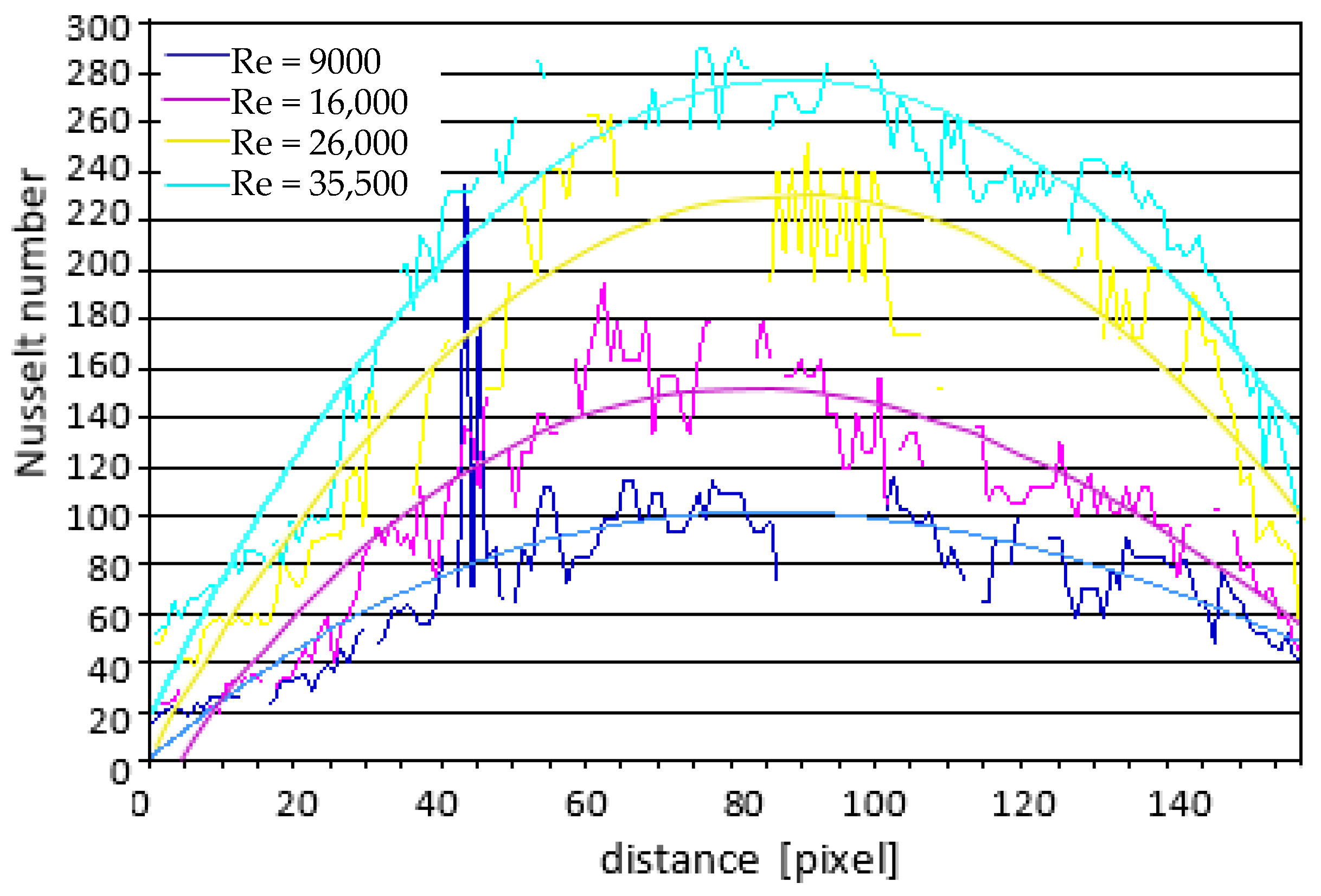
3.2. Results Obtained in the Transient Method

Results of the local Nusselt number for different configuration of the ribs are presented in Figure 12, Figure 13, Figure 14 and Figure 15. Color images representing the temperature field were recorded with a frequency of 50 1/s. The measurement results in the form of Nusselt numbers were then approximated by the third-degree function and for the calculations the temperature T = 303.5 ± 0.1 K was assumed, corresponding to a hue value in the range of 45–55.

When analyzing the distributions of Nusselt numbers obtained from the measurements by the thermographic method (Figure 10, Figure 11, Figure 12, Figure 13, Figure 14 and Figure 15), it is not difficult to notice that the use of ribs as flow turbulators causes, among others:

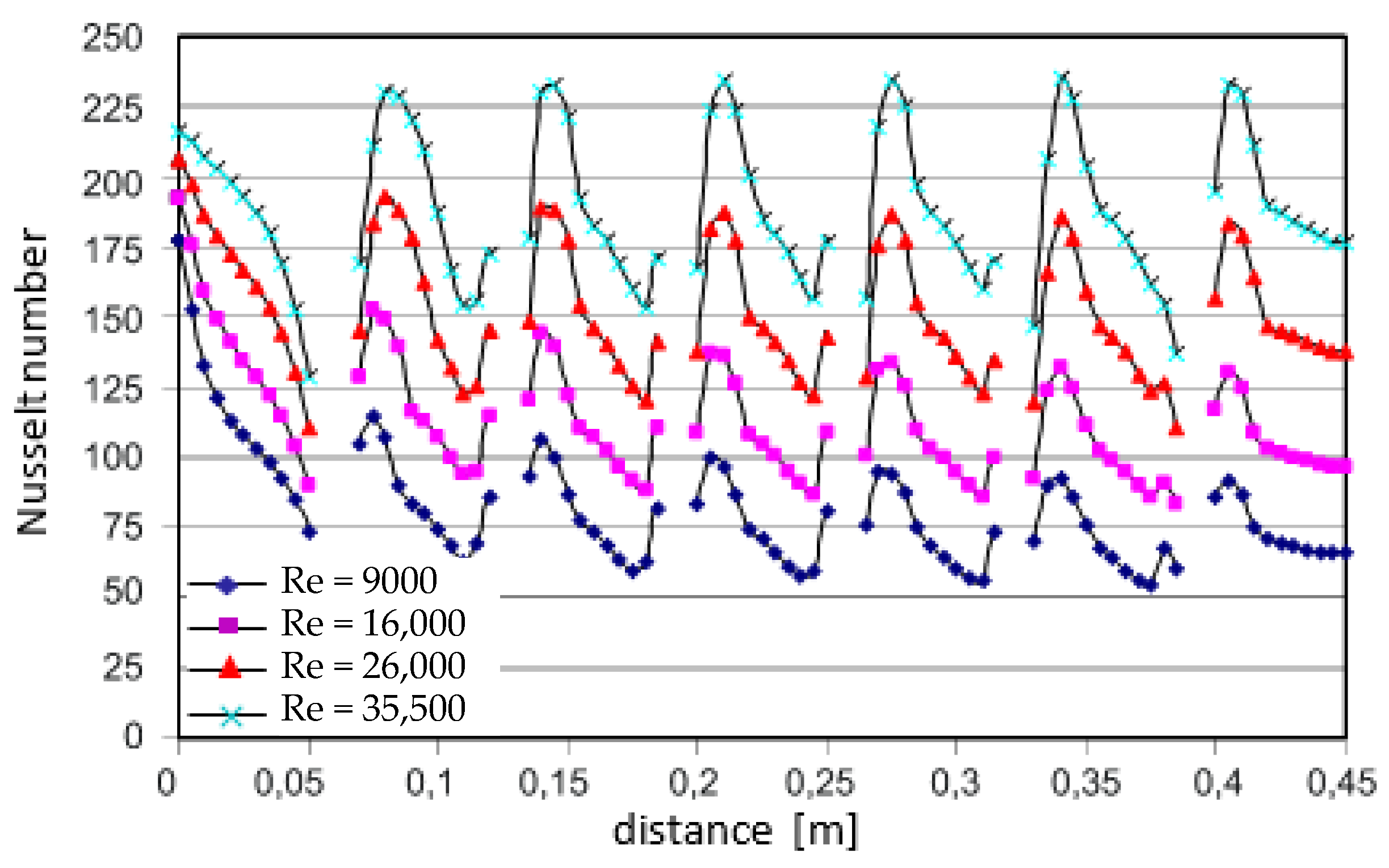
• Multiple increases of heat exchange and flow stabilization,
• Much greater influence on the increase of heat transfer at lower Reynolds numbers—this is confirmed by PIV measurements showing the absence of vortices and no blows or projected jets of air streams on the surfaces between the ribs,
• The influence of the ribs on the stabilization of heat transfer along the ribbed plate was also observed—higher heat transfer coefficients were obtained for the first section of the tested flat surface (entrance effect),
• For larger Reynolds numbers, the influence of the ribs is much smaller, which can be explained by the movement of the air stream above the turbulators—it looks like a pseudo laminar flow.

3.3. Data Reduction and Uncertainty Analysis

Experimental uncertainties were computed by applying the estimation method proposed by Moffat [42]. The uncertainty of a quantity R, which can be assumed to be a function of several variables R = R (x₁, x₂, …, x_n) can be calculated with a high accuracy using a root-sum-square (RSS) combination:

$${\epsilon }_R={\left\{{\displaystyle \sum }_{i=1}^n{\left[\left(\partial R/\partial x_i\right){\epsilon }_i\right]}^2\right\}}^{1/2}$$

(8)

where ε_i is the uncertainty in the ith variable. On the basis of Equations (3) and (6), the experimental uncertainty in heat transfer coefficient h can be calculated as:

$$\partial h/h=1/h{\left\{{\displaystyle \sum }_{i=1}^n{\left[\left(\partial R/\partial x_i\right){\epsilon }_i\right]}^2\right\}}^{1/2}$$

(9)

The variation in the parameters of T_a, T_i, T, x, ρ, c and τ are $\partial$T_a, $\partial$T_i, $\partial$t, $\partial$x, $\partial$c and $\partial$t, respectively, provides the uncertainty in heat transfer coefficient as follows:

$$\frac{\partial h}{h}=1/h\sqrt{\left[{\left(\frac{\partial h_l}{\partial T_a}\mathsf{\Delta }{T}_a\right)}^2+{\left(\frac{\partial h_l}{\partial T_i}\mathsf{\Delta }{T}_i\right)}^2+{\left(\frac{\partial h_l}{\partial T}\mathsf{\Delta }T\right)}^2+{\left(\frac{\partial h_l}{\partial x}\mathsf{\Delta }x\right)}^2+{\left(\frac{\partial h_l}{\partial \rho }\mathsf{\Delta }\rho \right)}^2+{\left(\frac{\partial h_l}{\partial c}\mathsf{\Delta }c\right)}^2+{\left(\frac{\partial h_l}{\partial \tau }\mathsf{\Delta }\tau \right)}^2\right]}$$

(10)

When calculating the maximum error values of the heat transfer coefficient (h) or the Nusselt number (Nu), there occur errors in determining the following parameters: the air temperature ΔT_a = ±0.1 K, the initial temperature of the plate ΔT_i = ±0.05 K, the local surface temperature detected by TLC after interval time τ ΔT = ±0.1 K, plexiglass plate thickness Δx = ±0.1 mm, density of plexiglass with TLC foil Δρ = ±0.05 g/cm³, specific heat Δc = ±0.05 J/g·deg and interval time step Δτ = ±3 s. The Reynolds number had a calculated uncertainty of ±5%, mainly due to an inaccurate determination of the amount of air flowing and its physical properties.

The uncertainty (at the 95% confidence level) in local h_l or Nu_l values was estimated to be ±2.3% for higher Re and ±7.04% for lower Re. The use of plexiglass plates for transient thermographic measurements allows assuming one-dimensional heat conduction and neglecting its lateral flow. Lateral heat flow is about 4% of the main heat flux for Re = 10⁴ [24,25].

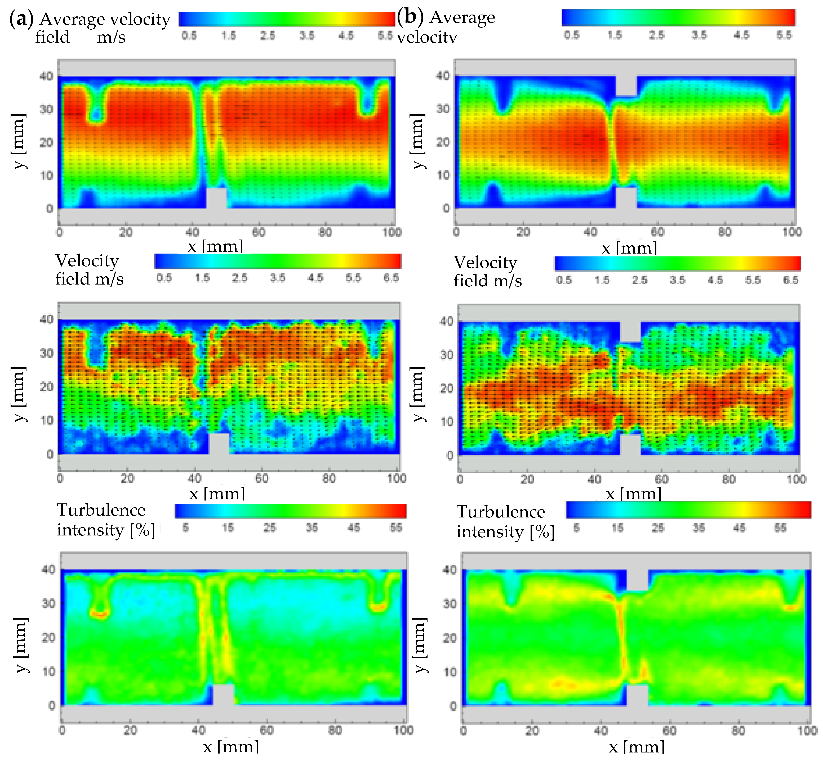
3.4. PIV Measurement Results

The selected results of the PIV measurements are presented in Figure 16. For each experiment, the following is shown:

• Averaged velocity field: vectors and a colored contour of the velocity value,
• Selected instantaneous speed field: vectors and a colored contour of the speed value,
• Turbulence intensity field determined according to the relationship shown in Equation (11).

$$I=\frac{{\left(\frac{1}{n}{\displaystyle \sum _{i=1}^n{\left(u_i-\overline{u}\right)}^2}\right)}^{\frac{1}{2}}}{\overline{u}}\cdot 100\%,$$

(11)

where u_i and $\overline{u}$ are the instantaneous and mean velocity fields, respectively, and n is the number of measurements (instantaneous velocity fields) used to calculate the turbulence intensity and mean velocity field.

Turbulent intensity given by PIV measurement provides useful information for numerical calculations of heat transfer by CFD simulation presented in Section 3.5.

3.5. Numerical Results Obtained by CFD FLUENT

Figure 17, Figure 18, Figure 19, Figure 20 and Figure 21 show the results of numerical calculations of the local Nusselt number for different configurations of rib settings P/e = 11 and different Reynolds numbers, and their average values are presented in

Table 2. Comparison of the Nusselt number determined by three methods: steady state, transient method and CFD for P/e = 11 (section p4).

Re	Nu0	Conf._1			Conf._2			Conf._3			Conf._4			Conf._5
		Nu/Nu0			Nu/Nu0			Nu/Nu0			Nu/Nu0			Nu/Nu0
		St	Tr	CFD	St	Tr	CFD	St	Tr	CFD	St	Tr	CFD	St	Tr	CFD
9000	29	2.01	1.63	2.10	2.91	2.88	2.75	2.07	2.51	2.71	2.08	2.67	2.60	2.19	2.87	2.65
16,000	46	2.06	1.78	2.02	2.67	2.89	2.39	1.84	2.32	2.48	1.88	2.45	2.44	1.88	2.21	2.04
26,000	68	1.89	1.64	1.82	2.47	2.62	2.16	1.80	2.32	2.08	1.91	2.38	2.40	1.85	2.01	2.01
35,500	87	1.87	1.79	1.83	2.39	2.54	2.08	1.81	2.28	2.01	1.86	2.35	2.25	1.79	2.00	1.89

Nu₀—Nusselt number for smooth channel calculated according to the Dittus-Boelter correlation (Nu₀ = 0.023Re^0.8 Pr^0.4), St—steady state, Tr—transient method, CFD—numerical analysis.

.

Numerical calculations performed with the use of the Ansys FLUENT software as a supplement to the thermographic measurements additionally showed the presence of turbulence fields and places of flow stagnation. Places with a reduced amount of heat transfer occur in front of and behind the ribs. Earlier observations regarding the stabilization of the flow after the fourth rib were confirmed. The obtained series of Nusselt number distribution were very similar to those obtained by thermographic studies. However, based on these calculations, it was recorded that bigger changes in the mean values of the heat transfer coefficient h_av, or the Nu occurred for Re = 35,500 as expected. The differences between Re = 9000 and Re = 35,500 were up to 0.35%, which can be seen in Table 2 and Figure 22 and Figure 23. The higher heat transfer parameters were obtained by CFD for an exchanger with oblique ribs placed at an angle of 90° against each other (Configuration_5). The calculated and overestimated values of Nusselt numbers were obtained in comparison to the steady state and transit method for configuration_3, _4 and _5. It requires further analysis and calculation, as these geometries are more complex.

Figure 22 and Figure 23 show the normalized Nusselt number (by Dittus-Boelter correlation) versus the Reynolds number only for configuration _3 and _4 obtained by steady state, transient method and CFD for comparison with the values obtained by Tanda and Abram (steady state method only) [25]. Data from Tanda and Abram for one (1RW) and two (2RW) ribbed wall channels with rib turbulators inclined at 45 degrees were also added to the graph, since the configuration and operating conditions were similar to those considered here. When ribs are applied to the bottom plate only, the larger pitch (P/e = 11) provides a slightly higher heat transfer than the smaller rib pitch (P/e = 6.6), by 7% on average. Adding the ribs to the upper plate increases the turbulence level for both values of P/e and enhanced heat transfer coefficient by up to 25% depending on the Reynolds number and configuration (see Table 1 and Table 2).

As expected, greater scattering of the results obtained with the three methods was observed for the lower Reynolds numbers (including the transition area). Numerical calculations especially gave much higher values of Nusselt numbers for a lower Reynolds number and smaller differences for a higher Reynolds number. The CFD method also gives much higher values of the Nusselt number than the values obtained from liquid crystal measurements using the steady state method. The results obtained with all three methods showed the same trend of the change of the Nusselt number as a function of the Reynolds number. Each method showed the so-called entrance-and-exit effect. All methods also showed large differences in the local values of Nusselt numbers in front of and behind the ribs, indicating the lack of air flow (stagnation effect). The higher heat transfer augmentations occur approximately in the middle between the ribs. In numerical and physical modeling of heat transfer on a ribbed surface, the ribs were treated as flow turbulators not participating in the heat transfer. Comparing the results obtained through these three methods, it seems that the numerical calculations are overstated in relation to the thermochromic measurements and may be the basis for further analysis.

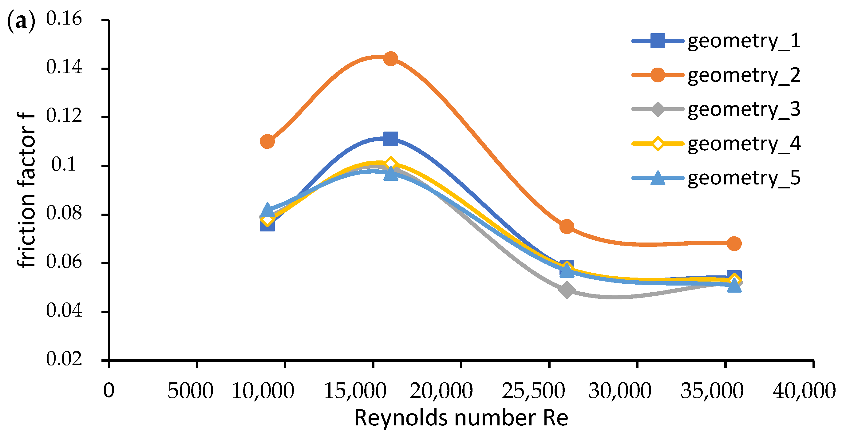
3.6. Friction Factor

In the design of classic and compact heat exchangers, the objective is to obtain the maximum heat transfer coefficients per unit volume; however, enhancing the heat transfer almost always increases the pressure drop, so an optimum design should include an appropriate pressure drop or heat losses. Therefore, heat exchanger designers need to know the heat transfer coefficients h and heat loss ΔP_f or friction factor f to optimize them.

Figure 24 shows the heat loss in form of friction factor f plotted against Reynolds number Re for various configuration P/e = 11 and P/e = 6.6 analyzed in this work. The commonly known Darcy–Weisbach equation and Reynolds analogy [43] were used to make the graphs showing the relation between turbulent momentum and heat transfer, which is described by the following equation:

$$St=\frac{Nu}{Re·Pr}=\frac{f}{8}$$

(12)

or, after transformation:

$$f=\frac{8·h}{c_p·\rho ·u_0}$$

(13)

where f—friction factor, Pr—Prandtl number, c_p—specific heat, ρ—air density, u₀ –flow inlet velocity.

The obtained results may suggest that the transition region (the region between two regimes of flow: laminar and turbulent) is significantly shifted above the Reynolds number of 10,000, which is consistent with the Moody and Pigott’s work [43,44].

4. Conclusions

The current work presents mainly comprehensive studies of heat and fluid flow (of air) and anemometric visualization of the processes taking place in the model heat exchanger. This paper explains, in part, the nature of heat transfer, flows and the suitability of the modeling methods used in optimization of the ribbed flat plate. Therefore, the influence of ribbed flat surfaces on the intensification of the heat transfer and local thermo-physical parameters, such as temperature and velocity distribution in the considered measurement section, was investigated. The experiments were performed using liquid crystal thermography, digital image processing of color images, PIV anemometry and numerical calculations by the CFD using k-ε turbulence model as a very well-proven computational model in simple turbulent flows, such as ribbed surfaces [5,15,24,31,45].

In the scope of work, the following activities were performed:

-

Experimental studies of heat transfer and pressure drops (friction factors) in the model heat exchanger,

-

Visualization of velocity fields in the measurement section and their impact on the intensification of heat transfer by the application of PIV anemometry;

-

Numerical study of forced heat transfer on flat surfaces with mechanical flow turbulators (ribbed plate);

-

Comparison of the results of experimental tests in steady states, transient method and numerical calculations.

It was found that:

• High convergence of experimental and numerical methods was demonstrated for a higher Re number.
• The use of mechanical turbulators changed the location of the maximum and minimum values of the heat transfer coefficient or Nusselt numbers between the ribs.
• The effect of ribbing on the stabilization of heat transfer depending on the number of ribs was observed—higher heat transfer coefficients were obtained for the first measurement section and the so-called “entrance effect” was demonstrated.
• A good correlation between the turbulent momentum and heat transfer was shown.
• The designed test stand is burdened with small measurement errors calculated by the RSS method, which may prove the reliability of the results of the experimental research.

In addition, the current research methods indicate a new way of the design of heat exchangers, as well as the possibility of modernizing the existing ones. Based on this research, it can be pointed out that liquid crystal thermography supported by CFD and a color digital image processing of PIV anemometry is an attractive method in the study and design of unique thermo-fluids processes and energy conversion devices.

References

1. Bergles, A.E. Augmentation of Heat Transfer, Single Phase. In International Encyclopedia of Heat and Mass Transfer; Hewitt, G.F., Shires, G.L., Polezhaev, Y.V., Eds.; CRC Press: London, UK, 1997; pp. 68–73. [Google Scholar]
2. Tropea, C.; Yarin, A.L.; Foss, J.F. Springer Handbook of Experimental Fluid Mechanics Berlin; Springer: Berlin/Heidelberg, Germany, 2007. [Google Scholar]
3. Utriainen, E.; Sundén, B. Evaluation of the Cross Corrugated and Some Other Candidate Heat Transfer Surfaces for Microturbine Recuperators. J. Eng. Gas. Turbines Power 2002, 124, 550–560. [Google Scholar] [CrossRef]
4. Borda, T.; Flaszyński, P.; Doerffer, P.; Jewartowski, M.; Stasiek, J. Flow visualization and heat transfer investigations on the flat plate with streamwise pressure gradient. In Proceedings of the 12th International Symposium on Experimental Computational Aerothermodynamics of Internal Flows, Lerici, Italy, 13–16 July 2015. [Google Scholar]
5. Szwaba, R.; Kaczynski, P.; Doerffer, P.; Telega, J. Flow structure and heat exchange analysis in internal cooling channel of gas turbine blade. J. Therm. Sci. 2016, 25, 336–341. [Google Scholar] [CrossRef]
6. Fiebig, M.; Chen, Y. Heat Transfer Enhancement by Wing-Type Longitudinal Vortex Generators and their Application to Finned Oval Tube Heat Exchanger Elements. In Heat Transfer Enhancement of Heat Exchangers; Kakaç, S., Bergles, A.E., Mayinger, F., Yüncü, H., Eds.; Springer: Dordrecht, The Netherlands, 1999; pp. 79–105. [Google Scholar]
7. Stasiek, J.; Jewartowski, M.; Kowalewski, T.A. The Use of Liquid Crystal Thermography in Selected Technical and Medical Applications—Recent Development. J. Cryst. Process. Technol. 2014, 4, 46–59. [Google Scholar] [CrossRef] [Green Version]
8. Satta, F.; Tanda, G. Measurement of local heat transfer coefficient on the endwall of a turbine blade cascade by liquid crystal thermography. Exp. Therm. Fluid Sci. 2014, 58, 209–215. [Google Scholar] [CrossRef]
9. Raffel, M.; Willert, C.E.; Kompenhans, J. Particle Image Velocimetry; Springer: Berlin/Heidelberg, Germany, 1998. [Google Scholar]
10. Alkhamis, N.Y.; Rallabandi, A.P.; Han, J.-C. Heat Transfer and Pressure Drop Correlations for Square Channels With V-Shaped Ribs at High Reynolds Numbers. J. Heat Transf. 2011, 133, 111901. [Google Scholar] [CrossRef]
11. Baughn, J.W.; Ireland, P.T.; Jones, T.V.; Saniei, N. A Comparison of the Transient and Heated-Coating Methods for the Measurement of Local Heat Transfer Coefficients on a Pin Fin. Volume 5: Manufacturing Materials and Metallurgy; Ceramics; Structures and Dynamics; Controls, Diagnostics and Instrumentation. Volume 4: Heat Transfer; Electric Power; Industrial and Cogeneration. Am. Soc. Mech. Eng. 1988, 111, 877–881. [Google Scholar] [CrossRef] [Green Version]
12. Ciofalo, M.; Di Piazza, I.; Stasiek, J.A. Investigation of flow and heat transfer in corrugated-undulated plate heat exchangers. Heat Mass. Transf. 2000, 36, 449–462. [Google Scholar] [CrossRef]
13. Ciofalo, M.; Di Liberto, M.; La Cerva, M.; Tamburini, A. Turbulent heat transfer in spacer-filled channels: Experimental and computational study and selection of turbulence models. Int. J. Therm. Sci. 2019, 145, 106040. [Google Scholar] [CrossRef] [Green Version]
14. Ghorab, M.G. Film cooling effectiveness and net heat flux reduction of advanced cooling schemes using thermochromic liquid crystal. Appl. Therm. Eng. 2011, 31, 77–92. [Google Scholar] [CrossRef]
15. Kumar, S.; Jakkareddy, P.S.; Balaji, C. A novel method to detect hot spots and estimate strengths of discrete heat sources using liquid crystal thermography. Int. J. Therm. Sci. 2020, 154, 106377. [Google Scholar] [CrossRef]
16. Kumar, A.; Layek, A. Nusselt number and fluid flow analysis of solar air heater having transverse circular rib roughness on absorber plate using LCT and computational technique. Therm. Sci. Eng. Prog. 2019, 14, 100398. [Google Scholar] [CrossRef]
17. Rao, Y.; Liu, Y.; Wan, C. Multiple-jet impingement heat transfer in double-wall cooling structures with pin fins and effusion holes. Int. J. Therm. Sci. 2018, 133, 106–119. [Google Scholar] [CrossRef]
18. Rao, Y.; Zhang, P.; Xu, Y.; Ke, H. Experimental study and numerical analysis of heat transfer enhancement and turbulent flow over shallowly dimpled channel surfaces. Int. J. Heat Mass Transf. 2020, 160, 120195. [Google Scholar] [CrossRef]
19. Mikielewicz, D.; Stasiek, A.; Jewartowski, M.; Stasiek, J. Measurements of heat transfer enhanced by the use of transverse vortex generators. Appl. Therm. Eng. 2012, 49, 61–72. [Google Scholar] [CrossRef]
20. Stasiek, J. Experimental studies of heat transfer and fluid flow across corrugated-undulated heat exchanger surfaces. Int. J. Heat Mass Transf. 1998, 41, 899–914. [Google Scholar] [CrossRef]
21. Stasiek, J.; Ciofalo, M.; Wierzbowski, M. Experimental and numerical simulations of flow and heat transfer in heat exchanger elements using liquid crystal thermography. J. Therm. Sci. 2004, 13, 133–137. [Google Scholar] [CrossRef]
22. Stasiek, J.; Kowalewski, T. The use of thermochromic liquid crystals in heat transfer research. In Proceedings of the XIV Conference Liquid Crystals Chemistry, Physics and Application, Zakopane, Poland, 3–7 September 2001. [Google Scholar]
23. Stąsiek, J.; Jewartowski, M.; Collins, M. Liquid crystal thermography and true-colour digital image processing. Opt. Laser Technol. 2006, 38, 243–256. [Google Scholar] [CrossRef]
24. Tanda, G. Heat transfer in rectangular channels with transverse and V-shaped broken ribs. Int. J. Heat Mass Transf. 2004, 47, 229–243. [Google Scholar] [CrossRef]
25. Tanda, G.; Abram, R. Forced Convection Heat Transfer in Channels with Rib Turbulators Inclined at 45 deg. J. Turbomach. 2009, 131, 021012. [Google Scholar] [CrossRef]
26. Stasiek, J.; Jewartowski, M. LCT, PIV and IR Imaging Detection in Selected Technical and Biomedical Applications. In Proceedings of the Journal of Physics: Conference Series; IOP Publishing: Bristol, UK, 2019; Volume 1224. [Google Scholar]
27. Stasiek, J.; Jewartowski, M. The use of liquid crystal thermography TLC and particle image velocimetry PIV in selected technical applications. Arch. Thermodyn. 2018, 39, 129–147. [Google Scholar]
28. Stasiek, A. Passive Intensification of Heat Exchange on Ribbed Flat Surfaces. Ph.D. Thesis, Koszalin University of Technology, Koszalin, Poland, 2011. [Google Scholar]
29. Jones, T.V.; Wang, Z.; Ireland, P.T. The use of liquid crystals in aerodynamic and heat transfer experiments. In Proceedings of the Seminar on optical methods and Data Processing in Heat and Fluid Flow, London, UK, 2–3 April 1992; pp. 51–65. [Google Scholar]
30. Leiner, W.; Schulz, K.; Behle, M.; Lorenz, S. Imaging techniques to measure local heat and mass transfer. In Proceedings of the 3nd I Mech E Seminar Optical Methods and Data Processing in Heat and Fluid Flow, London, UK, 18–19 April 1996; pp. 1–13. [Google Scholar]
31. Valencia, A.; Fiebig, M.; Mitra, N.K.; Leiner, W. Heat transfer and flow loss in a fin-tube heat exchanger element with wing-type vortex generators. In Proceedings of the Heat Transfer 3rd UK National Conference Incorporating 1st European Conference on Thermal Sciences, Birmingham, UK, 16–18 September 1992. [Google Scholar]
32. Webb, R.L. Princeples of Enhanced Heat Transfer; John Willey & Sons Inc.: Hoboken, NJ, USA, 1994. [Google Scholar]
33. Xie, P.; Zhang, X. A novel method of enhancing convective heat transfer by dynamic controlling rib. Int. Commun. Heat Mass Transf. 2020, 119, 104830. [Google Scholar] [CrossRef]
34. Hayat, M.Z.; Nandan, G.; Tiwari, A.K.; Sharma, S.K.; Shrivastava, R.; Singh, A.K. Numerical study on heat transfer enhancement using twisted tape with trapezoidal ribs in an internal flow. Mater. Today Proc. 2021, 46, 5412–5419. [Google Scholar] [CrossRef]
35. Xiao, H.; Liu, Z.; Liu, W. Turbulent heat transfer enhancement in the mini-channel by enhancing the original flow pattern with v-ribs. Int. J. Heat Mass Transf. 2020, 163, 120378. [Google Scholar] [CrossRef]
36. Image Processing Handbook; Data Translation Ltd.: Boston, MA, USA, 1991.
37. ANSYS. Modelling Turbulent Flows, Introductory FLUENT Training; ANSYS: Canonsburg, PA, USA, 2006. [Google Scholar]
38. Handbook of Thermochromic Liquid Crystal Technology LCR; Hallcrest Ltd.: Glenview, IL, USA, 2020.
39. Reinitzer, F. Beiträge zur Kenntniss des Cholesterins. Mon. Für Chem. Und Verwandte Teile Wiss. 1888, 9, 421–441. [Google Scholar] [CrossRef]
40. Jones, T.V.; Hippensteele, S.A. High-resolution heat transfer coefficient mops applicable to compound-curve surfaces using liquid crystals in a transient wind tunnel. In Proceedings of the ASME National Heat Transfer Conference, Houston, TX, USA, 24–27 July 1988. [Google Scholar]
41. Launder, B.E.; Spalding, D.B. The numerical computation of turbulent flows. Comput. Methods Appl. Mech. Eng. 1974, 3, 269–289. [Google Scholar] [CrossRef]
42. Moffat, R.J. Describing the uncertainties in experimental results. Exp. Therm. Fluid Sci. 1988, 1, 3–17. [Google Scholar] [CrossRef] [Green Version]
43. Moody, L.F. Friction factors for pipe flow. Trans. ASME 1944, 66, 671–684. [Google Scholar]
44. Pigott, R.J.S. The flow of fluids in closed conduits. Mech. Eng. 1933, 55, 497–501. [Google Scholar]
45. Zhang, X.; Stasiek, J.A.; Collins, M.W. Experimental and Numerical Analysis of Convective Heat Transfer in a Turbulent Channel Flow with Square and Circular Columns. Exp. Therm. Fluid Sci. 1995, 10, 229–237. [Google Scholar] [CrossRef]
Figure 1. Typical pitch vs the temperature response of the thermochromic liquid crystal (TLC [28]).
Energies 14 07059 g001
Figure 2. Open low-speed wind tunnel: 1—RGB camera (TK-1070), 2—heater, 3—fan, 4—orifice, 5—TLC test section (channel), HW—hot wire, PT—Pitot tube, Ta—air inlet temperature to measurement section, To—air outlet temperature, Th—air temperature behind heater. By-pass (a) valve closed: warm air goes to the environment, (b) valve open: warm air goes to the measuring section.
Energies 14 07059 g002
Figure 3. An example of the TLC test section configuration with the ribbed surface: P/e = 11 for configuration (a) and P/e = 6.6 for configuration (b), where P—pitch, e—rib height.
Energies 14 07059 g003
Figure 4. Diagram of ribbed sections: (a) configurations_1 and _6, (b) configurations_2 and _7, (c) configurations_3 and _8, (d) configurations_4 and _9, (e) configurations_5 and _10.
Energies 14 07059 g004
Figure 5. Visualization of the hue (color) distribution field on the flat plate and ribbed surface with marked measurement areas: central and near the site wall (configuration_3).
Energies 14 07059 g005
Figure 6. Calibration of liquid crystal coated sheets (R30C5W)—dependence of temperature vs hue under halogen lighting (a) and tungsten lighting (b).
Energies 14 07059 g006
Figure 7. An example of visualization of a non-stationary temperature field on a flat surface around a cylinder surrounded by air at 45 °C.
Energies 14 07059 g007
Figure 8. Schematic of PIV measurements (a) and view during the experiment (b).
Energies 14 07059 g008
Figure 9. An example of the solution value for the measuring section (see Figure 8b) and Re = 9000.
Energies 14 07059 g009
Figure 10. Local Nusselt numbers distributions for Re = 9000; 16,000; 26,000 and 35,500 obtained by means of liquid crystal thermography (configuration_6): central zone (a) and wall zone (b).
Energies 14 07059 g010
Figure 11. Local Nusselt numbers distributions for Re = 9000; 16,000; 26,000 and 35,500 obtained by means of liquid crystal thermography (configuration_7): central zone (a) and wall zone (b).
Energies 14 07059 g011
Figure 12. Local Nusselt numbers distribution for P/e = 11, configuration_1 and p4 mid-section.
Energies 14 07059 g012
Figure 13. Local Nusselt numbers distribution for P/e = 11, configuration_2 and p4 mid-section.
Energies 14 07059 g013
Figure 14. Local Nusselt numbers distribution for P/e = 11, configuration_3 and p4 mid-section.
Energies 14 07059 g014
Figure 15. Local Nusselt numbers distribution for P/e = 11, configuration¬_4 and p4 mid-section.
Energies 14 07059 g015
Figure 16. PIV measurements for ribbed channel P/e = 11 (configuration_1 (a) and configuration_2 (b)) and Re = 16,000: averaged velocity field, velocity field and turbulence intensity.
Energies 14 07059 g016
Figure 17. Local Nusselt number distribution for different Re numbers for a channel with perpendicular ribs on the bottom surface of the channel (configuration_1).
Energies 14 07059 g017
Figure 18. Local Nusselt number distribution for different Re numbers for a channel with perpendicular ribs on the upper and lower surface of the channel (configuration_2).
Energies 14 07059 g018
Figure 19. Local Nusselt number distribution for different Re numbers for a channel with slanted ribs on the bottom surface of the channel (configuration_3).
Energies 14 07059 g019
Figure 20. Local Nusselt number distribution for different Re numbers for a channel with slanted ribs on the bottom and the top surface of the channel (configuration_4).
Energies 14 07059 g020
Figure 21. Local Nusselt number distribution for different Re numbers for a channel with ribs slanted at 90° to each other (configuration_5).
Energies 14 07059 g021
Figure 22. Experimental and normalized Nusselt number versus the Reynolds number obtained by the authors and Tanda and Abram [25] for Configuration_3.
Energies 14 07059 g022
Figure 23. Experimental and normalized Nusselt number versus the Reynolds number obtained by the authors and Tanda and Abram [25] for Configuration_4.
Energies 14 07059 g023
Figure 24. The Darcy–Weisbach friction factor f plotted against Reynolds number for different configuration and P/e = 11 (a) and P/e = 6.6 (b).
Energies 14 07059 g024aEnergies 14 07059 g024b