Effects of the COVID-19 Pandemic on the Spot Price of Colombian Electricity

Abstract

COVID-19 disease shocked global economic activity and affected the electricity markets due to lockdown and work-from-home policies. Therefore, this study proposes an empirical analysis to identify the electricity spot price response during the preventive and mandatory insulation in Colombia, where the economic contraction caused the largest decrease in the electricity demand, especially in the industrial sector. The methodology applied was quantile regression to quantify the non-linear effect on the spot price returns, and two sample periods were selected to contrast the results: 2018 and 2019. The main findings showed that regulated demand variation caused the highest variability on the spot price dynamic during the strict quarantine. However, the price could not fully capture the effects of the demand change due to the short duration of the shock and, also, the price variability in 2019 was higher than 2020 by an El Niño shock.

1. Introduction

During the first quarter of 2020, the SARS-CoV-2 (COVID-19) disease was declared a world pandemic by the World Health Organization (WHO) [1]. Therefore, the governments applied different health policies that increased the uncertainty in various economic sectors such as trading, global supply chains, pressured asset pricing, and energy markets [2]. For example, the electricity markets were impacted due to the closedown of some industrial and commercial sectors that affected different market aspects such as the technical, economic, and environmental aspects.

However, one of the electricity market indicators with more significant changes was the demand caused by the mobility restrictions and the work-from-home policy. According to the authors of [3,4,5], demand level, profile, composition, and distribution were altered in different countries. In Europe, e.g., during the lockdown policy, the daily demand presented relevant variations between 2019 and 2020. The Demand Variation Index (DVI) showed that electricity demand changed in Spain by 25%, in Italy by 18%, in Belgium by 16%, and in the UK by 14.2% [6,7,8]. While in China, the industrial and construction sectors presented a reduction of 12% in electricity consumption. Besides, through elasticity analysis, the electricity demand decreased by 0.65% each time the infected population increased by 1% [9,10]. Similarly, in the United States, [11] observed some reduction in demand for three states: New York, California, and Florida, and for Canada, the total demand decreased by 14% during April 2020 [12].

On the other hand, demand and consumption changes were observed in the South American power generation markets. In Brazil, the demand decreased by approximately 20% and 18% for the southeast–midwest and the south, respectively; for the north it was 14%; and for the northeast it was 7% [3,13]. In Colombia, regulated demand (users with small consumption: commercial, official, or residential users) and non-regulated demand (users with large consumption: the industrial sector) decreased by 4.2% and 12.9%, respectively, during the first quarter of 2020 in contrast with the previous year [14].

During the lockdown period, changes in demand dynamics and a reduction in energy commodity prices such as gas and oil affected electricity prices. According to the authors of [15,16,17,18,19,20,21], electricity price dynamics are characterized by high frequency, the fact that the mean and variance are not constants, high variability, sensitivity to seasonal patterns, and a strong connection with demand fluctuations and exogenous shocks. In this way, price modeling and prediction have become the principal methods for planning and operation in energy systems [22,23,24,25,26,27,28]. The pandemic’s effects on the electricity price were observed in different countries. In Europe, the monthly average price was the lowest in the last six years. The comparison between April 2019 and April 2020 showed that the relative change variation for the Nord Pool market was 87%, for the markets in Spain, France, and Portugal it was 65%, for the market in the Netherlands it was 53%, and for the market in the UK it was 45% [29,30]. For Italy and the Czech Republic the electricity prices were −5% and −4.7%, respectively [31]. In the United States, the trend of average daily locational marginal prices decreased between 7% and 25% [32]. In India, the market-clearing price dropped by 21% [33]. In different Latin America countries, heterogeneous changes were observed. For example, in Colombia, the price decreased by 1% in March and in Uruguay and Chile the price dropped by 98% and 16%, respectively [34,35].

Therefore, the objective of this study was to identify the electricity spot price response by regulated and non-regulated demand reduction in Colombia. According to the authors of [36,37], the suspension of Colombian economic activities by lockdown policies from March 25 to August 31 caused a production contraction between 17% and 22%. Besides, income decreased by 87%, unemployment increased by 49%, and an increase in food insecurity by 59% was observed. The economic shock reported in March allowed the largest fall in electricity demand during the last few years to be identified. The annual variation rates of non-regulated and regulated demand were increased by 4.2 and 1.9 standard deviations, respectively [14]. Consequently, the Colombian Energy and Gas Regulation Commission (Comisión de Regulación de Enegía y Gas—CREG, in its Spanish acronym) declared a set of transitional measures to decrease the effects of the lockdown. For example, fee freezes or payment deferrals for up to 36 months were applied on the final users’ consumption tariff [38]. Despite this, the electricity market is based on a hydrothermal generation system characterized by significant differences in the marginal costs in the generation sector, a high dependence on water reservoirs and fossil fuels, minimal renewable power capacity, and a high uncertainty due to the exogenous factors [39,40,41]. Hence, it is relevant to evaluate the electricity spot price dynamics and the uncertainty in the electricity market caused by the quarantine.

The methodology applied was quantile regression (QR) analysis through a fitted linear model that allows price seasonality to be modelled and the non-linear effects of demand variation on the spot price to be evaluated [42,43,44]. Besides, the QR model is robust and provides more efficient estimations over the entire distribution spectrum to analyze the relations between different economic and social factors affected by the COVID-19 shock [45,46,47,48,49]. The study used data from 2018 and 2019 to compare the price returns with its response in 2020. The most relevant result of the empirical approach showed that the regulated demand variation caused a higher increase in the electricity price variability for 2020 due to the mobility constraints and the work-from-home policy. However, the spot price returns of 2019 were higher than 2020 because of an El Niño shock from October 2018 to June 2019. Moreover, this effect was transferred to the first months of 2020, when the thermal plants continued to operate. By contrast, in the second semester of 2020 a La Niña shock was forecast that caused a spot price variability reduction [50].

The manuscript is divided after Section 1 into the following sections: in Section 2, the methodology applied is described. Section 3 presents the dataset, and in Section 4, the results and discussion are reported. Section 5 presents the conclusions.

2. Methodology

The approach considered to analyze the electricity spot price returns during the study periods was quantile regression, due to the fact that it allows the electricity price seasonality to be modelled and evaluated. Therefore, a linear model was fitted through this method. In this section, the QR methodology is described, and in the following section, the dataset applied for 2018, 2019, and 2020 is introduced.

QR is a semi-parametric approach that captures the non-linear effects of predictors on the dependent variables. Besides, it presents high flexibility in modeling the stochastic relationship between variables, and its distributional assumptions are minimal [42,44,51].

According to the authors of [52], the quantile regression model can be written as a linear model as follows:

$$Q_q\left(Y_{i,t}|X_{i,t}\right)=X_{i,t}^{\prime }{\beta }_i^q,$$

(1)

where, $Y_{i,t}$ represents the response variable and it is a vector with $T$ observations ($t=1,2,3,\dots T$). While $X_{i,t}$ is a matrix formed by explanatory variables and a constant with $Txd$ dimensions. The variable ${\beta }^q$ is a $dx1$ vector of unknown parameters for each quantile $q$, $q\in \left(0,1\right)$. Each quantile $q$ coefficient (${\widehat{\beta }}^q$) was estimated, following the minimization problem:

$$\underset{{\beta }_i^q}{\min }\frac{1}{T}{\displaystyle \sum }_{t=1}^T\left[q-I\left(Y_{i,t}<X_{i,t}^{\prime }{\beta }_i^q\right)\right]\left[Y_{i,t}-X_{i,t}^{\prime }{\beta }_i^q\right],$$

(2)

where,

$$I\left(Y_{i,t}<X_{i,t}^{\prime }{\beta }_i^q\right)=\{\begin{array}{c} 1, Y_{i,t}<X_{i,t}^{\prime }{\beta }_i^q\\ 0, otherwise\end{array} ,$$

(3)

Besides, $Y_{i,t}$ must be computed in separate regressions for each $i$, $i=1,\dots N.$ According to the authors of [44,53], the QR is a special case of the least absolute deviation estimator (LAD), which allows robust estimations when the data presents heavy tails, as is the case with electricity price returns.

In this case, Equation (1) can be written as follows:

$$Q_q\left(P_{i,t}\right)={\beta }_{i,1}^q+{\beta }_{i,2}^{q}NR{D}_t+{\beta }_{i,3}^{q}R{D}_t,$$

(4)

where, $P_t$ the dependent variable, is the electricity spot prices, while $NR{D}_t$ is non-regulated demand and $R{D}_t$ is regulated demand. To estimate the QR model, the variables were transformed through the logarithmic returns to observe possible changes in electricity price distribution, which are associated with changes in terms of unexpected demand shocks.

3. Data

The dataset is a balanced time-series panel of hourly data that starts at 00:00 h on 1 February 2020 and ends at 23:00 h on 30 September 2020 (5833 observations). The period was selected by data availability without methodological changes and because it captures the dynamic of the variables after the WHO declared the COVID-19 disease as a global health emergency on 30 January. Moreover, the period of the study describes the different health and economic policies implemented in Colombia: the government declared the COVID-19 disease as a national health emergency on 12 March; strict quarantine during 25 March–31August; the first gradual opening of economic sectors such as construction and parts of the production industries in April; the second gradual opening of economic sectors such as the markets and the rest of production industries in May and June; and selective social isolation in September. Besides, the hourly frequency of data was selected to capture regulated and non-regulated demand dynamics in more detail.

Besides, the data from February to September of 2018 and 2019 (5809 observations in both periods) were used to compare the electricity spot price returns before the COVID-19 shock, with its response due the demand contraction during 2020.

Table 1. Data description.

Variable	Description	Units	Source
Spot price	Hourly electricity spot price.	COP/kWh
Non-regulated demand	Large electricity consumers without a fixed tariff, e.g., industrial users.	MWh	XM information system
Regulated demand	Small electricity consumers with a fixed tariff.	MWh

shows the description, source, and units of each variable. The hourly spot price was measured in Colombian pesos per kWh (COP/kWh), and the hourly demands were observed in MWh. On the other hand,

Table 2. Descriptive statistics of the variables for the 2020 period.

	Spot Price	Non-Regulated Demand	Regulated Demand
Mean	268.65	2345.22	5534.59
Std. Dev.	118.65	334.64	879.01
Minimum	81.85	1406	3731
25th percentile	165.56	2084	4677
50th percentile	250.96	2380	5666
75th percentile	364.70	2602	6292
Maximum	646.02	3104	7353
ADF-test	−3.44 **	−4.66 ***	−8.04 ***
J–B test/p-value	417.85/<0.01	152.56/<0.01	403.04/<0.01
Spot price correlation	-	0.14	0.28

Note: For ADF-test, ** and *** indicate the significance levels of 5% and 1%, respectively. For the J–B test, the normality hypothesis is rejected when the p-value is not larger than the assumed significance level.

and

Table 3. Descriptive statistics of the variables for the 2018 and 2019 periods.

	2018			2019
	Spot Price	Non-Regulated Demand	Regulated Demand	Spot Price	Non-Regulated Demand	Regulated Demand
Mean	106.36	2491.06	5365.67	198.95	2571.55	7223.79
Std. Dev.	41.92	248.25	919.75	89.19	240.91	1560.43
Minimum	61.46	1562	3553	69.95	1741	3812
25th percentile	71.73	2347	4539	124.55	2431	6278
50th percentile	80.45	2531	5514	183.75	2608	7023
75th percentile	140.69	2676	6181	266.05	2758	8690
Maximum	244.29	2990	7072	910.47	3067	10,184
ADF-test	−3.70 **	−8.78 ***	−9.45 ***	−1.19	−9.12 ***	−8.89 ***
J-B test/p-value	730.12/<0.01	541.67/<0.01	453.85/<0.01	372.58/<0.01	513.84/<0.01	448.55/<0.01
Spot price correlation	-	0.17	0.27	-	0.26	0.32

Note: For the ADF-test, ** and *** indicate the significance levels of 5% and 1%, respectively. For the J–B test, the normality hypothesis is rejected when the p-value is not larger than the assumed significance level.

summarize the descriptive statistics for the three variables in each study period, including the unit root test (augmented Dickey–Fuller—ADF) and the Jarque–Bera (J–B) normality test. The results indicate that all the variables were stationary and non-normal, apart from the spot price in 2019.

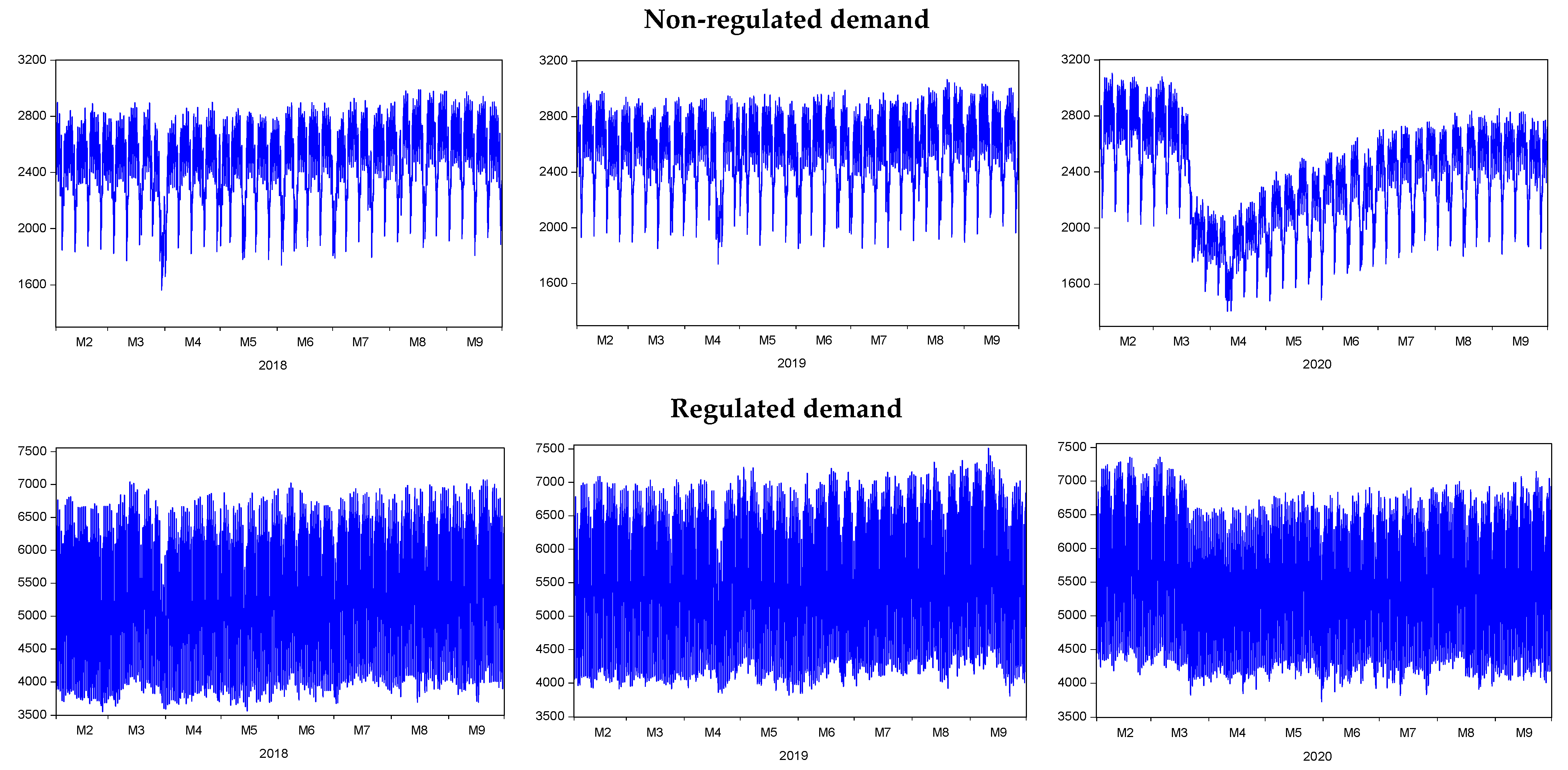
Likewise, Figure 1 presents the non-regulated and regulated demand dynamics for the three study periods: February–September of 2018, 2019, and 2020. According to the authors of [50,54], the annual electricity demand increased by 3.3% between 2017 and 2018. The month of August of 2018 had the highest consumption with 6.02 GWh. Non-regulated demand presented an increase of 5% linked to economic activity growth in 2018. By contrast, regulated demand had an increase of 2.6%. On the other hand, in 2019, electricity consumption was 71.93 GWh, i.e., the electricity demand of the Interconnected National System (INS) increased by 4.02% compared to 2018. Once again, August of 2019 was the month with the highest electricity consumption with 6.26 GWh. The second quarter of 2019 registered the highest demand growth with 4.38% because the non-regulated and regulated market increased by 3.67% and 4.9%, respectively. During 2019, the economic activity had relevant participation over the non-regulated demand dynamic. Industrial participation was 42.65%, and mining exploitation participation was 24.61%; also, both increased their energy consumption by approximately 4%. Therefore, the industrial sector had a strong correlation to the non-regulated demand variability.

However, the growth trend of electricity demand was interrupted by restriction mobility from March 2020. The month of April presented the highest demand decrease, reaching 5.2 GWh, which represented a reduction of 10.7%. On the other hand, in the pre-pandemic months, January and February, there was a growth of 4.9% and 5.0%, respectively. According to the authors of [14,55], the restriction policies in March caused a decrease in non-regulated and regulated demand of 17% and 11%, respectively, compared to the previous month. This was the biggest fall in electricity demand due to a contraction in economic activity. In the coming months, from April to July, recovery was observed, mainly of non-regulated demand, because of the reopening of some economic sectors.

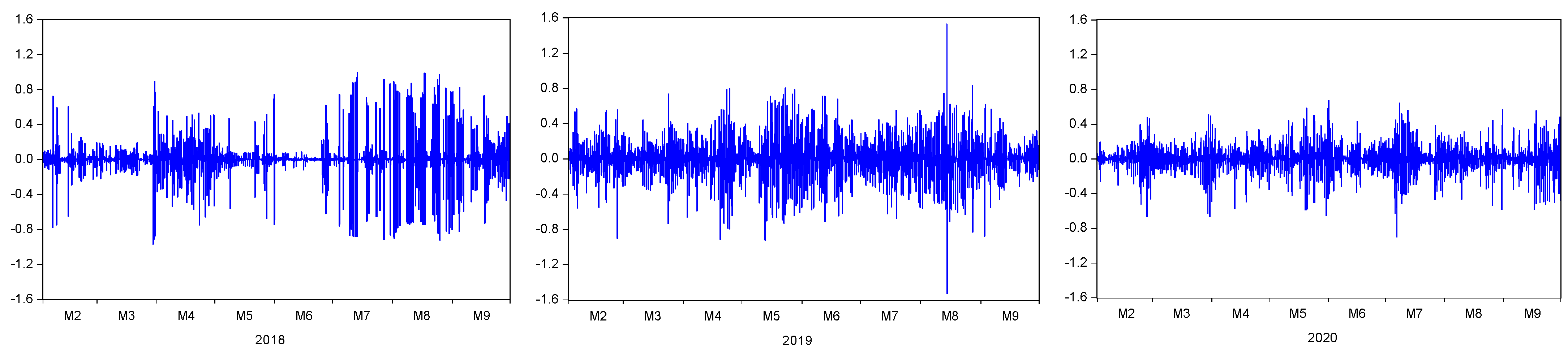
By contrast, electricity demand is one of the most relevant spot price determinants due to the price dynamics that capture the supply and demand variations caused by the technological and organizational aspects of the electricity market [40,56,57]. Figure 2 shows the electricity price returns during the three study periods. During the first semester of 2018, the evolution of the spot price was stable, with values close to 200 COP/kWh, while the second semester showed a high variability due to changes in the hydric sources. Despite the constant price variation during February–September 2019, the hourly spot price reached its highest level, 910.47 COP/kWh, on August 15 at 14:00–15:00 h, which caused the Reliability Charge activation [50,54]. Besides, and according to the authors of [58,59,60], the hydric reservoirs decreased by 50% from December of 2019, reaching a stable level of 35%. Therefore, the thermal power generation increased by 4.8% compared to the same period in 2018. This phenomenon increased the electricity spot price in February 2020. However, electricity demand reduction due to the health emergency caused a monthly spot price decrease of 41% between March and April. During the coming months, the hydric reservoirs were low, and the commercial and industrial sectors’ flexibility caused an increase in the volatility of the spot price. Finally, between June and September, the spot price decreased due to the increase in the water reservoir levels up to 65%, and electricity demand was stable.

4. Empirical Results and Discussion

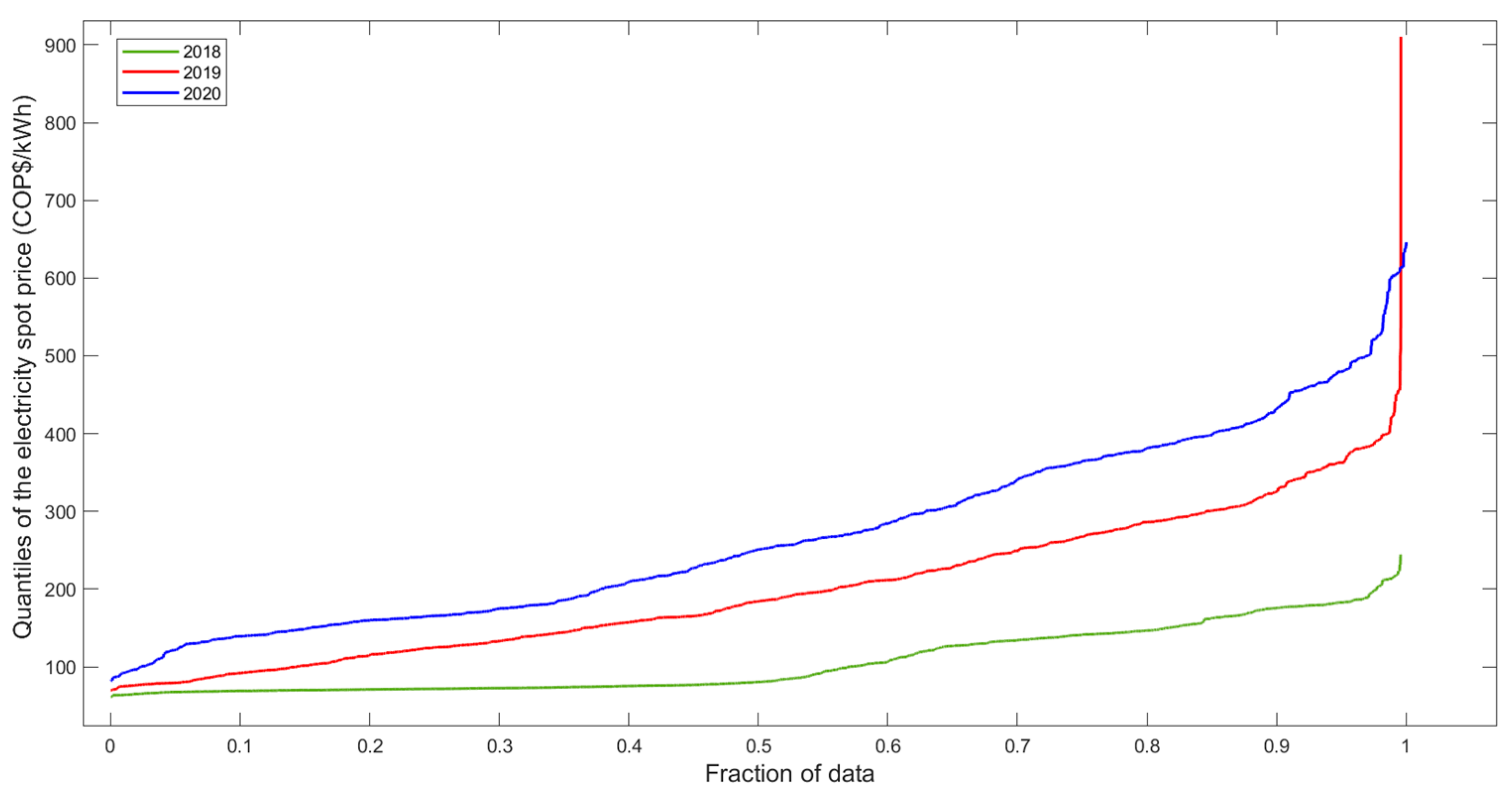
The results of the QR analysis are described below for the percentiles of the electricity price distribution. Figure 3 shows the spot prices’ quantiles against the corresponding fraction of data for the three study periods. The spot price observed in 2020 presented the highest values for each percentile. The lower price was 81.85 COP/kWh due to the increase in the demand shock and in the water reservoirs. Likewise, the median spot price was around 251 COP/kWh, and from the 10th to the 90th quantile, the spot price presented a positive linear trend, similar to 2019; however, after the 90th quantile, the price increased with an exponential dynamic related to the reopening of the economic sectors and the low water levels in reservoirs. For 2019, an extreme value was observed in the last quantile related to a sharp peak value on August 15. For 2018, the prices are described by an average value close to 75 COP/kWh between the 0th and 50th quantile. Nevertheless, after the median, the prices had a smoothy positive trend.

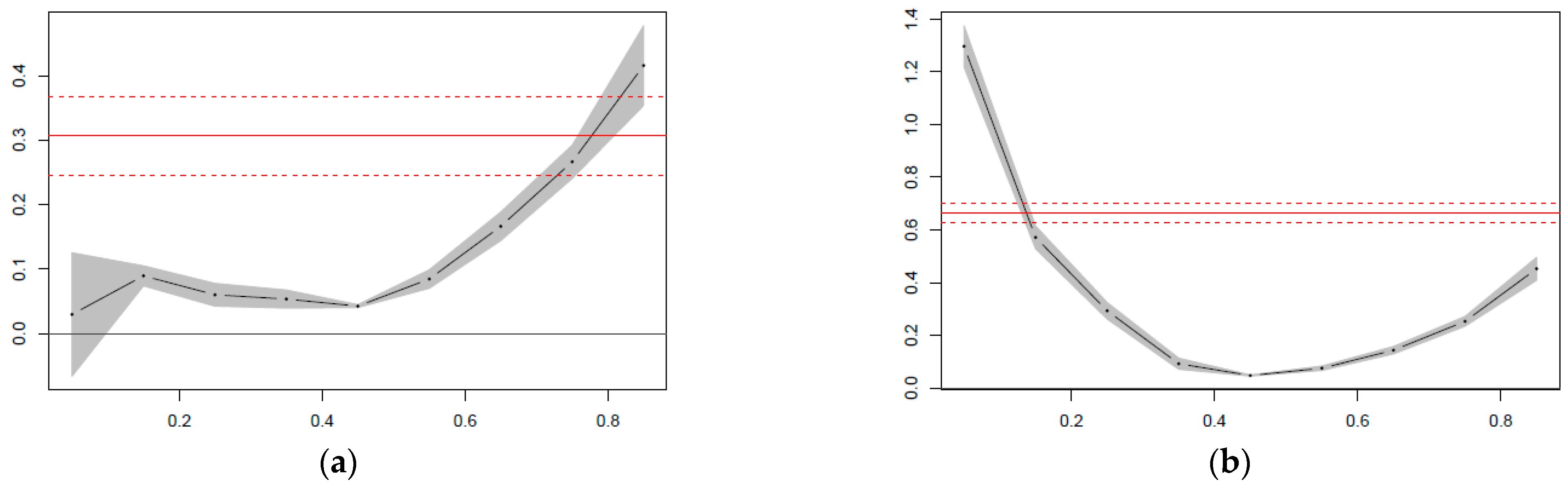
The main findings are summarized in Figure 4, and the QR coefficients are presented in Appendix A. The quantile regression allows the way in which the non-regulated and regulated demand dynamics translated into increments or decrements in the electricity spot price variability to be observed. The analysis of demand is statistically significant for the periods of 2018 and 2020, while for the sample in 2019 in the 20th and 30th percentiles, the non-regulated demand effect was not significant. Moreover, the effects varied over the different spot price quantiles for the three study periods.

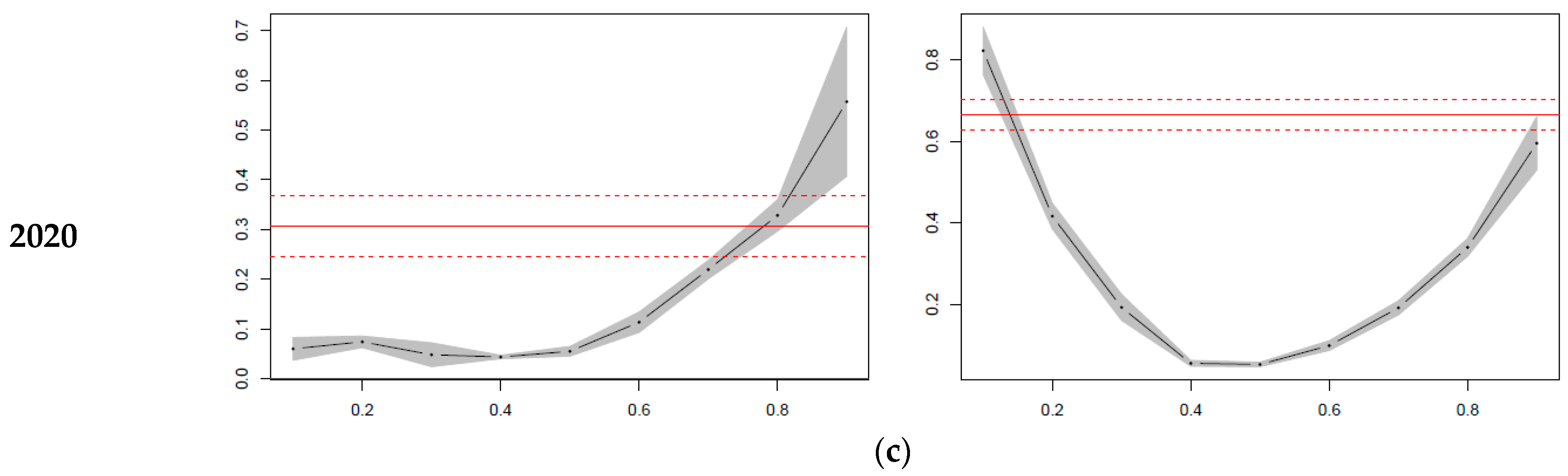
First, based on non-regulated demand, from the 10th to the 40th percentile, the demand presented a low impact, i.e., for a demand variation of 1%, the price showed variability between 0.04% and 0.06% in 2020. Therefore, this effect is associated with the negative demand shock during March and April due to the mobility restriction policies. According to the authors of [34], the spot price showed a monthly growth rate of 25%, the lowest in the last semester. However, as of the 50th percentile, the impact was higher. In the 80th and 90th percentile, the price variability increased by approximately 0.33% and 0.56%, respectively. Therefore, this result is related to the reopening of the economic sectors that increased the non-regulated demand. During May, the interannual growth in spot price was 139% [59]. Despite progressive economic recovery, the non-regulated market did not meet its pre-pandemic level due to the economic sectors with the highest demand participation having negative growth rates: the manufacturing industry grew by −6.52%; mining exploitation by −4.51%; and social, communal, and personal services by −12.84% [61]. In November, the non-regulated demand showed a growth of −3.4%.

On the other hand, the price variation caused by non-regulated demand in 2018 and 2019 presented similar behavior for each percentile. For 2018, the spot price increased its variability in the extreme percentiles. In the 10th percentile, a demand variation of 1% increased the price variability by 0.12%. However, in the 80th and the 90th percentiles, the same demand variation increased the price by 0.17% and 0.44%, respectively. In 2019, the first percentiles were not statistically significant; thus, the most relevant effects can be observed in the higher percentiles, e.g., in the 90th percentile, a demand variation caused a price variation of 0.87%. Therefore, the demand effects were higher in 2019, followed by 2020 and 2018.

Second, the effects of regulated demand were positive and statistically significant for all percentiles in 2020. From the 10th to 20th percentile, where the prices were low, the demand showed a strong positive effect on the price dynamic. With a demand variation of 1%, the price variation increased by approximately 0.82% and 0.42%, respectively. With the percentiles close to the median, the effects were lower. However, from the 70th percentile, the demand effect was higher again. For example, in the higher percentiles, the price variation increased by approximately 0.59%. According to the authors of [61], the regulated market had participation in total demand of 69.96%; thus, this demand caused the highest effect on the spot price variability. These results are similar to 2018 and 2019 because the lower quantiles caused a higher impact on price variability. Nevertheless, an El Niño shock from the end of 2018 to the second semester of 2019 caused the highest variance of the spot price in the sample of 2019 which was higher than 2020 [50]. According to the authors of [6,30,62] negative shocks increase the volatility over the positive shocks. Therefore, the El Niño shock is associated with greater uncertainty and takes longer to be recovered from. These effects are transmitted to tomorrow’s volatility, increasing the price variance.

The findings showed significant effects on the spot price during the strict quarantine. According to the authors of [3,63,64,65], during the COVID-19 pandemic, electricity prices dropped and volatility increased due to a fall in the load demand and consumption changes due to the state of emergency and work-from-home policies in many countries. Electricity demand and consumption are relevant spot price determinants. Besides, a part of the spot price trend can be explained by demand shocks, principally in the short term [66,67,68].

However, in the short term, the demand is inelastic, i.e., it does not show changes by price due to the fact it has a standard curve for each hour of the day and each day of the week. On the other hand, the Colombian regulations allow only one offer and one price per day for each power generator. The supply strategy must be based on the daily complete demand curve, but the market-clearing price shows hourly changes by the demand dynamic. Consequently, the electricity spot price cannot fully capture a demand shock with a short duration because the power generators would not change their strategies, and also, the spot exchanges are accompanied by long-term bilateral contracts to cover a large part of demand with a fixed price. Besides, the Colombian electricity market is based on a hydrothermal power generation market, where the agents have the El Niño shock incorporated in their strategy supply. Therefore, the price dynamic is affected and the risk is high when, e.g., the primary generation source is impacted [40]. Therefore, the price variability was higher in 2019 than in 2020 due to the fact that market agents did not anticipate the effects of the strict quarantine.

Robustness Analysis

The robustness analysis for 2020 was applied by a different choice of quantile range $q$ and a new selection of explanatory variables [43]. First, the coefficients were estimated under (0.05, 0.85) quantile values. The results are presented in Appendix B, in Figure A1 and

Table A4. Quantile regression coefficients for the threshold levels (0.05, 0.85) in 2020.

	${\mathit{\beta }}^{0.1}$	${\mathit{\beta }}^{0.2}$	${\mathit{\beta }}^{0.3}$	${\mathit{\beta }}^{0.4}$	${\mathit{\beta }}^{0.5}$	${\mathit{\beta }}^{0.6}$	${\mathit{\beta }}^{0.7}$	${\mathit{\beta }}^{0.8}$	${\mathit{\beta }}^{0.9}$
Intercept	−0.1181 ***	−0.0394 ***	−0.0148 ***	−0.0027	0.0000 ***	0.0016 ***	0.0057 ***	0.0146 ***	0.0361 ***
Non-regulated demand	0.0299	0.0898 ***	0.0604 ***	0.0538 ***	0.0428 ***	0.0848 ***	0.1665 ***	0.2665 ***	0.4157 ***
Regulated demand	1.2972 ***	0.5715 ***	0.2929 ***	0.0918 ***	0.0470 ***	0.0747 ***	0.1431 ***	0.2528 ***	0.4525 ***

Note: *** indicate the significance levels of 1%.

. Second, the hydraulic and thermal generation capacities were added to model two of the most relevant spot price determinants [40]. Therefore, Equation (4) can be written as:

$$Q_q\left(P_{i,t}\right)={\beta }_{i,1}^q+{\beta }_{i,2}^{q}NR{D}_t+{\beta }_{i,3}^{q}R{D}_t+{\beta }_{i,4}^{q}H{G}_t+{\beta }_{i,5}^{q}T{G}_t,$$

(5)

where, $H{G}_t$ is the generation capacity by hydraulic sources and $T{G}_t$ is the generation capacity by thermal sources. Both variables were observed in kWh, and the results are described in Figure A2 and

Table A5. Quantile regression coefficients for the added explanatory variables.

	${\mathit{\beta }}^{0.1}$	${\mathit{\beta }}^{0.2}$	${\mathit{\beta }}^{0.3}$	${\mathit{\beta }}^{0.4}$	${\mathit{\beta }}^{0.5}$	${\mathit{\beta }}^{0.6}$	${\mathit{\beta }}^{0.7}$	${\mathit{\beta }}^{0.8}$	${\mathit{\beta }}^{0.9}$
Intercept	−0.0648 ***	−0.0242 ***	−0.0086 ***	−0.0007 ***	0.0005 ***	0.0030 ***	0.0093 ***	0.0227 ***	0.0628 ***
Non-regulated demand	0.0720	0.0692 ***	0.0389 ***	0.0307 ***	0.0436 ***	0.1128 ***	0.2430 ***	0.4103 ***	0.6521 ***
Regulated demand	0.8170 ***	0.4096 ***	0.1723 ***	0.0295 ***	0.0303 ***	0.1002 ***	0.2550 ***	0.4883 ***	0.8567 ***
Hydraulic generation	−0.0470	−0.0076	0.0140	0.0247 ***	0.0200 ***	−0.0008	−0.0614 ***	−0.1543 ***	−0.2669 **
Thermal generation	0.1443 ***	0.0536 ***	0.0302 ***	0.0131 ***	0.0079 ***	−0.0031	−0.0234 ***	−0.0343	−0.0153

Note: ** and *** indicate the significance levels of 5% and 1%, respectively.

. The results were similar in comparison with the previous section. Therefore, the interpretation of the results and the conclusion did not change.

5. Conclusions

Electricity demand captures the dynamics of economic activity and transfers its fluctuations into electricity market variables. However, one of the most relevant variables affected by the demand variation is the electricity spot price. Electricity consumption, especially the non-regulated demand decreased significantly between March and April 2020 due to stay-at-home restrictions in Colombia. However, during the coming months, energy consumption started to recover, but it did not achieve the levels observed before the health emergency.

Therefore, a quantile regression analysis was used to identify the effects of regulated and non-regulated electricity demand on the electricity spot price during the period of confinement by COVID-19 disease. The sensitivity analysis showed high variability in the spot price by regulated demand variations during the first months of strict quarantine. The effect was higher in lower spot price percentiles due to the fact that regulated demand increased due to work-from-home policies. Nevertheless, the effect decreased in values close to the median.

On the other hand, the comparative analysis between the three study periods showed similar dynamics. However, in 2019 the spot price had a higher variability since an El Niño shock increases the risk in the generation sector and decreases their benefits. Likewise, the spot price returns during 2020 could not fully capture the effects of non-regulated and regulated demand due to the generation. The market cannot respond to a demand change with a short duration, and the pandemic did not affect the primary generation source, i.e., the water reservoirs. Besides, the action of the bilateral contracts served as a shock absorber.

Finally, the information related to the volatility of the electricity spot price is relevant to energy planning policies. This provides different elements to producers and market agents to anticipate the shocks and improves the energy sector’s response to the risk due to price fluctuations. The limitation of the research is related to the impossibility of observing the post-pandemic situation. Therefore, future research proposals should evaluate the demand effects on electricity prices in the post-pandemic period and identify a possible supply response. Moreover, it would be relevant to analyze the electricity price changes between countries with different generation structures and their response to the COVID-19 shock.

References

1. World Health Organization. Statement on the Second Meeting of the International Health Regulations (2005) Emergency Committee Regarding the Outbreak of Novel Coronavirus (2019-nCoV). Available online: https://www.who.int/news/item/30-01-2020-statement-on-the-second-meeting-of-the-international-health-regulations-(2005)-emergency-committee-regarding-the-outbreak-of-novel-coronavirus-(2019-ncov) (accessed on 6 April 2021).
2. Ayittey, F.K.; Ayittey, M.K.; Chiwero, N.B.; Kamasah, J.S.; Dzuvor, C. Economic impacts of Wuhan 2019-nCoV on China and the world. J. Med. Virol. 2020, 92, 473–475. [Google Scholar] [CrossRef] [Green Version]
3. Zhong, H.; Tan, Z.; He, Y.; Xie, L.; Kang, C. Implications of COVID-19 for the electricity industry: A comprehensive review. CSEE J. Power Energy Syst. 2020, 6, 489–495. [Google Scholar] [CrossRef]
4. Navon, A.; Machlev, R.; Carmon, D.; Onile, A.E.; Belikov, J.; Levron, Y. Effects of the COVID-19 Pandemic on Energy Systems and Electric Power Grids—A Review of the Challenges Ahead. Energies 2021, 14, 1056. [Google Scholar] [CrossRef]
5. Jiang, P.; Fan, Y.V.; Klemeš, J.J. Impacts of COVID-19 on energy demand and consumption: Challenges, lessons and emerging opportunities. Appl. Energy 2021, 285, 116441. [Google Scholar] [CrossRef]
6. Bahmanyar, A.; Estebsari, A.; Ernst, D. The impact of different COVID-19 containment measures on electricity consumption in Europe. Energy Res. Soc. Sci. 2020, 68, 101683. [Google Scholar] [CrossRef]
7. Ghiani, E.; Galici, M.; Mureddu, M.; Pilo, F. Impact on Electricity Consumption and Market Pricing of Energy and Ancillary Services during Pandemic of COVID-19 in Italy. Energies 2020, 13, 3357. [Google Scholar] [CrossRef]
8. Santiago, I.; Moreno-Munoz, A.; Quintero-Jiménez, P.; Garcia-Torres, F.; Gonzalez-Redondo, M.J. Electricity demand during pandemic times: The case of the COVID-19 in Spain. Energy Policy 2021, 148, 111964. [Google Scholar] [CrossRef] [PubMed]
9. IEA Global Energy Review 2020: The Impacts of the COVID-19 Crisis on Global Energy Demand and CO2 Emissions. Available online: https://www.iea.org/reports/global-energy-review-2020 (accessed on 6 April 2021).
10. Norouzi, N.; de Rubens, G.Z.; Choupanpiesheh, S.; Enevoldsen, P. When pandemics impact economies and climate change: Exploring the impacts of COVID-19 on oil and electricity demand in China. Energy Res. Soc. Sci. 2020, 68, 101654. [Google Scholar] [CrossRef] [PubMed]
11. Agdas, D.; Barooah, P. Impact of the COVID-19 Pandemic on the U.S. Electricity Demand and Supply: An Early View from Data. IEEE Access 2020, 8, 151523–151534. [Google Scholar] [CrossRef]
12. Abu-Rayash, A.; Dincer, I. Analysis of the electricity demand trends amidst the COVID-19 coronavirus pandemic. Energy Res. Soc. Sci. 2020, 68, 101682. [Google Scholar] [CrossRef]
13. Carvalho, M.; de Mello Delgado, D.B.; Lima, K.M.; Cancela, M.C.; Siqueira, C.A.; Souza, D.L.B. Effects of the COVID-19 pandemic on the Brazilian electricity consumption patterns. Int. J. Energy Res. 2021, 45, 3358–3364. [Google Scholar] [CrossRef]
14. Vidal, P.; Sierra, L.; Cerón, J. Demanda Nacional de Energía y Crecimiento Económico en Tiempos de Cuarentena; Boletín No 2; Pontificia Univerdiad Javeriana: Cali, Colombia, 2020. [Google Scholar]
15. Yun, Z.; Quan, Z.; Caixin, S.; Shaolan, L.; Yuming, L.; Yang, S. RBF neural network and ANFIS-based short-term load forecasting approach in real-time price environment. IEEE Trans. Power Syst. 2008, 23, 853–858. [Google Scholar] [CrossRef]
16. Karakatsani, N.V.; Bunn, D.W. Forecasting electricity prices: The impact of fundamentals and time-varying coefficients. Int. J. Forecast. 2008, 24, 764–785. [Google Scholar] [CrossRef]
17. Bierbrauer, M.; Menn, C.; Rachev, S.T. Spot and derivative pricing in the EEX power market q. J. Bank. Financ. 2007, 31, 3462–3485. [Google Scholar] [CrossRef]
18. Aggarwal, S.K.; Saini, L.M.; Kumar, A. Electricity price forecasting in deregulated markets: A review and evaluation. Int. J. Electr. Power Energy Syst. 2009, 31, 13–22. [Google Scholar] [CrossRef]
19. Huisman, R.; Mahieu, R. Regime jumps in electricity prices. Energy Econ. 2003, 25, 425–434. [Google Scholar] [CrossRef] [Green Version]
20. Weron, R.; Przybyłowicz, B. Hurst analysis of electricity price dynamics. Phys. Stat. Mech. Its Appl. 2000, 283, 462–468. [Google Scholar] [CrossRef] [Green Version]
21. Ketterer, J.C. The impact of wind power generation on the electricity price in Germany. Energy Econ. 2014, 44, 270–280. [Google Scholar] [CrossRef] [Green Version]
22. Rafiei, M.; Niknam, T.; Khooban, M.-H. Probabilistic Forecasting of Hourly Electricity Price by Generalization of ELM for Usage in Improved Wavelet Neural Network. IEEE Trans. Ind. Inform. 2017, 13, 71–79. [Google Scholar] [CrossRef]
23. Mujeeb, S.; Javaid, N.; Ilahi, M.; Wadud, Z.; Ishmanov, F.; Afzal, M.K. Deep long short-term memory: A new price and load forecasting scheme for big data in smart cities. Sustain. Switz. 2019, 11, 987. [Google Scholar] [CrossRef] [Green Version]
24. Demir, S.; Mincev, K.; Kok, K.; Paterakis, N.G. Introducing technical indicators to electricity price forecasting: A feature engineering study for linear, ensemble, and deep machine learning models. Appl. Sci. Switz. 2020, 10, 255. [Google Scholar] [CrossRef] [Green Version]
25. Weron, R. Electricity price forecasting: A review of the state-of-the-art with a look into the future. Int. J. Forecast. 2014, 30, 1030–1081. [Google Scholar] [CrossRef] [Green Version]
26. Nowotarski, J.; Weron, R. Recent advances in electricity price forecasting: A review of probabilistic forecasting. Renew. Sustain. Energy Rev. 2018, 81, 1548–1568. [Google Scholar] [CrossRef]
27. Hinderks, W.J.; Wagner, A. Factor models in the German electricity market: Stylized facts, seasonality, and calibration. Energy Econ. 2020, 85, 104351. [Google Scholar] [CrossRef]
28. Lisi, F.; Shah, I. Forecasting next-day electricity demand and prices based on functional models. Energy Syst. 2020, 11, 947–979. [Google Scholar] [CrossRef]
29. AleaSoft Historical Fall in Demand and Prices of the European Electricity Markets in April. Available online: https://aleasoft.com/historical-fall-demand-prices-european-electricity-markets-april/ (accessed on 8 April 2021).
30. Norouzi, N.; de Rubens, G.Z.; Enevoldsen, P.; Forough, A.B. The impact of COVID-19 on the electricity sector in Spain: An econometric appr oach based on prices. Int. J. Energy Res. 2021, 45, 6320–6332. [Google Scholar] [CrossRef]
31. Ghanem, S.; Fandi, G.; Krepl, V.; Husein, T.; Rzek, O.; Muller, Z.; Kyncl, J.; Tlustý, J.; Smutka, L. The Impact of COVID-19 on Electricity Prices in Italy, the Czech Republic, and China. Appl. Sci. 2021, 11, 8793. [Google Scholar] [CrossRef]
32. Figueroa, J.; Counts, T.; Graves, F.; Mudge, B.; Pant, S. Impact of COVID-19 on the US Energy Industry; The Brattle Group: Cambridge, MA, USA, 2020; Available online: https://brattlefiles.blob.core.windows.net/files/18557_impact_on_covid-19_on_the_us_energy_industry.pdf (accessed on 30 September 2021).
33. Murty, V.V.S.N.; Sharme, A.K. Impact of COVID’19 Pandemic on Indian Electrical Distribution system. Int. J. Comput. Digit. Syst. 2020, 10, 1–11. [Google Scholar]
34. UPME. Inflación de Energía en Colombia: Abril 2020; Minenergía: Bogotá, Colombia, 2020. [Google Scholar]
35. Hallack, M.; Weiss, M. Electricity prices: The heterogeneous impact of COVID-19 on LAC markets. Energ. Para El Futuro 2020. [Google Scholar]
36. Egger, D.; Miguel, E.; Warren, S.S.; Shenoy, A.; Collins, E.; Karlan, D.; Parkerson, D.; Mobarak, A.M.; Fink, G.; Udry, C.; et al. Falling living standards during the COVID-19 crisis: Quantitative evidence from nine developing countries. Sci. Adv. 2021, 7, eabe0997. [Google Scholar] [CrossRef]
37. Reyes Ortiz, G.E.; Mendoza-Sáenz, C.A.; Robayo-Piñeros, E.L. Países de la Alianza del Pacífico 2000-2021: Efectos del COVID-19 en el crecimiento y la reactivación económica. Rev. Finanz. Política Económica 2021, 13, 99–113. [Google Scholar] [CrossRef]
38. CREG. Medidas Transitorias Para el Pago de las Tarifas de Energía Eléctrica; Comisión de Regulación de Enegía y Gas: Bogotá, Colombia, 2020; pp. 1–18. [Google Scholar]
39. Mosquera-López, S.; Manotas-Duque, D.F.; Uribe, J.M. Risk asymmetries in hydrothermal power generation markets. Electr. Power Syst. Res. 2017, 147, 154–164. [Google Scholar] [CrossRef]
40. Oviedo-Gómez, A.; Londoño-Hernández, S.M.; Manotas-Duque, D.F. Electricity price fundamentals in hydrothermal power generation markets using machine learning and quantile regression analysis. Int. J. Energy Econ. Policy 2021, 11, 66–77. [Google Scholar] [CrossRef]
41. Cotia, B.P.; Borges, C.L.T.; Diniz, A.L. Optimization of wind power generation to minimize operation costs in the daily scheduling of hydrothermal systems. Int. J. Electr. Power Energy Syst. 2019, 113, 539–548. [Google Scholar] [CrossRef]
42. Ma, L.; Koenker, R. Quantile regression methods for recursive structural equation models. J. Econom. 2006, 134, 471–506. [Google Scholar] [CrossRef] [Green Version]
43. Maciejowska, K. Assessing the impact of renewable energy sources on the electricity price level and variability—A quantile regression approach. Energy Econ. 2020, 85, 104532. [Google Scholar] [CrossRef]
44. Uribe, J.M.; Guillen, M. Quantile Regression for Cross-Sectional and Time Series Data: Applications in Energy Markets Using R; Springer Briefs in Finance; Springer International Publishing: Cham, Switzerland, 2020; ISBN 978-3-030-44503-4. [Google Scholar]
45. Wang, Y.; Zhang, H.; Gao, W.; Yang, C. COVID-19-related government interventions and travel and leisure stock. J. Hosp. Tour. Manag. 2021, 49, 189–194. [Google Scholar] [CrossRef]
46. Bonacini, L.; Gallo, G.; Scicchitano, S. Working from home and income inequality: Risks of a ‘new normal’ with COVID-19. J. Popul. Econ. 2021, 34, 303–360. [Google Scholar] [CrossRef]
47. Azimli, A. The impact of COVID-19 on the degree of dependence and structure of risk-return relationship: A quantile regression approach. Finance Res. Lett. 2020, 36, 101648. [Google Scholar] [CrossRef] [PubMed]
48. Narayan, P.K.; Gong, Q.; Ahmed, H.J.A. Is there a pattern in how COVID-19 has affected Australia’s stock returns? Appl. Econ. Lett. 2021, 1–4. [Google Scholar] [CrossRef]
49. Iqbal, S.; Bilal, A.R.; Nurunnabi, M.; Iqbal, W.; Alfakhri, Y.; Iqbal, N. It is time to control the worst: Testing COVID-19 outbreak, energy consumption and CO2 emission. Environ. Sci. Pollut. Res. 2021, 28, 19008–19020. [Google Scholar] [CrossRef]
50. XM. Reporte Integral de Sostenibilidad, Operación y Mercado 2019; XM: Medellín, Antioquia, Colombia, 2020; pp. 1–187. [Google Scholar]
51. Koenker, R. Quantile regression for longitudinal data. J. Multivar. Anal. 2004, 91, 74–89. [Google Scholar] [CrossRef] [Green Version]
52. Koenker, R.; Bassett, G. Regression Quantiles. Econometrica 1978, 46, 33. [Google Scholar] [CrossRef]
53. Mosquera-López, S.; Uribe, J.M.; Manotas-Duque, D.F. Nonlinear empirical pricing in electricity markets using fundamental weather factors. Energy 2017, 139, 594–605. [Google Scholar] [CrossRef]
54. XM. Reporte Integral de Sostenibilidad, Operación y Mercado 2018; XM: Medellín, Antioquia, Colombia, 2019; pp. 1–381. [Google Scholar]
55. Vidal, P.; Sierra, L.; Cerón, J. Señales en la Demanda de Energía en la Fase de Desconfinamiento.; Boletín No 7; Pontificia Univerdiad Javeriana: Cali, Colombia, 2020. [Google Scholar]
56. Díaz-Contreras, J.A.; Macías-Villalba, G.I.; Luna-González, E. Estrategia de cobertura con productos derivados para el mercado energético colombiano. Estud. Gerenciales 2014, 30, 55–64. [Google Scholar] [CrossRef] [Green Version]
57. Girish, G.P.; Vijayalakshmi, S. Determinants of Electricity Price in Competitive Power Market. Int. J. Bus. Manag. 2013, 8, 70–75. [Google Scholar] [CrossRef] [Green Version]
58. UPME. Inflación de Energía en Colombia: Marzo 2020; Minenergía: Bogotá, Colombia, 2020. [Google Scholar]
59. UPME. Inflación de Energía en Colombia: Mayo 2020; Minenergía: Bogotá, Colombia, 2020. [Google Scholar]
60. UPME. Inflación de Energía en Colombia: Agosto 2020; Minenergía: Bogotá, Colombia, 2020. [Google Scholar]
61. XM. Reporte Integral de Sostenibilidad, Operación y Mercado 2020; XM: Medellín, Antioquia, Colombia, 2021; pp. 1–323. [Google Scholar]
62. Kuzemko, C.; Bradshaw, M.; Bridge, G.; Goldthau, A.; Jewell, J.; Overland, I.; Scholten, D.; Van de Graaf, T.; Westphal, K. Covid-19 and the politics of sustainable energy transitions. Energy Res. Soc. Sci. 2020, 68, 101685. [Google Scholar] [CrossRef]
63. Tashpulatov, S.N. Modeling and Estimating Volatility of Day-Ahead Electricity Prices. Mathematics 2021, 9, 750. [Google Scholar] [CrossRef]
64. Xu, A.T.; Gao, B.W.; Li, C.Y.; Qian, D.F. Impact of the COVID-19 pandemic on the reduction of electricity demand and the integration of renewable energy into the power grid. J. Renew. Sustain. Energy 2021, 13, 026304. [Google Scholar] [CrossRef]
65. Abadie, L.M. Energy Market Prices in Times of COVID-19: The Case of Electricity and Natural Gas in Spain. Energies 2021, 14, 1632. [Google Scholar] [CrossRef]
66. Barrientos, J.; Rodas, E.; Velilla, E. Modelo para el pronóstico del precio de la energía eléctrica en Colombia. Lect. Econ. 2012, 91–127. [Google Scholar]
67. Barrientos-Marín, J.; Toro-Martínez, M. Análisis de los fundamentales del precio de la energía eléctrica: Evidencia empírica para Colombia. Rev. Econ. Caribe 2017, 34–63. [Google Scholar] [CrossRef]
68. García, J.; Gaviria, A.; Salazar, L. Determinantes del precio de la energía eléctrica en el mercado no regulado en Colombia. Cienc. Estratégicas 2011, 19, 225–246. [Google Scholar]
Figure 1. Evolution of the electricity demands for February–September of 2018–2019–2020.
Energies 14 06989 g001
Figure 2. Logarithmic returns of the electricity spot prices for February–September of 2018–2019–2020.
Energies 14 06989 g002
Figure 3. Quantiles’ electricity spot prices for February–September of 2018–2019–2020.
Energies 14 06989 g003
Figure 4. Non-regulated and regulated demand effects on the electricity spot price for different percentiles and for February–September of 2018–2019–2020. The variables are defined as follows: (a) effects of the non-regulated and regulated demand in 2018; (b) effects of the non-regulated and regulated demand in 2019; (c) effects of the non-regulated and regulated demand in 2020. The vertical axis in each subplot corresponds to the spot price response by effects of the demand variables, and the horizontal axis corresponds to each percentile. The dotted black lines represent the quantile regression coefficients, and the gray shaded area is the 95% confidence interval. The continuous red line is the linear regression coefficient estimated by OLS, and the discontinuous red lines are the 95% confidence intervals.
Energies 14 06989 g004aEnergies 14 06989 g004b