Article

A Crew Scheduling Model to Incrementally Optimize Workforce Assignments for Offshore Wind Farm Constructions

by
Daniel Rippel
1,2,*,
Fatemeh Abasian Foroushani
2,
Michael Lütjen
1 and
Michael Freitag
1,2
1
BIBA—Bremer Institut für Produktion und Logistik GmbH, University of Bremen, Hochschulring 20, 28359 Bremen, Germany
2
Faculty of Production Engineering, University of Bremen, Badgasteiner Str. 1, 28359 Bremen, Germany
*
Author to whom correspondence should be addressed.
Energies 2021, 14(21), 6963; https://doi.org/10.3390/en14216963
Submission received: 14 September 2021 / Revised: 18 October 2021 / Accepted: 19 October 2021 / Published: 22 October 2021
(This article belongs to the Section A3: Wind, Wave and Tidal Energy)

Abstract

:
In the literature, different authors attribute between 15% to 30% of a wind farm’s costs to logistics during the installation, e.g., for vessels or personnel. Currently, there exist only a few approaches for crew scheduling in the offshore area. However, current approaches only satisfy subsets of the offshore construction area’s specific terms and conditions. This article first presents a literature review to identify different constraints imposed on crew scheduling for offshore installations. Afterward, it presents a new Mixed-Integer Linear Model that satisfies these crew scheduling constraints and couples it with a scheduling approach using a Model Predictive Control scheme to include weather dynamics. The evaluation of this model shows reliable scheduling of persons/teams given weather-dependent operations. Compared to a conventionally assumed full staffing of vessels and the port, the model decreases the required crews by approximately 50%. Moreover, the proposed model shows good runtime behavior, obtaining optimal solutions for realistic scenarios in under an hour.

Graphical Abstract

1. Introduction

Wind energy offers an opportunity to satisfy the world’s need for green and sustainable energy. Studies show that the last decade witnessed an exponential increase in produced wind energy [1]. This increase results from more capable turbines [2] and continuously increasing concurrent installation and refurbishing projects [3]. Offshore wind farms can produce higher amounts of energy when compared to their onshore counterparts, resulting from the ability to install larger turbines and wind farms and higher wind exposure at the open sea [4]. The current political landscape implies that these trends will continue over the following years. In 2020, several countries worldwide reworked their climate policies, potentially resulting in a worldwide reduction of 47% of global emissions by 2050, e.g., banning fossil energy generation or fuel [1].
While offshore wind farms provide large amounts of energy, their installation imposes additional challenges. While higher wind speeds and quickly changing weather conditions at the open sea favor energy generation, they render the installation complicated and impede installation operations in more than a hundred meters of height. Moreover, offshore construction sites allow larger farms but render them harder to reach, requiring precise operations planning using weather forecasts and human experience. Besides these planning-related challenges, the installation of offshore wind farms requires highly specialized equipment and certified personnel. For example, installation vessels, so-called jack-up vessels, usually provide the ability to mount themselves onto the sea bed to stabilizes themselves for crane operations. In various countries, personnel requires special certification and training for offshore installations in such heights. Several authors in the literature estimate logistics costs during the installation phase to make up approximately 15–30% of an offshore wind farm’s lifetime costs [5,6]. Charter costs for vessels, storage spaces, and personnel make up a significant fraction of these costs.
Over the last few years, several authors have proposed models for the planning and scheduling of offshore operations to reduce these costs. The majority of these models aim to estimate the project duration or schedule using historical weather data and, thus, provide decision support on the strategic level. Recent models aim to support the operative installation process by using current weather data and integrate forecasts to generate short- to mid-term plans. Nevertheless, none of the models regard personnel in their planning, and all of them assume that crews are available 24/7. Similarly, several models for the so-called crew scheduling exist, which partially apply to offshore installation projects. Nevertheless, these models only consider a subset of required constraints, e.g., differentiating between vessels and project crews.
Consequently, this article aims to provide a dedicated model for the crew scheduling/workforce management for offshore installation projects. Therefore, the article’s next section presents a literature review that determines general terms and conditions imposed on the workforce management in this domain and identifies existing approaches that might be applicable. The section closes by comparing identified approaches with the imposed terms. Afterward, the article presents the proposed model as an extension of existing models and its integration with the aforementioned operative scheduling approach (which this introduction will describe later in more detail). The following section then evaluates the proposed model/approach regarding its planning quality and computational requirements. Finally, the article closes with a conclusion and outlook.

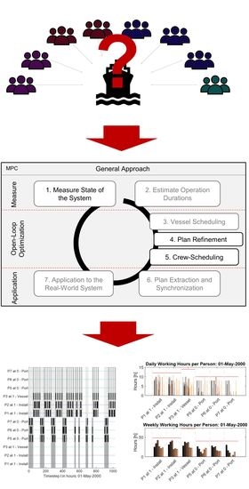
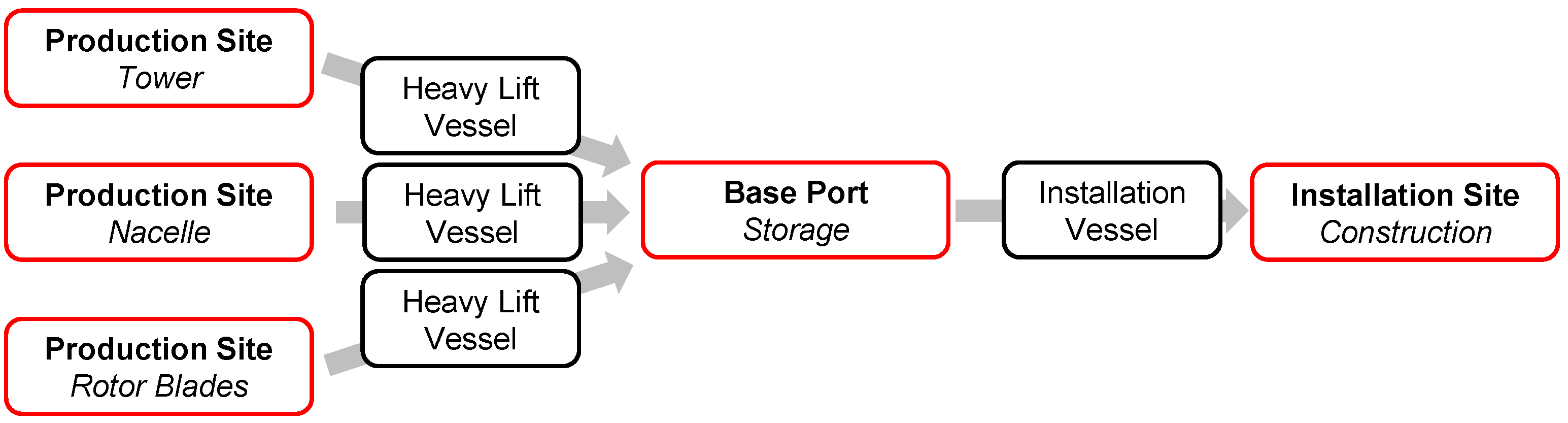
2. Process Description

The literature describes several installation concepts for offshore wind farms: For example, feeder-based concepts [7], pre-assembly concepts [8], or floating concepts where each turbine gets assembled port-side and dragged to the wind farm. Despite this variety, research and practice primarily focus on the so-called conventional installation concept, which is already well established and, e.g., described in Oelker et al. [9]. This concept assumes that dedicated production sites or ports manufacture the main components, i.e., the foundations and cables, the tower (-segments), the nacelle and hub, and the blades. Common heavy-lift transport vessels pick up these components and deliver them to the so-called base port. The base port acts as a decoupling point for this supply chain and buffers component sets for the actual installation. Afterward, a jack-up vessel moves back and forth between the base port and the construction site, picking up several sets and installing the turbines or foundations. Figure 1 depicts this supply chain and the involved vessels for installing turbines.
As noted above, the same supply chain applies to founding structures and top structures/turbines. Nevertheless, both activities require specialized tools on the jack-up vessel. For example, installing founding structures might require so-called hydro-hammers, while installing top structures requires heavy-duty cranes, equipment to work in great heights, and large free deck areas for transporting components. According to Vis and Ursavas [8], companies usually perform these activities sequentially to reduce set-up times and efforts. Therefore, they first install all foundations, then install the top structures, and, finally, perform the commissioning as a third stage. Accordingly, this article focuses on the second stage, the installation of top structures, as this stage involves more components and jobs to be handled by a single vessel. Nevertheless, the proposed models and approaches apply to the first stage without limitations.
The installation of a turbine follows a sequential process. First, the vessel loads as many sets of components as planned for the current installation cycle. Loading and securing a complete set of components takes several hours, depending on the vessel’s capacity up to 12 h. Then, the vessel moves out to the installation site, which, depending on the distance, again can take several hours. The vessel performs the following sequence of operations at the installation site for each loaded set of components. First, it positions itself close to the foundation before commencing its jack-up operation. Afterward, the project crew assembles the turbine bottom-up, i.e., the tower (-segments), the nacelle and hub, and finally, the three blades. Finally, the vessel jacks down again and either repeats this process or returns to the base port. It has to be noted that the vessel will remain in its jack-up state until the turbine has been assembled. Each jack-up operation punctures the sea bed and destabilizes it. Consequently, additional jack-ups at similar locations would put the vessel, its crew, and the already installed components at a high risk of damage.
Due to safety regulations, the crew can only conduct each assembly operation if the current weather conditions do not exceed given limits considering the maximum wave height and wind speed. While the literature lists several different limits for these values, this article uses the limits already applied in previous work, e.g., Reference [10], summarized in Table 1. These values resulted from interviews and simulation studies conducted as part of a previous research project. Rippel et al. [11] list several other limitations given in the literature.
Each operation requires that the wind speed and wave height remain below the given threshold for the entire operation time (base duration). If current values exceed these limits, the crew needs to abort the operation, secure the component and restart when the weather has calmed down. Consequently, operations only start if the crew expects a viable weather window. As the jack-up vessel remains stationary until the installation finishes, quickly changing weather conditions at sea can incur high waiting times and, accordingly, high costs for delayed operations.

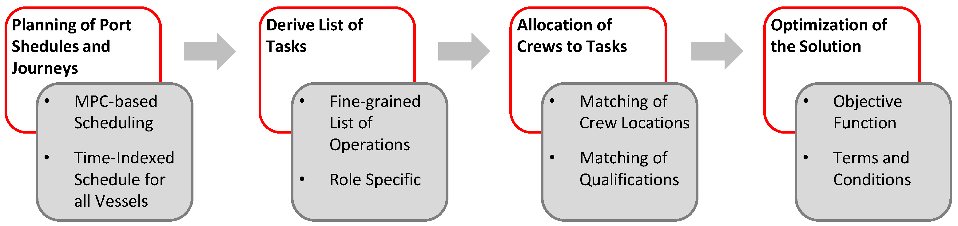
2.1. Planning and Scheduling of Offshore-Operations

As jack-up vessels impose the highest carter costs for offshore constructions, most of the literature in this domain focuses on optimizing installation operations. Over the last decade, several authors proposed mathematical optimization models, e.g., References [12,13,14,15,16,17]. Other authors proposed simulation models, viable to extract suitable schedules for the vessels using different decision strategies or focusing on different additional concepts, such as installation concepts or information sharing, e.g., References [7,8,18,19,20,21]. These models use historical data to create probability distributions for probable weather conditions or follow historical recordings to simulate the project. Consequently, all noted models mainly provide decision support on a strategic level, supporting the advanced planning, but do not include current data needed for operative support.
In contrast, some authors have also proposed models for operative decision support during the last few years. For example, Peng et al. [22] propose a simulation model using timed Petri-nets to select optimal installation cycles using current weather forecasts. Rippel et al. [10] propose an online scheduling approach using Mixed-Integer Linear Programming combined with a Model Predictive Control (MPC) scheme to achieve optimal short-term schedules using current forecasts and weather measurements. This approach consists of an online simulation that tethers into the real-world process, collecting relevant information, such as weather measurements and forecasts, vessel states, and the currently installed wind farm and base port states. The simulation then triggers the optimization whenever a vessel requires a new plan. The optimizer then calculates an optimal plan for P many planning horizons of T many hours, extracts the first period, and relays it back to the simulation and real-world system. The approach relies on an estimation of the duration for future operations using current forecasts and either a sliding window or Markov-Chain-based approach. This estimation allows the optimizer to estimate how much waiting time an operation would include if it commences at a particular hour.

2.2. Conclusion and Research Gap

As can be seen from Table 1, an installation cycle for a vessel with a capacity of four sets takes at least 132 h, i.e., five and a half days. This calculation assumes that no delays occur and the crews work for 24 h a day, each day of the week. Moreover, the table shows that at least three types of crews perform activities during the installation: port-side crews for loading components, vessel crews to operate the installation vessel, and project crews for the assembly. All articles proposing models for the decision support for offshore wind farm installations assume a complete availability of crews to ensure the possibility of working at any time. Nevertheless, each crew only takes over particular operations, and weather-induced delays may add additional down-times. Consequently, this assumption will likely result in an over-staffing of the vessel and the port, resulting in high additional personnel costs. Following this hypothesis, the remainder of this article investigates models for a dedicated crew scheduling for offshore constructions. Furthermore, it presents an option for integrating the crew scheduling with the presented online scheduling approach, enabling operative decision support.

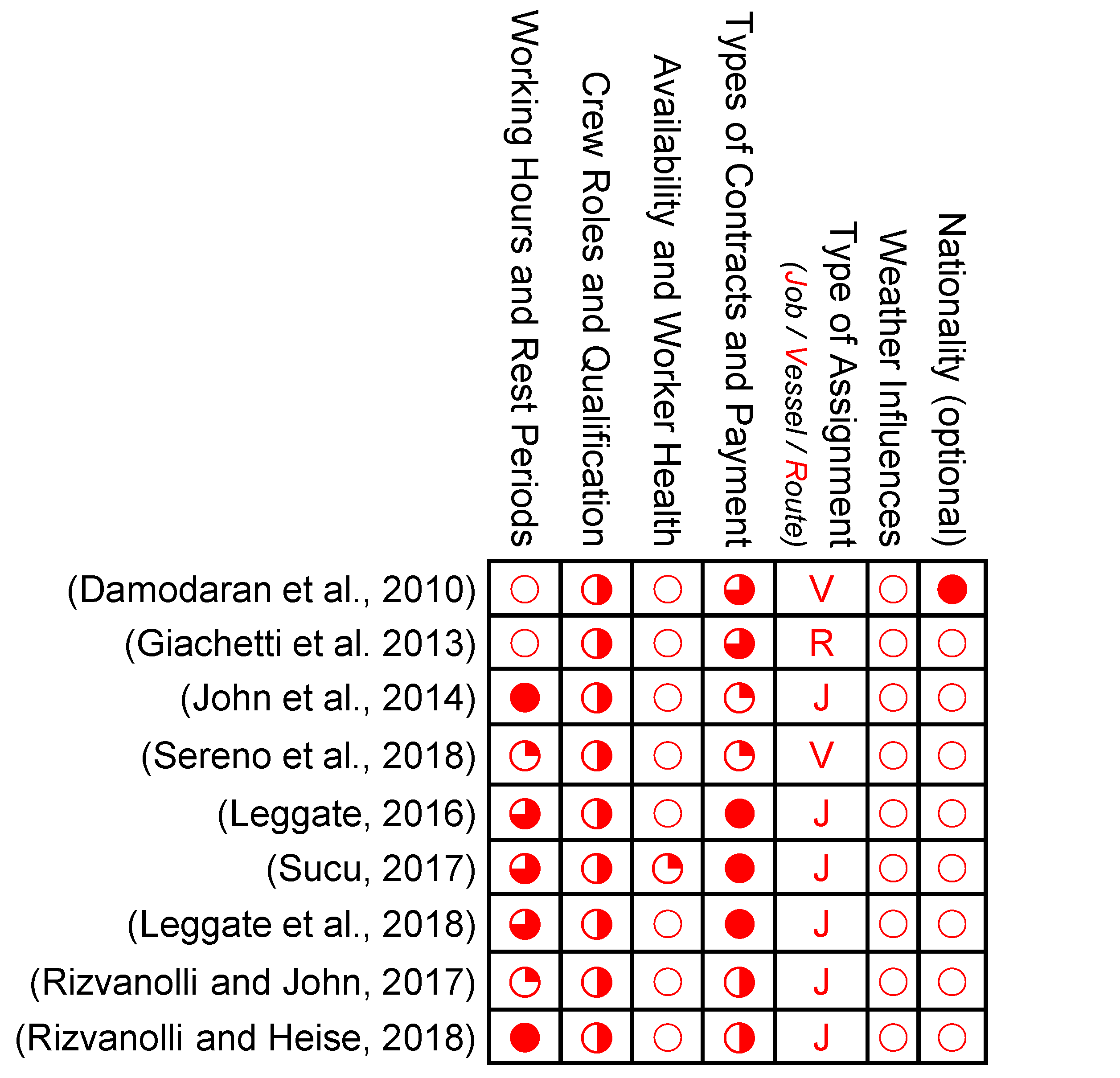
3. Literature Review and Requirements Analysis

This article relies on a structured literature review using the Prisma procedure model [23]. First, this review aims to determine relevant terms and conditions applying to the workforce management for offshore constructions. For example, such conditions include legislative restrictions for working hours, rest periods or maximal times at sea, qualification requirements, and general terms, such as weather dependencies. Second, the review results in a list of existing crew scheduling approaches for the offshore area. The following section, “Workforce-Management Framework”, relies on analyzing these approaches to construct a crew scheduling model that satisfies the identified terms and conditions by extending existing models.
The literature review focused on combinations of the terms personnel planning, human resource planning, crew scheduling, staff scheduling, offshore installation, maritime, and vessel. Moreover, the search included additional synonyms of these terms and their German counterparts. It used various search engines, e.g., Google Scholar, Scopus, ScienceDirect, ResearchGate, or the search engine of Germany’s Federal and University Libraries. Following the Prisma procedure, the review first conducted a search using these terms in various combinations. This initial engine and snow-ball search resulted in 1126 articles and legislative texts in total. The following step (screening of title, abstract, conclusions, and keywords) and limiting the results to articles published over the last twenty years excluded 1007 of these articles. The majority of these articles do not fit the targeted domain or planning problem.
Most of these articles propose qualitative studies, e.g., on worker welfare, do not propose actual models or target unrelated domains. Consequently, the review included 119 articles for the full-text analysis. Twenty-seven of these articles showed relevance for the identification of terms and conditions regarding offshore wind farm constructions. Nevertheless, only nine articles propose models with similar problem statements to support crew scheduling for offshore installations. Most of the excluded articles propose models that focus on other types of personnel planning, e.g., routing or pairing. The remainder of this section discusses these nine articles. Moreover, it discusses the investigated scheduling problem compared to those approaches excluded in the final step. Finally, this section summarizes the terms and conditions identified from analyzing those 27 relevant articles. These results align with previous reviews, e.g., References [24,25]. The topics of personnel and crew scheduling have a long history of publications, but very few works deal with the offshore area in general, and even less with offshore constructions.

3.1. Description of the Investigated Crew Scheduling Problem

The literature review shows the need for an explicit characterization and differentiation of crew scheduling for offshore installations, e.g., compared to crew scheduling in air-, rail, or sea transport, or even compared to the cruise sector.
In the context of this work, crew scheduling aims to assign capable crews or persons ( P ) to a given set of tasks or jobs ( J ), while abiding by applicable terms and conditions, as noted above. For example, the model ensures that personnel is available and located at the right vessel and adheres to working time and rest restrictions. Depending on the interpretation of the overall problem, offshore-crew scheduling could resemble two types of problems: First, when combining the planning of operations and personnel into a single model, the problem constitutes a multi-resource job shop scheduling problem. Second, if separating these steps, the problem reduces to a classical assignment/scheduling problem, i.e., which person or crew takes over which operation.
As described later, this article follows the latter strategy: The proposed framework first obtains an optimal plan for each vessel, denoting which operation should start and finish at which point in time. This plan mainly minimizes vessels’ makespan and associated costs, which inflict the highest costs [10]. Afterward, this article applies the proposed crew scheduling model, minimizing the number of crews or persons required to satisfy this plan. Most articles follow a similar approach and assume fixed operations or trips for the crew scheduling. John et al. [26] propose a procedure that applies to the proposed framework and fairly well describes the extensions needed for the MPC-based scheduling approach (Figure 2).

3.2. Requirement-Analysis

This subsection presents and categorizes the terms and conditions identified by evaluating the 27 articles and legal text resulting from the review and the application domain. Thereby, different authors apply varying subsets of terms and conditions to their models or use different terminologies. Nevertheless, the review shows a total of seven categories of conditions.
Working hours and rest periods: International and national laws impose strict regulations on working hours and rest periods that the crew scheduling needs to satisfy. These regulations differ, e.g., for national, European, or international laws, and are highly dependent on the country the vessel sails for or the crew aboard. Moreover, a single vessel might need to cover different rules for different types of personnel. For example, German laws differ between the actual vessel crew and crews that perform “offshore duties”, i.e., in the case of this article, the project crews [27,28]. Generally, these laws define maximum workloads per day and week, minimum pause and rest periods, and often the maximum time persons can spend offshore. Accordingly, this requirement states that the crew scheduling should handle different sets of rules for a single vessel, preferably defined for each person or crew.
Crew Roles and Qualification: Most of the literature refers to personnel qualification in one way or another. These qualifications range from basic assignments (the person can do a job or not), i.e., the definition of crew roles, to more sophisticated levels of qualification that the optimizer needs to satisfy for each job. Accordingly, each model should at least allow a binary assignment of required and offered roles for jobs and personnel. As this article assumes a fixed sequence of jobs for crew scheduling, the models should also ensure that each job’s minimum qualification level can be guaranteed. Underqualification might result in delays that interfere with the given plan.
In addition to these operative qualification requirements, the literature presents various required qualifications that planners need to regard on the strategic or tactical planning levels. For example, various countries require offshore construction personnel to periodically acquire specific certificates [29]. Moreover, offshore wind farm constructions require highly trained personnel [30], which also influences later requirements, e.g., regarding the payment or the availability in case of unplanned unavailabilities.
Availability and Worker Health: As noted above, a single installation cycle with an average vessel takes about one week before the vessel returns to the base port. Consequently, worker availability and unplanned interruptions due to sickness can severely influence the installation or induce additional costs for crew transfers. Several authors highlight the rough working conditions at sea, which induce a high risk of accidents or additional risks of sickness due to the confined living situation on a vessel [29,30]. Accordingly, this requirement states that crew scheduling for offshore constructions should offer a mechanism to deal with this highly unpredictable situation by imposing monitoring and replanning strategies or applying robust planning approaches.
Types of Contract and Payment: This requirement ties into previous requirements but extends them by costing. Besides inherently different payments and contract conditions for different crew roles, some authors highlight the ability to book additional personnel on short notice. For example, Leggate et al. [31] differentiate between regular and agency personnel, whereby they use the latter to fill in for higher, unplanned demands at higher costs. Accordingly, this requirement states that each model should allow a specification of different costs per person or crew. Optionally, they should allow the integration of agency crews if requested by the planner.
Type of Assignment: As noted above, the type of assignment between personnel, jobs, routes, or vessels imposes a significant requirement for the viability of models in offshore constructions. While most crew scheduling models assign personnel to single vessels or routes (pairing), the article at hand requires the assignment of personnel to single jobs during each trip.
Influence of Weather and Forecast-Uncertainty: Most viable models identified during the literature review assign personnel to specific jobs or roles on a vessel. As described in the process description, these jobs depend on the current weather conditions at the open sea, which can change quickly. These conditions influence waiting times between jobs and impose a strong dynamic on the planning as forecasts always include high degrees of uncertainty. Therefore, this requirement states that each model requires a way to include or handle these uncertainties, either directly for crew scheduling or during initial planning.
Nationality: Tying into the requirement for crew availability, several authors highlight the nationality of crews as a major influential factor for personnel planning in the offshore domain [31,32]. Local legislation might exclude some nationalities from certain vessels, or planners need to consider visas and transportation for persons. Nevertheless, this article considers this requirement as optional due to its focus on the operative planning level. This article assumes that such questions have been answered before the actual planning, similar to the personnel certification.

3.3. Literature Review on Models for Offshore Crew Scheduling

Within the literature, most studies focus on the so-called Airline-Crew Scheduling, which relies on a long history of research [24,25]. In contrast to the crew scheduling investigated in this article, those articles mainly focus on a crew pairing problem, i.e., the assignment of crews to routes. These problems aim to find round-trips for each crew that conform to working conditions but, instead of constituting a scheduling problem, resemble routing problems. Similarly, most crew- or personnel scheduling models in the offshore area target the so-called “operations and maintenance (O&M) phase” and try to find optimal routes for personnel during the maintenance of turbines in a wind farm. The literature review shows that most of the crew scheduling problems described in the literature either focus on routings, such as O&M, or pairing problems with various planning horizons or levels of detail. For example, Giachetti et al. [33] and other authors propose assignment models for the cruise sector. These models have planning horizons of one to three years and assign persons to specific types of jobs (roles) on each vessel. Nevertheless, persons remain assigned to a single vessel or role for the entire horizon, and the models do not consider specific working conditions. Similar formulations (routing or pairing) can also be found in other areas, such as O&M of oil rigs, container transport using vessels or trains, bus traffic, and the military (navy) sector.
While most of the problems described in the literature do not fit the problem at hand, some of the publications tackle similar challenges of assigning persons or crews to specific tasks or roles. Table 2 lists those articles deemed the most relevant after the literature review. On the one hand, these articles provide insights into the terms and conditions in the offshore area; on the other hand, they also describe possible constraints to include them in a final model.
Damodaran et al. [34] and Giachetti et al. [33] propose models for the crew scheduling for cruise lanes. While both models target the offshore sector and assign personnel to specific roles aboard specific ships, the general type of assignment differs from the problem at hand. These models use Mixed-Integer Linear Programming (MILP) to assign personnel to a specific vessel where the person remains for the rest of the planning horizon (up to one year). Thereby, the models focus on satisfying each vessels’ need for specific roles instead of single jobs. The model proposed by Damodaran et al. [34] additionally tries to achieve a strong mix of nationalities among the personal. Compared to the problem at hand, both models do not include working and rest hour constraints and provide crew scheduling on a too high level (vessel instead of jobs).
John et al. [26] propose a decision support system for assigning personnel to single jobs on a vessel for shipping lanes. The system uses an MILP model that targets a single crew role and various fixed and time-variable jobs during a journey, e.g., watchkeeping. The limitation to a single role results from the application domain. Nevertheless, the model focuses on compliance to working and rest hour constraints in terms of maximum working hours and rest blocks.
Sereno et al. [35] propose an MILP formulation that closely resembles problems in the airline sector (pairing). Therefore, the model assigns personnel of specific ranks (roles) to a network of shipping lanes. The model aims to reduce the traveling costs across the network, e.g., hotel and transfer costs for crews. Considering working hours, this model only regards on- and off-vessel times because it focuses on a network level.
The models proposed in Leggate [36], Sucu [32], and Leggate et al. [31] all focus on the same use case for offshore supply vessels for oil rigs. Accordingly, the models proposed in these articles are very similar and follow the same baseline assumptions and markup. Similar to the problem investigated in this article, the models assign personnel to fixed jobs regarding working hour regulations and rest periods. The models emphasize the costing aspect, specifically recording under- and overtime for personnel and trading it off with additional agency crews. Across these articles, the authors propose different model variations considering the cost function, e.g., for the general cost minimization or recovery-type formulations. Additionally, Sucu [32] mainly focuses on methods and heuristics for solving these models.
Rizvanolli and John [37] and Rizvanolli and Heise [38] propose MILP formulations for the assignment of personnel to specific jobs during a vessel’s trip for container transports. Comparable to John et al. [26], they separate a trip into several segments, e.g., watchkeeping, traveling, mooring, or pilot takeover. Afterward, they assign capable personnel to each job. The first model constitutes a basic version, only regarding personnel capability for a given job and daily maximum working hours as limitations for the crew assignments. The second model extends it in multiple dimensions. First, the second model includes additional constraints for maximum weekly working hours and rest blocks. Second, it includes a formulation to prevent extensive switching between assigned personnel, i.e., a person should be assigned to as many consecutive jobs as allowed.
The review of existing models shows that several models offer some potential for crew scheduling in offshore constructions, but none of the models satisfy all requirements (Figure 3). While all models, apart from the cruise-line domain, include working hours and rest constraints and include some capability or role concept, not a single model includes or proposes methods to deal with dynamic influences. Only Sucu [32] proposes the use of robust optimization techniques to handle health-related crew unavailability. The lack of including weather influences or different contract types (working hours, rest periods, and crew roles apart from basic capabilities) results from the application domains. The models target the offshore sector but mainly focus on the actual vessel crew and transport scenarios. Thus, they do not need external dynamics, such as weather influences or vastly different crew types.
At first glance, the models proposed by Leggate and Sucu show the highest conformity to the requirements. Nevertheless, their strong focus on cost calculations renders these models already quite complicated, hard to extend, and time-consuming to solve, as Sucu [32] demonstrated. Consequently, this article chooses the baseline model proposed in Rizvanolli and John [37] and some of the extensions of the follow-up article as a foundation for further development.

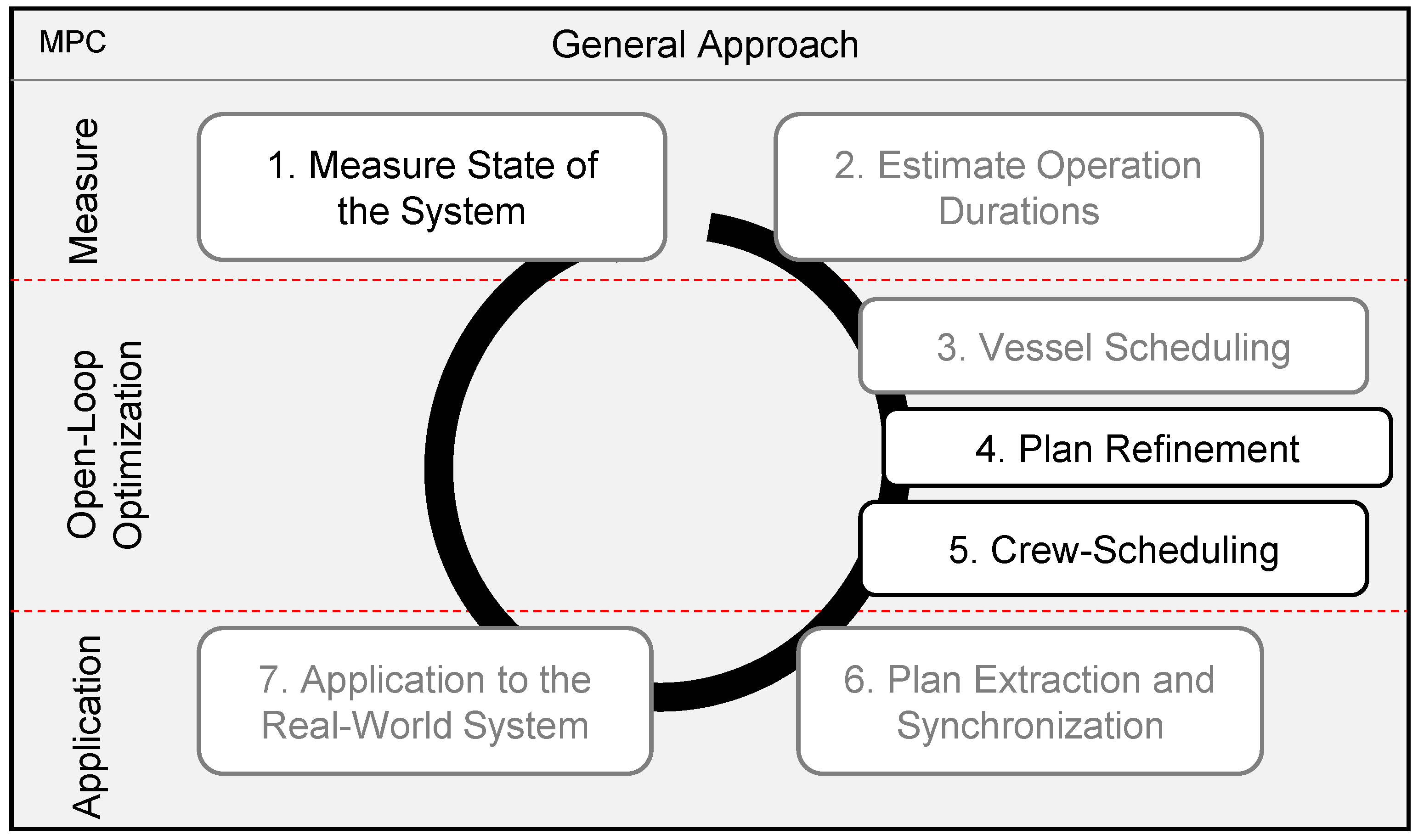
4. Workforce-Management Framework

As described before, the general concept proposed in this article follows a two-stage approach that first optimizes the operations performed by a vessel depending on current weather forecasts and measurements by using the approach described in Rippel et al. [10]. Afterward, it assigns personnel to these operations using a customized MILP model. The selected baseline approach applies incremental planning to reduce the influence of forecast uncertainties and defines monitoring and rescheduling policies for those cases that its predictions fail.
Figure 4 shows the extended approach, leaving unmodified steps in gray, while highlighting extended or new steps in black. Following the general Model Predictive Control scheme, the approach includes three phases with six steps that the approach applies incrementally as the installation progresses in the real-world system. The first phase measures the system state and updates the internal state representation, e.g., locations and loading states of vessels and the number of installed turbines. This section presents extensions of that system state x, required to enable an incremental crew scheduling. The second step uses weather forecasts to estimate the duration of each possible operation if a vessel would start it at a given instance during the planning horizon. The authors of the original approach propose two different ways to estimate these durations as a mixture of waiting and processing times: a Markov-Chain-based stochastic simulation and an estimation using a probabilistic sliding window approach. As the Markov-Chain approach delivers indeterministic results when applied to aggregate and basic operations (see step four for more details), this article proposes using the sliding window approach. The third step uses these estimated operation durations to optimize a long-term plan, spanning all included vessels. Following the Model Predictive Control scheme, this optimization generates a plan for P many planning horizons T denoted as the prediction horizon N = P · T . As the original model relies on so-called aggregate operations that, e.g., subsume all installation operations for a single turbine, including their associated waiting times, the fourth step refines these plans. Therefore, this step splits these aggregate operations into their contained basic operations and calculates their actual starting and end times by using the results of the sliding window estimation, also used to aggregate the operations. Step five uses this detailed list of operations to optimize the crew assignments for the long-term plan. Finally, steps six and seven extract the targeted short-term plan as control u that the approach forwards to the real-world system for execution. The approach defines its monitoring and rescheduling policy to trigger a new planning iteration if all operations in u have finished or if the real-world system diverges from u. The model aims to minimize offshore waiting times. Thus, it triggers a new instance if an operation finishes earlier than planned or takes longer and misses the next operation in u. Similarly, this article assumes that a new iteration will start if, e.g., personnel becomes unavailable during the plan execution due to accidents or sickness.

4.1. Model Design Based on the Requirements and General Assumptions

Particularly the crew scheduling model and its connected system state influence the fulfillment of the requirements stated earlier. Therefore, this subsection first revisits these requirements and describes how the proposed model aims to satisfy them before presenting the state x and the MILP model in more detail. In this context, this subsection also describes the general assumptions taken into account during the model design.
Working hours and rest periods: The proposed model uses the notion of rulesets ( r R ) that it assigns to each person or crew p P as r = R p to cope with different laws for parts of the overall crew. Each ruleset defines the maximum weekly ( W o r k l o a d r w e e k ) and daily ( W o r k l o a d r d a y ) workload, the length of daily rest periods ( R e s t r ), and the duration ( B r e a k r d u r ), and interval of short breaks ( B r e a k r i n t ) personnel need to take when working. The use of these rulesets allows differentiating, e.g., between port-side workers, project crews, or vessel crews that fall under different restrictions depending on the country’s laws.
Crew Roles and Qualification: In contrast to the articles found in the literature, the proposed model does not rely on a binary role model. Instead, it uses the notion of skills ( s S ). Therefore, it assigns each person a degree of experience for each noted skill as S p , s and a minimum required level of experience for each job as S j , s . This way of denoting capable personnel allows for a great deal of flexibility. Planners can define skills on a very rudimentary level, e.g., “We need persons that can install a blade with an experience of 1.5.”, or on way more detailed levels, e.g., “To install the blade, we need someone who can weld with an experience of 0.7 and someone who can operate the crane with an experience of 1.8”. The optimization model will then select crews that, combined, meet the minimum requirement of skills for each operation.
Availability and Worker Health: This requirement splits into two different aspects. First, the dynamic aspect of unavailability due to sickness or accidents. This proposed general approach already covers this aspect by its iterative planning and the described monitoring and rescheduling policy. Second, the requirement includes planned unavailabilities, e.g., due to vacation or on/off periods. The model covers this aspect by including a parameter ( P l a n n e d p , k ) in its state. It lists if a person (p) is already planned or unavailable for a given instance (k) within the prediction horizon. In addition to noting general unavailability, the model uses this parameter to block a rescheduling of personnel, e.g., if the plan for one vessel fails, while other vessels still have planned operations for the new prediction horizon left.
Types of Contract and Payment: Similar to the rulesets, which already cover most of the contractual characteristics, the model allows assigning costs to each person individually as C o s t p . By combining the rulesets and skills with the cost parameter, the model provides a versatile way to define different personnel, contract types, and associated costs. For example, by adding a person without limits on their workloads, all skills, and high costs, the model can easily represent the notion of additional agency personnel introduced by Leggate et al. [31].
Type of Assignment: The model’s design assigns crews to jobs. As described earlier, the fourth step of the general approach breaks down the provided plans into basic installation, loading, and vessel operations as specified in Table 1 to allow precise assignment with a high level of detail. Therefore, the model uses a set of jobs j J . For each job, the model denotes the jobs starting ( J o b j s t a r t ) and end time ( J o b j e n d ), its duration ( J o b j d u r ), and its indexed location ( L o c j j o b ), e.g., if it takes place at the port or a particular vessel. Similarly, it denotes the location of personnel ( L o c p p e r ). Using these locations, the model calculates a binary matching if a particular person or crew is present at the right location ( A t L o c p , j ) as part of the capability requirement.
Influence of Weather and Forecast-Uncertainty: Weather conditions strongly affect the overall planning problem and define when an operation can start safely. The proposed approach includes these dynamics in its general approach but not in the actual crew scheduling model. As described earlier, the general approach follows a predictive-reactive approach to first estimate the influence of weather conditions using forecasts, even including their uncertainty. Second, it employs viable monitoring and rescheduling policies to react if the predictions were wrong.
Nationality: As described earlier, this article focuses on the operative decision support and, thus, assumes that planners already took care of visa, traveling, and accommodation issues for planned crews or personnel. Thus, the model does not include the nationality of the crews explicitly.

4.2. System State for the Crew Scheduling (Model Parameters)

Besides the parameters already described in the last subsection, the system state contains additional (current) information, such as the current location of a person or crew, carryover information from the last iteration, or data on when a new week starts or ends.
Table 3 lists the state variable containing all parameters used in the optimization model. The model requires most of the current state information due to its incremental planning and the general approach’s reactive nature, which does not guarantee fixed time steps. For example, the model needs to track how many hours personnel has already worked during the current week and when it ends. Similarly, the model needs to know if personnel still needs to start or end a rest period on the current day and how many hours of pause they already had at the end of the last planning cycle.

4.3. Decision Variables and Cost Function

The proposed model uses a time-indexed formulation, where each index represents one hour. It uses six binary decision variables for its optimization. Four of these variables directly follow the definitions given in Rizvanolli and John [37] and Rizvanolli and Heise [38]. The model’s primary decision variable X p , j , k a t T i m e tracks if personnel p performs a specific job j at time k. Two additional variables track which person performs which job ( X p , j j o b ) and which person the model assigns to the current plan ( X p a s s i g n e d ). The fourth of these variables X p , j , k a c t i v e tracks if a person’s or crew’s state switches from active to inactive. The cost function later on uses this variable to avoid a quick switching between personnel and ensures that personnel remains active as long as possible. Finally, the model adds two additional decision variables, X p , k r e s t S and X p , k r e s t E , to track the start and end of resting periods. As can be seen from this definition, the optimizer primarily needs to decide on the assignment of personnel to jobs at a given time. The remaining variables directly depend on this decision and mainly simplify the definition of constraints.
Based on the cost function proposed in Rizvanolli and Heise [38], this model also minimizes the cost based on assigned personnel in X p a s s i g n e d . It also contains a term to minimize switching between personnel as the weighted, normalized sum of assignment changes. Equation (1) shows the applied cost function.
m i n p P X p a s s i g n e d · C o s t p + ϵ P · J · N · p P j J k N X p , j , k a c t i v e .

4.4. Constraints

The model uses several constraints to satisfy the requirements described above. In addition to the parameters described in the state, this article additionally introduces the notion of capable personnel, denoted as set P ¯ . The model deems personnel capable if they are at the right location ( A t L o c p , j = 1 ) and if they offer at least one skill required by the current job ( S p , s S j , s ). While the model calculates this set as needed, this article defines this set as given in Equation (2) for the sake of readability. In addition, constraints using this set enforce that their values become zero for unqualified personnel.
P ¯ = P | A t L o c p , j = 1 ( S p , s S j , s ) p P , j J , s S .
The remainder of this subsection presents the constraints and explains the reasoning behind them:
S j , s p P X p , j j o b · S p , s 0 j J , s S .
Constraint (3) ensures that the final plan satisfies all skill requirements imposed by the jobs.
t T X p , j , t a t T i m e = J o b j d u r · X p , j j o b j J , p P , T = J o b j s t a r t : J o b j e n d .
Constraint (4) ensures that if the model assigns personnel to a job, they perform the complete job. Additionally, the constraint ensures that the optimizer cannot assign more or less time to a job than defined by the duration parameter, even if the job allows starting and ending within a broader interval.
j J X p , j , k a t T i m e + P l a n n e d p , k 1 p P , k N .
Constraint (5) enforces that personnel only performs a single job at a time. Additionally, it prevents the model from scheduling already planned or unavailable personnel.
k N j J X p , j , k a t T i m e X p a s s i g n e d · N p P .
Constraint (6) denotes personnel assigned to a job at any time as assigned to the plan in general.
X p , j , t a c t i v e X p , j , t a t T i m e j J X p , j , t + 1 a t T i m e j J , p P ¯ , t J o b j s t a r t : J o b j e n d .
Constraint (7) tracks switches between active and inactive times for each person or crew. The constraint only applies to the set of capable personnel P ¯ .
j J t T X p , j , k a t T i m e 2 · R e s t R p · ( 1 X p , k r e s t S ) p P , k N , T = k : ( k 1 + R e s t R p )
j J t T X p , j , k a t T i m e 2 · R e s t R p · ( 1 X p , k r e s t E ) p P , k N , T = ( k + 1 R e s t R p ) : k .
Constraints (8) and (9) use a Big-M formulation to track the start and end of rest periods. The constraints force their respective variable to take the value of 0 if the period T contains any assignment for that person or crew. Both constraints only apply if period T fits into the planning problem, i.e., the model cannot denote the start of a rest period if the prediction horizon is too short to finish the period. Similarly, constraint (9) can only denote the end of a period, for instances larger or equal to the resting period.
Nevertheless, using the parameter P a u s e p l a s t , which contains the number of free hours personnel had at the end of the last iteration, an additional constraint allows the optimizer to use this time and schedule the end of a resting period that started in the last planning iteration. Therefore, the model calculates the remaining pause time as r e m P p .
R e s t R p P a u s e p l a s t + k 1 r e m P p X p , j , k a t T i m e p P , r e m P p k R e s t R p , + R e s t R p · 1 X p , k r e s t E r e m P p = R e s t R p P a u s e p l a s t .
Constraint (10) follows the same logic as the previous constraints but the model only applies it to the first time-instances k that are larger or equal to the remaining pause but smaller than the first viable instance for a regular resting period.
t t + 23 X p , t r e s t S 1 t t + 23 X p , t r e s t E 1 p P , t T = N | ( t + D a y S t a r t ) % 24 = 0
t t + 167 X p , t r e s t S 1 t t + 167 X p , t r e s t E 1 p P , t T = N | ( t + W e e k S t a r t ) % 168 = 0 .
Constraints (11) and (12) both contain two different constraints that require each day (11) and each week (12) to at least start and end one rest period per person or crew. The set T contains the instances where a new day or week starts within the prediction horizon. Its definition uses the modulo operator % that returns the rest of a division. Thus, for each instance starting a day or week, the optimizer requires that this instance and the following 23 instances (167 for weeks) include at least one pause start and pause end entry. A separate set of constraints focuses on the first interval between the first instance and D a y S t a r t . Instead of enforcing the start and end of a resting period, these additional constraints refer to the state parameters P a u s e p s t a r t and P a u s e p e n d to see if that person or crew still needs to start or finish its resting period for this day.
j J t t + 23 X p , j , k a t T i m e + P l a n n e d p , t W o r k l o a d R p d a y p P , t T = N | t + D a y S t a r t % 24 = 0
j J t t + 167 X p , j , k a t T i m e + P l a n n e d p , t W o r k l o a d R p w e e k p P , t T = N | t + W e e k S t a r t % 168 = 0 .
Constraints (13) and (14) use the same day and week indices T to limit the maximum workload per person or crew for each day and week. Similar to the last constraints, the first periods for the day and week additionally add the state parameters W o r k e d p d a y and W o r k e d p w e e k to allow for the model’s incremental planning.
j J k k 1 + B r e a k R p i n t X p , j , k a t T i m e B r e a k R p i n t B r e a k R p d u r p P , k N .
Finally, constraint (15) requires each instance k that the following time interval, defined by the pause interval, contains a break according to the current person’s or crew’s ruleset. Therefore, it limits the maximum number of assigned hours for this interval.

5. Experiments and Results

The experiments conducted for this article use an implementation of the framework and the proposed model in MATLAB 2018b using MATLAB’s problem-based formulation to specify the optimization problems. Furthermore, the experiments use Gurobi 9.1 to solve the optimization. All experiments were conducted on a standard desktop computer, using an AMD Ryzen 9 3900X 12-Core Processor with 32 GB of memory.

5.1. Scenario Description

The experiments apply the same installation scenario introduced by Beinke et al. [19] and used the original publication of the online approach for the operation scheduling. The scenario represents a real-world use-case with an installation site in Germany’s Northern Sea and a base port in Eehmshaven, Netherlands. In addition to the times and restrictions given in Table 1, traveling between the base port and the installation site takes four hours. The scenario applies one and two installation vessels with a capacity of four to install 25 turbines. It uses a planning horizon of two weeks and two planning periods.
As the original scenario depicts a German installation project, this article chooses German Laws to parameterize the crew scheduling. Accordingly, it applies three different rule sets for port-side workers, the vessel crew, and the installation or project crew. Moreover, the scenario adds an agency crew to each location to accommodate unexpected demand spikes. While the model’s design allows to schedule individuals, this experiment simplifies the staffing to full crews. For example, a project crew consists of a fixed team of people who have the necessary experience to perform any installation task. Accordingly, the scenario uses three skills (Port, Vessel, and Installation), each job requires one of them, and each crew offers one of these skills.
The state of the art shows that all articles in the literature assume that planners assign sufficient personnel to cover work for 24 h a day, seven days a week. Consequently, the scenario takes the same assumption. Generally, the weekly workload imposes a stronger restriction and results in the use of five port crews (168 h/40 h = 4.2 Crews), three vessel crews (168 h/72 h = 2.3 Crews), and four installation crews (168 h/48 h = 3.5 Crews). Table 4 summarizes the main parameters for this scenario.
As the crew scheduling mainly depends on the provided plans for vessels, the experiments cover different starting dates for the installation. Therefore, this article selects the first of each month between April and September 2000 to simulate the real-world process, using historical weather recordings. These months show distinct characteristics considering their conditions, i.e., August shows close to perfect weather conditions for installation projects. September contains several long bad-weather windows. The rest provide a good mix of both.
In addition to the experiments described above, the experiments also include an extended scenario. Besides following the same settings and parameterizations, the extended scenario splits the installation crew into additional personnel with dedicated skills. Moreover, each operation requires several of the provided skills, effectively forming the required crew. Table 5 shows the required skills per operation and the minimum amount of personnel to provide this skill. Besides those occupations shown in the table, the scenario also includes mechatronics, who each provide the skills mechanic, electrician, and welder. Apart from the crane operator, all crew members with these new roles use the restrictions for project crews described above. Nevertheless, crane operators usually belong to the vessel’s crew and use the appropriate ruleset.
Similar to the base scenario described above, this extended scenario assumes that each required role needs to be staffed with enough personnel to guarantee 24 h availability. Therefore, the scenario assumes three shifts per role and multiplies that with the maximum number of persons required for each operation. For example, the scenario includes six mechanics ( 2 × 3 ) but only three welders ( 1 × 3 ). In total, the scenario includes 43 personnel available to the optimizer.

5.2. Experimental Results

The experiments first provide a proof of concept for the proposed model and approach and show their viability and adherence to the imposed requirements. Moreover, the results shortly discuss the computational characteristics of this approach. Finally, this article compares incremental plans with optimal non-incremental plans to gain an impression of the planning quality. It has to be noted that such non-incremental plans would not be possible to obtain in real-world situations due to uncertainties associated with weather forecasts.
The results show that the model includes pauses and rest periods in all twelve simulated scenarios as required by law. Moreover, it consistently ensures adherence to the maximum daily and weekly workload for all crews. In general, the results demonstrate that fully staffing each vessel 24/7 would have been unnecessary in all cases.

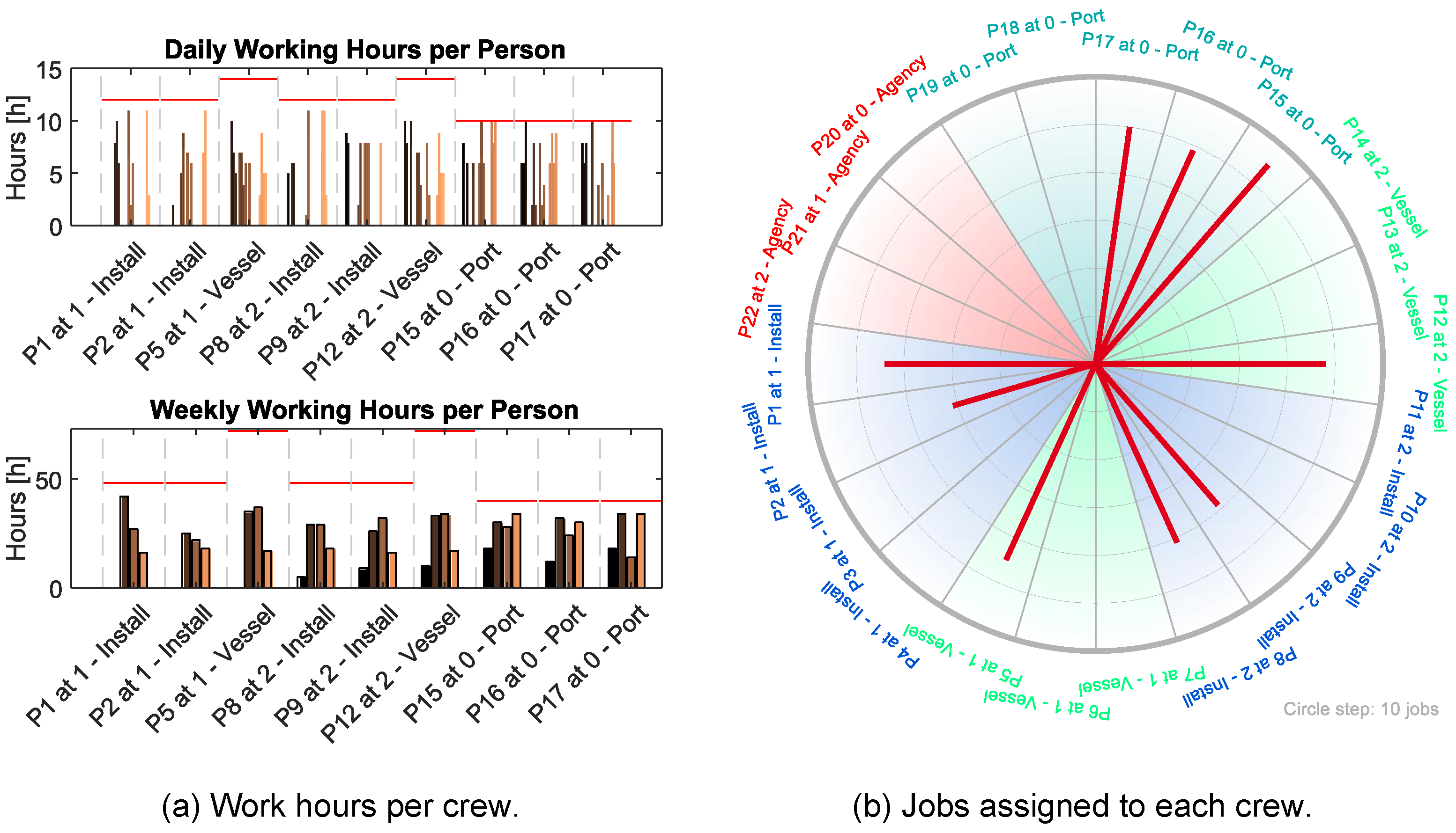
5.2.1. Base Scenario

Table 6 summarizes the averaged results across all simulation runs for the base scenario using three crew types.
The results show a drastic decrease in required crews. Comparing the incremental approach with full staffing, the model only requires 63% of port crews, 33% of the vessel crews, and 53% of available project crews per vessel, effectively reducing the overall required staff by about 49.7%. Compared to non-incremental optimal plans, the statistics given in Table 6 do not change between both types, apart from an increasing computational time for the non-incremental plans.
Figure 5 exemplary shows one of these scenarios in more detail. The scenario applies two installation vessels and selects the starting date as 1 July 2000. Figure 5a shows the distribution of working hours for each assigned crew per day and week for this scenario. The figure demonstrates that the model satisfies all restrictions. Moreover, the vessel crew shows a comparably low utilization if only considering installation-related tasks for this crew. Finally, Figure 5b shows the number of assigned jobs per crew. The figure shows that the crew scheduling did not assign any agency crews and avoided other available crews, as described above.

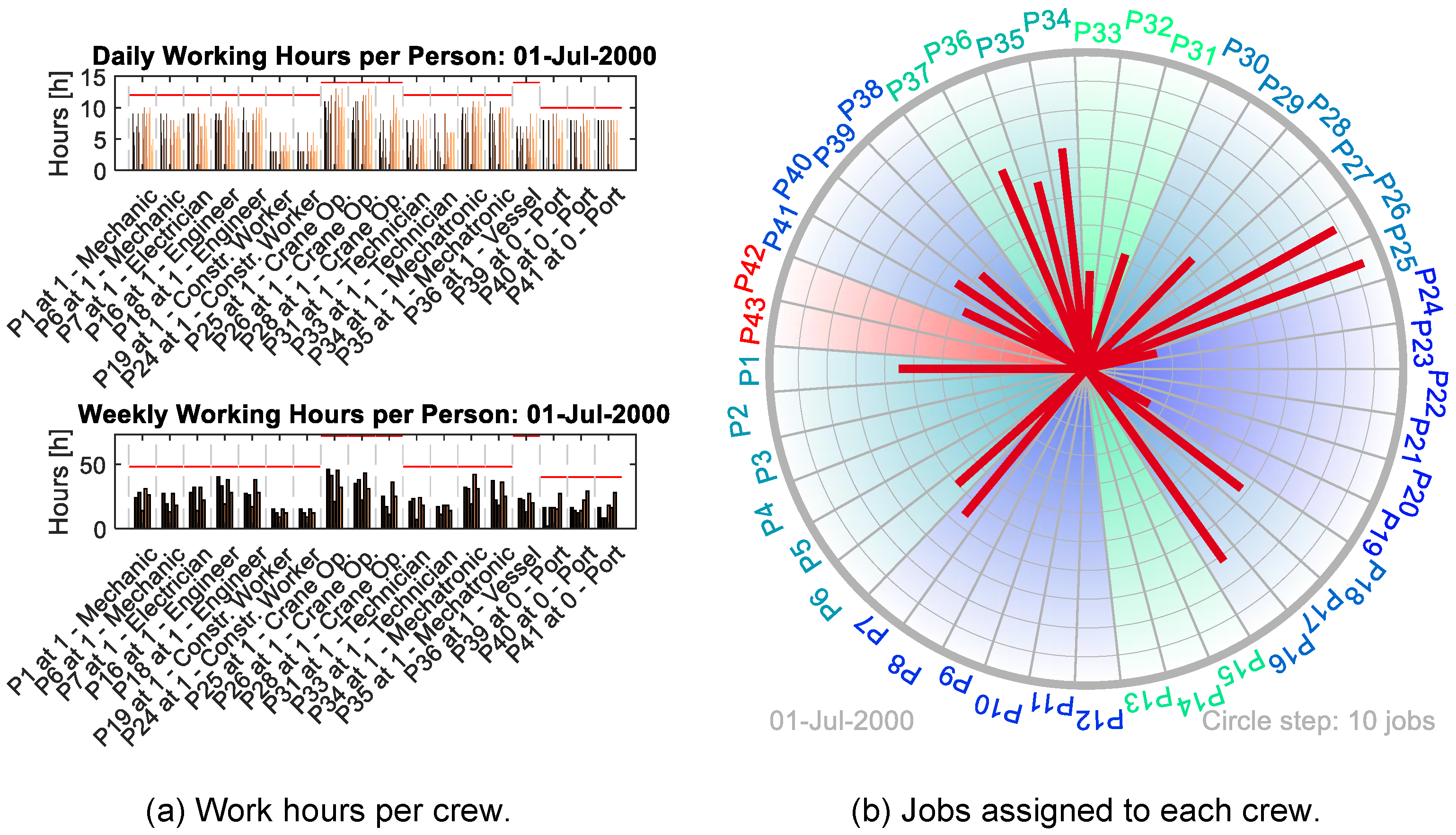
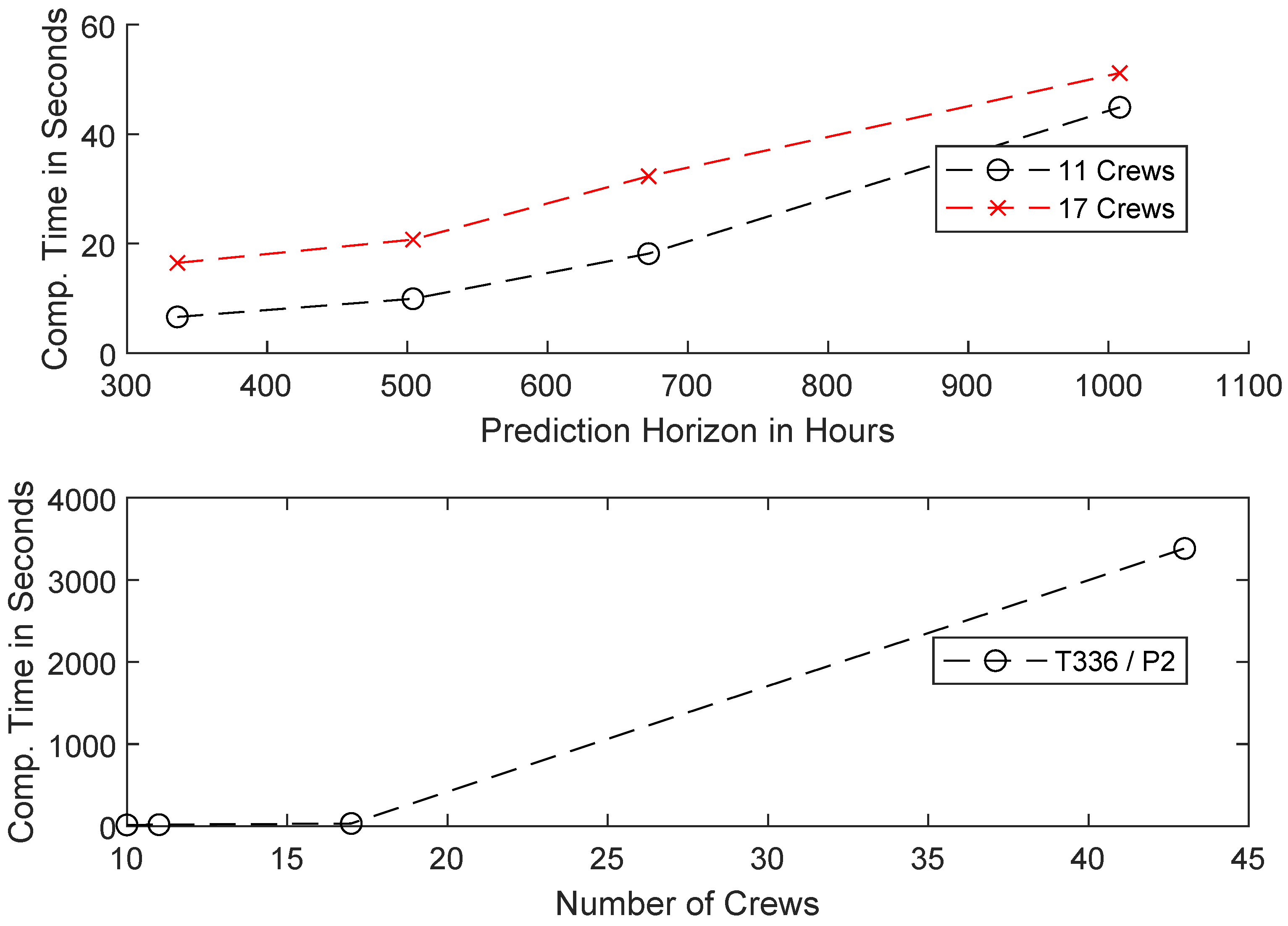
5.2.2. Extended Scenario and Computational Times

The extended scenario aims to demonstrate the model’s ability to handle higher levels of detail than covered in the base scenario. Similar to the base scenario, the results show that the model guarantees adherence to working hour limits and to pause and rest times for all personnel. Moreover, the model only requires 18 of the available 43 personnel (41.9%) and tries to split the workload evenly between similar personnel. Figure 6 exemplary shows the results for July 2000.
Besides showcasing the model’s general ability to handle different levels of detail flexibly, this scenario allows a more detailed investigation of the model’s runtime behavior considering the number of crews. In general, scheduling problems belong to the class of NP-hard, in most cases NP-complete problems. As the proposed model employs a time-indexed formulation, the complexity mainly depends on the number of personnel and the planning horizon. To allow a closer examination of these influences, Figure 7 depicts the computational time for selected experiments. The experiment covers additional simulation runs using the base scenario and varying prediction horizons, using a sampling width of one and two weeks and two and three prediction periods each, to establish a baseline for the influence of the planning horizon.
Figure 7a shows a slight but still exponential increase in the required (average) computational time for an increasing prediction horizon. While the experiments using two vessels show a more linear increase, the single vessel experiments show an exponential shape. Nevertheless, the times increase from 6.6 and 16.5 s to 44.9 and 51.2 s per planning iteration when increasing the prediction horizon from two weeks (168 h × 2) to six weeks (336 h × 3). The uncertainties involved with weather forecasts render longer prediction horizons unlikely in realistic applications.
Figure 7b shows the computational times for four different crew sizes given the same prediction horizon of four weeks (336 h × 2) used in most of the experiments. The graph shows a drastic increase between 17 crews (two vessels, base scenario) and 43 crews (extended scenario). For less than 17 crews, the figure shows low computational times, so that merely no difference can be seen in the figure. Nevertheless, these small crew sizes show a close to linear increase from 14.8 s for ten crews, over 18.2 s for 11 crews, to 32.3 s for 17 crews. Nevertheless, the drastic increase to 3382.9 s (approximately 58 min) for 43 crews clearly demonstrates the exponential increase expected from NP-hard scheduling problems.

6. Conclusions and Outlook

This article presents a framework for crew scheduling in offshore constructions. Therefore, it first presents a literature analysis to define legal and domain-specific requirements for the crew scheduling. Afterward, it presents a new crew scheduling formulation by reusing and extending an existing formulation from the literature. The article proposes to combine this model with an incremental scheduling approach, which derives weather-dependent vessel schedules, to handle dynamics in the application domain. Finally, the article evaluates the proposed approach using twelve scenarios that closely follow a real-world use case. It also includes further experiments to demonstrate the model’s ability to handle larger problem instances and evaluate its runtime behavior.
In conclusion, the results show that the model provides law-compliant crew schedules when used incrementally and non-incrementally. Compared to completely staffing vessels or the port, applying the proposed approach can save approximately half the crews. Comparing incremental and non-incremental planning shows no difference considering the number of applied crews. Finally, the selected cost function shows an interesting property over other cost functions, which were evaluated but not presented in this article. While variants based on hourly costs of personnel tend to fully utilize personnel with lower costs and avoid higher cost personnel, the proposed cost function distributes work evenly between personnel planned for a trip. As companies usually pay offshore personnel per project or month, an even distribution seems desirable. The even distribution, visible in Figure 5, results from the combination of cost terms, i.e., personnel inflicts the same costs no matter if they perform one or fifty jobs over the prediction horizon. The additional term that keeps personnel active as long as possible results in a pretty even distribution of personnel with similar contracts and qualifications. The results considering the model’s runtime behavior show that the model solves the imposed scheduling problem in a reasonable time. Coarsely defined problems, only focusing on predetermined crews, show a runtime of less than a minute. Extended definitions that focus on single persons showed a runtime of approximately one hour when using a realistic planning horizon of four weeks. As offshore installations usually have operation times in the range of several hours, it can be expected that high detailed plans with reasonable numbers of personnel can be solved fast enough to apply the proposed model in real-time. In addition, further developments of heuristics or tweaks for the optimizer settings can speed up the computation. The current experiments used GUROBI’s exact branch-and-bound solution method with its default settings. Examining the optimization logs for the extended scenario showed that GUROBI determined the final solution in all cases in less than 20 min at a gap between the theoretically best possible solution and the final encumberment of less than 5%. The rest of the time, it used to prove that this actually was the optimal solution. In conclusion, allowing for a gap of 5% would have yielded the optimal solution in under 20 min for all extended scenarios. Another way to reduce the computational time would be to reduce the number of available personnel. The experiments always provided enough personnel for full availability. All experiments show that this assumption leads to a drastic overestimation (approximately 50%) and, thus, results in excess computational requirements.
Among others, future work will focus on further developing the model and the embedding framework. On the one hand, it will investigate recovery-type formulations to reduce the impact of rescheduling on the crew assignments. Changes to the monitoring and rescheduling policy or the model itself might reduce the influence of uncontrollable dynamics, such as accidents. On the other hand, future work will investigate achieving a higher degree of integration between the two scheduling models. Currently, the operation schedule takes priority and remains unchanged even if slight changes might reduce the need for additional crews or persons.

Author Contributions

Conceptualization, F.A.F. and D.R.; methodology, D.R.; software, D.R.; validation, D.R. and F.A.F.; investigation, F.A.F.; resources, M.F.; writing—original draft preparation, D.R. and F.A.F.; writing—review and editing, M.L. and M.F.; visualization, D.R.; supervision, M.L. and M.F.; project administration, M.L.; funding acquisition, D.R. and M.L. All authors have read and agreed to the published version of the manuscript.

Funding

The authors gratefully acknowledge the financial support by the German Research Foundation (DFG) for the research project “OffshorePlan”, grant number (LU 2049/1-1|SZ 51/33-1). The APC was funded by the German “Staats- und Universätsbibilothek Bremen”.

Institutional Review Board Statement

Not applicable.

Informed Consent Statement

Not applicable.

Data Availability Statement

This article’s evaluation uses commercially available data sets of historical wind and wave records from Germany’s North Sea between 1956 and 2012.

Conflicts of Interest

The authors declare no conflict of interest.

References

  1. REN21. Renewables 2021 Global Status Report. 2021. Available online: https://www.ren21.net/reports/global-status-report/ (accessed on 14 September 2021).
  2. BVGassociates. Guide to an Offshore Wind Farm. 2019. Available online: https://bvgassociates.com/publications/ (accessed on 14 September 2021).
  3. Beinke, T.; Ait Alla, A.; Oelker, S.; Freitag, M. Demand for Special Vessels for the Decommissioning of Offshore Wind Turbines in the German North Sea—A Simulation Study. In Proceedings of the 30th International Ocean and Polar Engineering Conference (ISOPE), Virtual, 1–16 October 2020; Chung, J.S., Akselsen, O.M., Jin, H., Kawai, H., Lee, Y., Matskevitch, D., Eds.; ISOPE: Cupertino, CA, USA, 2020; pp. 480–484. [Google Scholar]
  4. Breton, S.; Moe, G. Status, Plans and Technologies for Offshore Wind Turbines in Europe and North America. Renew. Energy 2009, 34, 646–654. [Google Scholar] [CrossRef]
  5. Dewan, A.; Asgarpour, M.; Savenije, R. Commercial Proof of Innovative Offshore Wind Installation Concepts Using Ecn Install Tool; ECN: Petten, The Netherlands, 2015. [Google Scholar]
  6. Muhabie, Y.T.; Rigo, P.; Cepeda, M.; D’Agosto, M.A. A Discrete-event Simulation Approach to Evaluate the Effect of Stochastic Parameters on Offshore Wind Farms Assembly Strategies. Ocean Eng. 2018, 149, 279–290. [Google Scholar] [CrossRef]
  7. Ait Alla, A.; Oelker, S.; Lewandowski, M.; Freitag, M.; Thoben, K.D. A Study of New Installation Concepts of Offshore Wind Farms by Means of Simulation Model. In Proceedings of the Twenty-seventh International Ocean and Polar Engineering Conference (ISOPE), San Francisco, CA, USA, 25–30 June 2017; Chung, J.S., Triantafyllou, M.S., Langen, I., Eds.; ISOPE: Cupertino, CA, USA, 2017; pp. 607–612. [Google Scholar]
  8. Vis, I.F.; Ursavas, E. Assessment Approaches to Logistics for Offshore Wind Energy Installation. Sustain. Energy Technol. Assess. 2016, 14, 80–91. [Google Scholar] [CrossRef] [Green Version]
  9. Oelker, S.; Lewandowski, M.; Ait Alla, A.; Ohlendorf, J.H.; Haselsteiner, A.F. Logistikszenarien Für Die Errichtung Von Offshore-windparks—Herausforderungen Der Wirtschaftlichkeitsbetrachtung Neuer Logistikkonzepte. Ind. 4.0 Manag. 2017, 33, 24–28. [Google Scholar]
  10. Rippel, D.; Jathe, N.; Lütjen, M.; Freitag, M. Evaluation of Loading Bay Restrictions for the Installation of Offshore Wind Farms Using a Combination of Mixed-integer Linear Programming and Model Predictive Control. Appl. Sci. 2019, 9, 5030. [Google Scholar] [CrossRef] [Green Version]
  11. Rippel, D.; Jathe, N.; Becker, M.; Lütjen, M.; Szczerbicka, H.; Freitag, M. A Review on the Planning Problem for the Installation of Offshore Wind Farms. IFAC-PapersOnLine 2019, 52, 1337–1342. [Google Scholar] [CrossRef]
  12. Scholz-Reiter, B.; Karimi, H.R.; Lütjen, M.; Heger, J.; Schweizer, A. Towards a Heuristic for Scheduling Offshore Installation Processes. In Proceedings of the 24th International Congress on Condition Monitoringand and Diagnostics Engineering Management. Advances in Industrial Integrated Asset Management, Birmingham, UK, 30 May–1 June 2011; Maneesh, S., Rao, R., Liyanage, J.P., Eds.; COMADEM International: Birmingham, UK, 2011; pp. 999–1008. [Google Scholar]
  13. Ait Alla, A.; Quandt, M.; Lütjen, M. Simulation-based Aggregate Installation Planning of Offshore Wind Farms. Int. J. Energy 2013, 7, 23–30. [Google Scholar]
  14. Kerkhove, L.P.; Vanhoucke, M. Optimised Scheduling for Weather Sensitive Offshore Construction Projects. Omega 2017, 66, 58–78. [Google Scholar] [CrossRef]
  15. Ursavas, E. A Benders Decomposition Approach for Solving the Offshore Wind Farm Installation Planning at the North Sea. Eur. J. Oper. Res. 2017, 258, 703–714. [Google Scholar] [CrossRef]
  16. Barlow, E.; Tezcaner Öztürk, D.; Revie, M.; Akartunalı, K.; Day, A.H.; Boulougouris, E. A Mixed-method Optimisation and Simulation Framework for Supporting Logistical Decisions during Offshore Wind Farm Installations. Eur. J. Oper. Res. 2018, 264, 894–906. [Google Scholar] [CrossRef] [Green Version]
  17. Irawan, C.A.; Wall, G.; Jones, D. An Optimisation Model for Scheduling the Decommissioning of an Offshore Wind Farm. OR Spectr. 2019, 41, 513–548. [Google Scholar] [CrossRef]
  18. Lange, K.; Rinne, A.; Haasis, H.D. Planning Maritime Logistics Concepts for Offshore Wind Farms: A Newly Developed Decision Support System. Lect. Notes Comput. Sci. Comput. Logist. 2012, 7555, 142–158. [Google Scholar]
  19. Beinke, T.; Ait Alla, A.; Freitag, M. Resource Sharing in the Logistics of the Offshore Wind Farm Installation Process Based on a Simulation Study. Int. J. E-Navig. Marit. Econ. 2017, 7, 42–54. [Google Scholar] [CrossRef]
  20. Quandt, M.; Beinke, T.; Ait Alla, A.; Freitag, M. Simulation Based Investigation of the Impact of Information Sharing on the Offshore Wind Farm Installation Process. J. Renew. Energy 2017, 2017, 11. [Google Scholar] [CrossRef] [Green Version]
  21. Cheng, M.Y.; Wu, Y.F.; Wu, Y.W.; Ndure, S. Fuzzy Bayesian schedule risk network for offshore wind turbine installation. Ocean Eng. 2019, 188, 106238. [Google Scholar] [CrossRef]
  22. Peng, S.; Szczerbicka, H.; Becker, M. Modeling and Simulation of Offshore Wind Farm Installation with Multi-Leveled CGSPN. In Proceedings of the 30th International Ocean and Polar Engineering Conference (ISOPE), Virtual, 11–16 October 2020; Chung, J.S., Akselsen, O.M., Jin, H., Kawai, H., Lee, Y., Matskevitch, D., Eds.; ISOPE: Cupertino, CA, USA, 2020; pp. 472–479. [Google Scholar]
  23. Moher, D.; Liberati, A.; Tetzlaff, J.; Altman, D.G. Preferred reporting items for systematic reviews and meta-analyses: The PRISMA statement. PLoS Med. 2009, 6, e1000097. [Google Scholar] [CrossRef] [Green Version]
  24. van den Bergh, J.; Beliën, J.; de Bruecker, P.; Demeulemeester, E.; de Boeck, L. Personnel scheduling: A literature review. Eur. J. Oper. Res. 2013, 226, 367–385. [Google Scholar] [CrossRef]
  25. Gopalakrishnan, B.; Johnson, E.L. Airline Crew Scheduling: State-of-the-Art. Ann. Oper. Res. 2005, 140, 305–337. [Google Scholar] [CrossRef]
  26. John, O.; Gailus, S.; Rizvanolli, A.; Rauer, R. An Integrated Decision Support Tool for Hours of Work and Rest Compliance Optimization during Ship Operations. In Proceedings of the 13th International Conference on Computer and IT Applications in the Maritime Industries, COMPIT’14, Redworth, UK, 12–14 May 2014; Bertram, V., Ed.; Schriftenreihe Schiffbau, Technology University Verlag Schriftenreihe Schiffbau: Hamburg, Germany, 2014; pp. 245–257. [Google Scholar]
  27. Bundesamt für Justiz und Verbraucherschutz. Verordnung über die Arbeitszeit bei Offshore-Tätigkeiten; Bundesamt für Justiz and Verbraucherschutz: Berlin, Germany, 2013. [Google Scholar]
  28. Bundesamt für Justiz and Verbraucherschutz. Seearbeitsgesetz (SeeArbG); Bundesamt für Justiz and Verbraucherschutz: Berlin, Germany, 2021. [Google Scholar]
  29. Colli, N.; Mache, S.; Harth, V.; Mette, J. Physische und psychische Gesundheit von Offshore-Beschäftigten. Zentralblatt für Arbeitsmedizin Arbeitsschutz und Ergon 2017, 67, 176–178. [Google Scholar] [CrossRef]
  30. Hammer, G.; Röhrig, R. Qualification Requirement Analysis Offshore Wind Energy Industry. Tech. Rep. 2005. Available online: http://pcoe.nl/@api/deki/files/1919/=15final_report_qrs.pdf (accessed on 21 October 2021).
  31. Leggate, A.; Sucu, S.; Akartunalı, K.; van der Meer, R. Modelling crew scheduling in offshore supply vessels. J. Oper. Res. Soc. 2018, 69, 959–970. [Google Scholar] [CrossRef]
  32. Sucu, S. Solving Crew Scheduling Problem in Offshore Supply Vessels: Heuristics and Decomposition Methods. Ph.D. Thesis, University of Strathclyde, Glasgow, Scotland, 2017. [Google Scholar]
  33. Giachetti, R.E.; Damodaran, P.; Mestry, S.; Prada, C. Optimization-based decision support system for crew scheduling in the cruise industry. Comput. Ind. Eng. 2013, 64, 500–510. [Google Scholar] [CrossRef] [Green Version]
  34. Damodaran, P.; Mestry, S.; Zuniga, M.; Perez, J.; Brearley, R.; Arteta, B. A mathematical model for scheduling shipboard crew in cruise lines. In Proceedings of the IIE Annual Conference Expo 2010 Proceedings, Boston, MA, USA, 23–25 June 2010. [Google Scholar]
  35. Sereno, V.M.; Reinhardt, L.B.; Guericke, S. Exact Methods and Heuristics for the Liner Shipping Crew Scheduling Problem. In Computational Logistics; Cerulli, R., Raiconi, A., Voß, S., Eds.; Lecture Notes in Computer Science; Springer International Publishing: Cham, Switzerland, 2018; Volume 11184, pp. 363–378. [Google Scholar] [CrossRef]
  36. Leggate, A. A Vessel Crew Scheduling Problem: Formulations and Solution Methods. Ph.D. Thesis, University of Strathclyde, Glasgow, Scotland, 2016. [Google Scholar]
  37. Rizvanolli, A.; John, O. Ein gemischt-ganzzahliges lineares Optimierungs- modell zur Ermittlung des minimal notwendigen Bedarfes an Seefahrern zur Besetzung eines Schiffes. In Entscheidungsunterstützung in Theorie und Praxis; Spengler, T., Fichtner, W., Geiger, M.J., Rommelfanger, H., Metzger, O., Eds.; Springer Fachmedien Wiesbaden: Wiesbaden, Germany, 2017; pp. 87–107. [Google Scholar] [CrossRef]
  38. Rizvanolli, A.; Heise, C.G. Efficient Ship Crew Scheduling Complying with Resting Hours Regulations. In Operations Research Proceedings 2016; Fink, A., Fügenschuh, A., Geiger, M.J., Eds.; Operations Research Proceedings; Springer International Publishing: Cham, Switzerland, 2018; pp. 535–541. [Google Scholar] [CrossRef]
Figure 1. Conventional installation concept [10].
Energies 14 06963 g001
Figure 2. Crew Scheduling Procedure extended from Reference [26].
Energies 14 06963 g002
Figure 3. Results after evaluating existing models against the requirements.
Energies 14 06963 g003
Figure 4. General Approach. Extended from Reference [10].
Energies 14 06963 g004
Figure 5. Exemplary results for the scenario July 2000 with two vessels.
Energies 14 06963 g005
Figure 6. Exemplary results for the scenario July 2000 with one vessel and extended crew.
Energies 14 06963 g006
Figure 7. Computational time depending on the planning horizon (top) and the number of personnel (bottom).
Energies 14 06963 g007
Table 1. Operations, limits, and durations—extended from Reference [10].
OperationBase-DurationMax. WindMax. WaveResponsible
[h][m/s][m]Crew
Load Tower312 15 1Port Crew
Load Nacelle212 15 1Port Crew
Load Hub112 15 1Port Crew
Load Blade212 15 1Port Crew
Traveling4212.5Vessel Crew
(Re-)Positioning1142.0Vessel Crew
Jack-up/-down2141.8Vessel Crew
Install Tower3122.5 2Project Crew
Install Nacelle3122.5 2Project Crew
Install Hub2122.5 2Project Crew
Install Blade2102.5 2Project Crew
1 Mostly omitted by using loading bridges. 2 High values due to jack-up stabilizing the vessel.
Table 2. Articles proposing models with similar problems by domain and year of publication.
PublicationObjectiveDomainHorizon
Damodaran et al. (2010) [34]Min. CostCruise-Lanes1 Year
Giachetti et al. (2013) [33]Min. Trip CostCruise-Lanes240 Days
John et al. (2014) [26]Min. CostShipping LinesOne Trip
Sereno et al. (2018) [35]Min. Trip CostShipping Lines1 Year
Leggate (2016) [36]Min. CostOffshore Supply3+ Months
Sucu (2017) [32]Min. CostOffshore Supply3+ Months
Leggate et al. (2018) [31]Min. Cost andOffshore Supply3+ Months
Min. Num Changes
Rizvanolli and John (2017) [37]Min. CrewContainer Transp.One Trip
Rizvanolli and Heise (2018) [38]Min. CrewContainer Transp.One Trip
Table 3. Complete state model.
ParameterSymbolUnitDomain
Sets and Indices
Prediction Horizon N = P · T k N Hours N +
Set of Persons/Crews p P Persons-
Set of Jobs j J Jobs-
Set of Locations L Locations-
Set of Skills s S Skills-
Rule Sets r R Rulesets-
Job Information
Job Start Instance J o b j s t a r t Hour N +
Job End Instance J o b j e n d Hour N +
Job Duration J o b j d u r Hours N +
Location of Job L o c j j o b Location N +
Assignment of Req. Skills to Jobs S j , s Experience R 0 +
Personnel Information
Assignment of Ruleset to Persons R p Index N +
Assignment of Skills to Persons S p , s Experience R 0 +
Cost per Person C o s t p Currency R 0 +
Ruleset Information
Maximum Daily Workload W o r k l o a d r d a y Hours N +
Maximum Weekly Workload W o r k l o a d r w e e k Hours N +
Rest Period R e s t r Hours N +
Length of Breaks B r e a k r d u r Hours N +
Break Interval (One Break each) B r e a k r i n t Hours N +
Current State Information
Availability of Person P l a n n e d p , k UnavailableBinary
Location of Personnel L o c p p e r Location N +
Presence of Person at Job Location A t L o c p , j At LocationBinary
Index of Next Week W e e k S t a r t Hours N +
Index of Next Day D a y S t a r t Hours N +
Needs to Start Rest Today P a u s e p s t a r t RequiresBinary
Needs to End Rest Today P a u s e p e n d RequiresBinary
Hours Worked Today W o r k e d p d a y Hours N +
Hours Worked This Week W o r k e d p w e e k Hours N +
Free Time at End of the Last Iteration P a u s e p l a s t Hours N +
Table 4. Parameters for the crew scheduling.
ParameterPort CrewVessel CrewProject CrewAgency
Maximum Daily Workload14121024
Maximum Weekly Workload724840168
Rest Period611110
Length of Breaks1110
Break Interval101080
Number per Location5341
Table 5. Required skills per operation in the extended scenario.
Inst. TowerInst. NacelleInst. BladeInst. Hub
Mechanic2122
Electrician1212
Welder1000
Engineer1111
Construction Worker2000
Crane Operator1122
Technician1101
Table 6. Average results across all twelve simulation runs for the base scenario.
Result
Key-Performance IndicatorAllOne VesselTwo Vessels
Average Number of Jobs Scheduled390.92
Average Project Duration771 h1007 h535 h
Average Number of Planning Iterations2.753.172.33
Total Number of Plan Interruptions10.04.006.00
Average Optimization Time per Iteration25.25 s18.17 s32.32 s
Average Port Crews Required3.173.003.33
Average Vessel Crews Required1.501.002.00
Average Project Crews Required3.172.174.17
Publisher’s Note: MDPI stays neutral with regard to jurisdictional claims in published maps and institutional affiliations.

