1. Introduction
The market related to the building air conditioning systems employing ground coupled heat pump (GCHP) involves about one million installations in Europe. As reported by the International Energy Agency (IEA) [
1], Sweden and Germany are the two main European markets, with 20,000 up to 30,000 new installations every year in each country. More than half of GCHP in the world are installed in the United States. According to [
1], electric heat pumps could supply more than 90% of air and water heating with lower CO
2 emissions than the condensing gas boiler technology (92–95% efficiency), even when the primary carbon intensity of electricity consumption is taken into account. GCHP applications are composed of a heat pump coupled with the ground through multiple vertical or horizontal ground heat exchangers constituting a closed-loop system. Typically, vertical borehole heat exchangers (BHEs) are the most frequently adopted solution.
For the correct sizing of these closed-loop systems and their energy and economic sustainability, it is important to know the ground thermal parameters. One of the more simple to use and in any case reliable methods for sizing a BHE field is the Ashrae method improved with the Tp8 approach [
2,
3]. However, also in this case, the thermal conductivity of both the ground and the backfilling material (also known as grout) must be estimated (or similarly the couple ground thermal conductivity and BHE thermal resistance).
Ground thermal conductivity and BHE thermal resistance are typically evaluated through a measurement procedure called Thermal Response Test (TRT). The TRT was first proposed by Mogensen [
4] and it is based on the Infinite Line Source model (ILS, Carslaw and Jaeger [
5], Ingersoll et al. [
6]). Pure heat conduction in an infinite medium, constant heat transfer rate in time and space from a linear source, and uniform ground thermal properties are the main assumptions of the ILS model.
The TRT experiment is based on constantly heating (or cooling) the carrier fluid flowing through a pilot BHE while continuously measuring the inlet and outlet fluid temperatures. The effective ground thermal conductivity together with the effective borehole thermal resistance can be estimated from the slope and the intercept of the average fluid temperature profile.
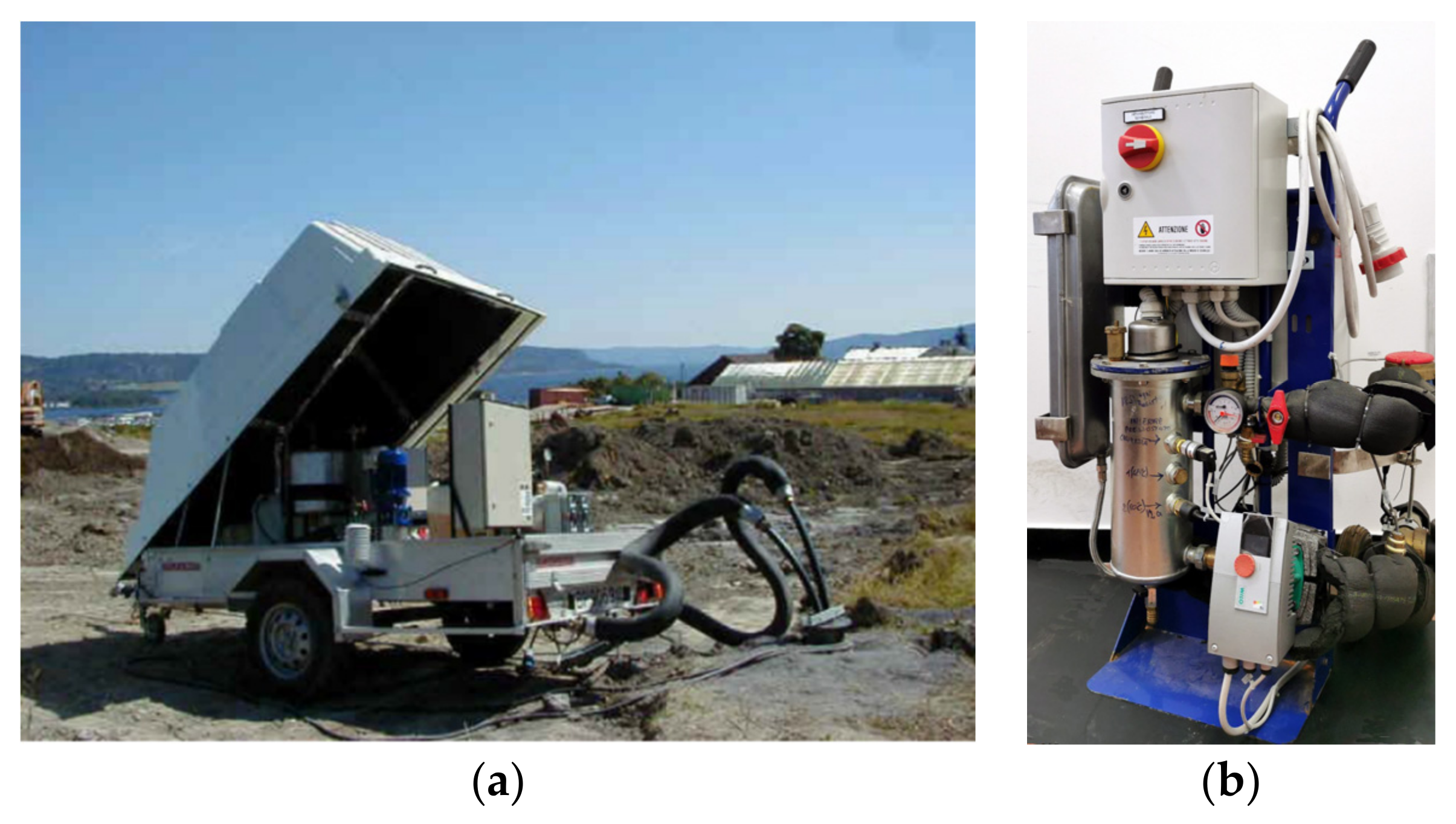
Dedicated experimental equipment, the so-called TRT machines (shown in
Figure 1), are used to perform the measurement campaigns. The first moveable measurement devices were introduced by Eklöf and Gehlin [
7], Austin [
8] and Gehlin [
9]. Unfortunately, these machines have a particularly high realisation cost (EUR 20,000–60,000 from 2019 estimates).
A diffused literature about TRT and comprehensive analysis of the related methods are available [
10,
11]. A general analysis of the various TRT types, including standard TRT, pulsated TRT (Fossa et al. [
12]) and Distributed Thermal Response Test (DTRT) with fibre optics using the Raman effect is discussed by Acuña et al. [
13]; the theoretical basis of the method is, for example, reported by Franco and Conti [
14].
Among conventional 1D radial models that can be used for TRT analysis, a cylindrical-source model neglecting the thermal storage of the fluid (and the grout if present) within the borehole has been applied to boreholes by Ingersoll et al. [
6,
15] and Deerman and Kavanaugh [
16]. On the contrary, the cylindrical-source model derived by Blackwell [
17] includes the borehole storage.
A robust 3D numerical model by the present research group [
18] has been employed for performing simulations of a classical TRT in Comsol Multiphysics environment. The model accounted for the transient behaviour of ground, grout, and circulating fluid. In fact, the 3D Fourier heat conduction equation was solved in both the soil and the grout while a 1D (along the pipe axial coordinate) energy transient equation included in the analysis also the thermal effects related to the counter current fluids.
Figure 1.
(
a) Traditional TRT machine (Photo: Geoenergi [
9]), (
b) the pulsated TRT machine developed at the University of Genova [
12].
Figure 1.
(
a) Traditional TRT machine (Photo: Geoenergi [
9]), (
b) the pulsated TRT machine developed at the University of Genova [
12].
Generally speaking, to analyse the BHE behaviour, also an experimental approach can be used, by realising a scaled pilot BHE. Cimmino and Bernier [
19] built an experimental setup to obtain the g-function of a small-scale borehole (400 mm long inserted in a 2 m
3 sand tank with known thermal properties), and Beier et al. [
20] obtained data from a “sandbox” containing a borehole with a U-tube. Other similar examples are those presented by Gu and O’Neal [
21], Eslami-nejad and Bernier [
22], Kramer et al. [
23], Salim Shirazi and Bernier [
24], and more recently by Mazzotti et al. [
25].
In the present study, a reduced scale experimental apparatus is designed and realised, with the aim of performing and analysing an innovative one based on electric heating at the BHE axis. The scaled setup allows performing tests under more controlled conditions than those achievable in field tests. The scaled apparatus is constituted by a rock (slate) volume in which the scaled heat exchanger is inserted, realised with additive technology (3D printer). Some preliminary numerical simulations have been carried out to assess the reliability of the method and to correctly determine suitable geometric and operational parameters of the scale prototype. The proposed innovative TRT can be considered a reliable method to estimate the slate/ground thermal conductivity representing a cheaper solution with respect to the conventional TRT methods. The present reduced scale analysis and experimentation have to be intended as the initial demonstrator of the present application. The next step related to the present research is to establish its applicability in a real GCHP plant.
2. Theoretical Background on Thermal Response Test
The TRT is the typical experimental technique aimed at determining the thermal conductivity of the ground
kgr. This measurement procedure (firstly proposed by Mogensen [
4]) allows evaluating also the effective borehole thermal resistance, and the undisturbed ground temperature. According to the standard TRT process, a carrier fluid flow rate evolves along the BHE active depth
H. The initial period of the experiment (few hours) is characterised by the fluid circulation without any heat transfer rate injected into the fluid. This preliminary part is usually devoted to allowing the carrier fluid to reach the thermal equilibrium with the surrounding ground and the measured fluid temperature value is assumed as the depth-averaged undisturbed ground temperature
Tgr,∞. Then, the carrier fluid is constantly heated above the ground by providing a constant heat transfer rate
by means of an electric heater. During the test, the fluid temperatures at the inlet and outlet of the TRT machine are measured and recorded. The heat injection continues up to reach, for the average fluid temperature
Tf,ave (the mean of the inlet
Tf,in and outlet
Tf,out temperature), a linear profile in a semilogarithmic time coordinate (typically about 70 h). Finally, from the analysis of this time-temperature profile, the ground thermal conductivity
kgr and the effective BHE thermal resistance
Rb* can be evaluated.
The post-processing of the measurements is based on the one-dimensional (radial direction) ILS solution into the ground domain, first proposed by Carslaw and Jaeger [
5] and Ingersoll et al. [
6]. The main assumptions related to the ILS model are constant and uniform heat transfer rate from a linear source; pure radial heat conduction in an infinite medium with a uniform initial temperature; constant, homogeneous and isotropic ground thermophysical properties; no effects related to the groundwater flow.
The exponential function
E1 is employed for providing the temperature field into the ground around the linear source [
5]
where:
The Fourier number
For based on the radial coordinate is defined as
The exponential integral function
E1(
x) can be approximated by formulas or series expansion, as discussed in detail by Fossa [
3]:
where
γ is the Euler constant,
γ ≈ 0.5772.
The series expansion, truncated at the second (logarithmic) term, becomes
By applying the classical two resistances model, it is possible to introduce the effective borehole resistance
Rb* that links the borehole temperature
Tb to the average fluid temperature
Tf,ave:
According to the conventional method for the TRT analysis employed by Mogensen [
4], it is possible finally to write:
Equation (7) can be rearranged as:
The logarithmic slope
m and the constant
b include
kgr and
Rb*, respectively, and the estimated values can be derived according to the following expressions:
According to Equation (9), the
kgr value can be derived from the slope
m inside an appropriate
Forb range (i.e., time range), for which the profile can be assumed as linear. Typically, the suggested range in a TRT analysis starts from
Forb ≥ 10, as reported by Eskilson [
26]. The upper limit of the
Forb range (and as a consequence of the time range) is associated with the fact that the assumption of an infinite linear source is fulfilled from a finite BHE only if the heat transfer rate can be assumed as radial. This approximation can be considered satisfied when the effect of the heat source in the ground temperature field reaches a radial distance sufficiently low with respect to the depth
H of the BHE itself.
Forb = 1000 is frequently considered as a valid limit in this sense. As a consequence, for
Forb up to nearly 1000, the ILS model can effectively represent the thermal behaviour of borefield also with complex geometries, as demonstrated by [
2,
3].
In addition, as proposed by the pioneering work of Mogensen [
4], the effectiveness of the ILS model is considered as verified also if the heat source is not really linear and in the middle of a semi-infinite solid as the original theory would require. In fact, the ILS model is applied also to the actual geometry of two (or four) cylindrical heat sources, even if this approximation could lead to not negligible errors in the evaluation of the thermal conductivity of the ground (as demonstrated by recent studies on coaxial and U-pipe geometries reported by [
27,
28,
29,
30,
31]). Moreover, the main assumptions of the ILS model cannot be satisfied in a real experiment: the medium is not infinite, a constant heat rate (in time and space) cannot be achieved and the ground thermal properties are often not uniform. This constitutes a remarkable source of errors in the classical TRT analysis.
3. Scaling the Experiment
Preliminary numerical simulations aimed to correctly size the scaled prototype are reported in the present section.
As previously explained, the scaled experimental set-up is composed of a rock (slate) volume in which the scaled heat exchanger, realised with additive technology, is inserted. The correct size of the slate volume was determined through an accurate preliminary evaluation based on dimensionless analysis and numerical simulations with Comsol Multiphysics.
The 3D Comsol model includes the slate volume and the BHE volume. The equation to be solved in both the domains is the unsteady Fourier equation without heat generation in cylindrical coordinates:
where
ρ,
c, and
k are the density, the specific heat capacity, and the thermal conductivity, respectively, assumed as constants. In the preliminary simulations, the two domains have the same thermophysical properties, namely (
ρ·c) = 2.1 × 10
6 J/m
3 K and
k = 2.5 W/m·K. The slate domain is a parallelepiped with side
L and high
H, with adiabatic top and bottom surfaces. These boundary conditions are aimed to reproduce ideally the condition of infinite volume in the axial direction. The imposed initial condition is a uniform temperature distribution in the ground and BHE volumes,
Tgr,∞ = 20 °C. For the sake of completeness, the Reader is directed to [
18] for more details about the model. The robust 3D numerical model by the present research group was validated against real TRT experiments, as reported in [
18].
The BHE volume has a depth equal to the slate whole thickness, namely H = 0.4 m. As previously specified, the geometry was scaled, with a BHE radius equal to rb = 0.02 m, with a geometrical reduction with respect to actual cases at 1/2.5. In the middle of the BHE volume, a hole with radius rh = 0.002 m and a boundary condition of constant heat transfer rate per unit length = 40 W/m represents the heater.
A period of operation τ = 150,000 s (about 42 h) was considered and non-uniform time steps were adopted in the computations, starting from a time step equal to 0.001 s for τ < 0.01 to a time step of 5000 s in the late period (τ > 15,000).
A mesh independence analysis was carried out and, as a compromise between accuracy and computational effort, a mesh of nearly 136,000 elements was adopted for all simulations.
In the BHE domain, temperature is evaluated as an average along three ideal vertical lines located at different radial distances from the heat source, namely r = 0.25·rb, r = 0.5·rb and r = rb.
In order to properly select the dimensions of the slate block and assure that the prototype may represent, for the analysed time period, the behaviour of an infinite ground, a series of simulations were carried out by changing the side
L of the parallelepiped. In particular, to verify that the results are unaffected by the slate domain size, two different boundary conditions were applied to the lateral surfaces of the block, namely adiabatic and isothermal surface
Tgr,∞. The sensitivity analysis is based on comparing the numerical results carried out by adopting the two different far-field boundary conditions according to the approach reported in different studies by the present research group [
18,
27,
28,
32].
The results for the two cases were compared in terms of temperature profile vs. time for increasing values of
L, up to reach the profiles presented in
Figure 2, for
L = 0.8 m.
The curves for the two different boundary conditions overlap, with a difference of less than 0.01 °C, up to approximately ln(τ) = 10 which corresponds to τ = 15,000 s. This overlapping means that the temperature field at the boundary is still undisturbed, thus the domain size is enough to represent ideally the infinite ground.
For the rescaled geometry (rb = 0.02 m), the period of τ = 15,000 s corresponds to about Forb = 45, that, if referred to a not-scaled geometry (rb = 0.05 m) with the same thermophysical properties, corresponds to about τ = 26 h, a reasonable time duration for that type of TRT.
From the point of view of the axial temperature behaviour in the slate block, interesting information can be deduced from some numerical simulations described in the following. In the new analysed cases, a different boundary condition is imposed all around the slate block, namely a convective one with a convective coefficient
h = 10 W/m
2·K and an external fluid temperature equal to
Tf =
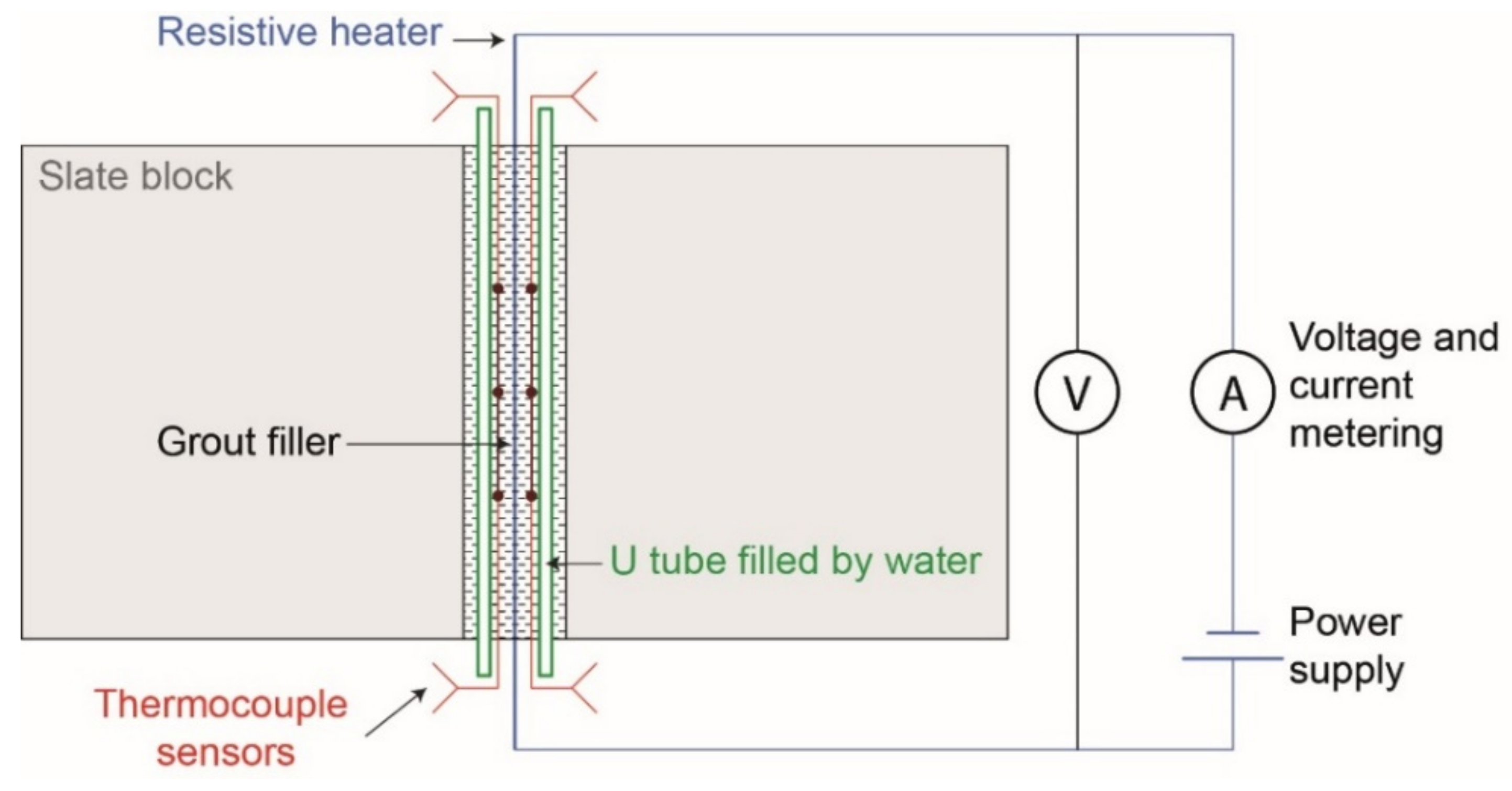
Tgr,∞ = 20 °C. This boundary condition can better represent the actual situation of the scale prototype located in a laboratory. The temperature into BHE domain is now calculated not only as an average along the three vertical ideal lines previously discussed, but also in specifically defined sample points, as sketched in
Figure 3.
The radial distance of all the sample points is r = 0.25 rb, except for the point TK4 that is located at the heater surface, namely for r = 0.1 rb.
Figure 4 presents the results of this numerical analysis. As expected, the temperature profile for the sample point on the heater (TK4) is higher than the others, although it presents the same slope, related to the thermal conductivity value. The other profiles, associated to sample points located all at the same radial distance (
r = 0.25
rb), almost overlap (with an error with respect to the nearly central point TK3 of less than 0.2 °C) in the previously discussed time range up to
τ = 15,000 s (
ln(
τ) = 9.62), except for the point TK1n. In fact, the temperature of the point TK1n is influenced by the boundary effects in the axial direction and the slope of its profile seems not useful for a proper calculation of the thermal conductivity.
As a consequence, in the scaled prototype the axial position of the thermocouple TK1n was modified (TK1), as presented again in
Figure 3, with a bigger distance from the boundary (0.07 m instead of 0.015 m).
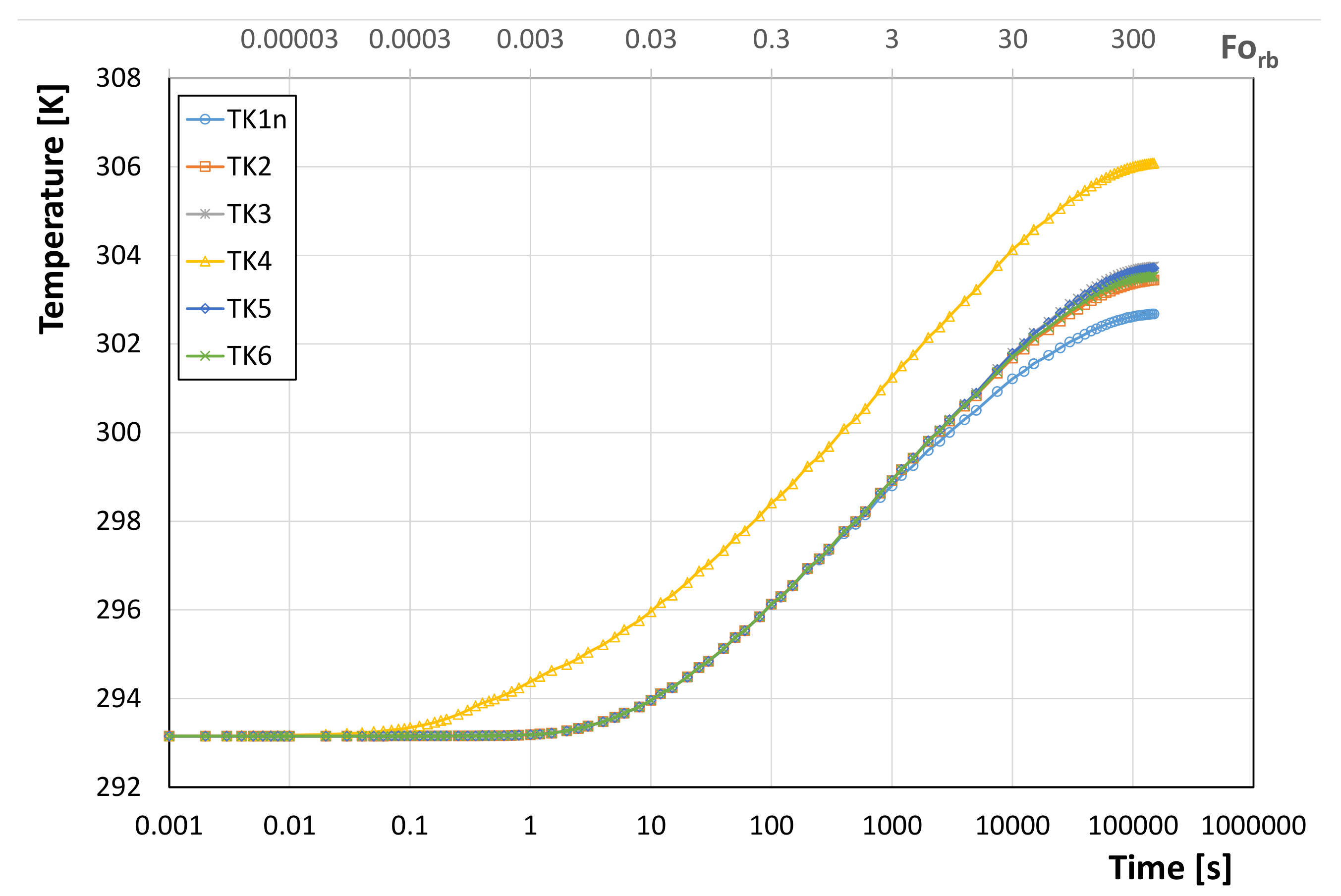
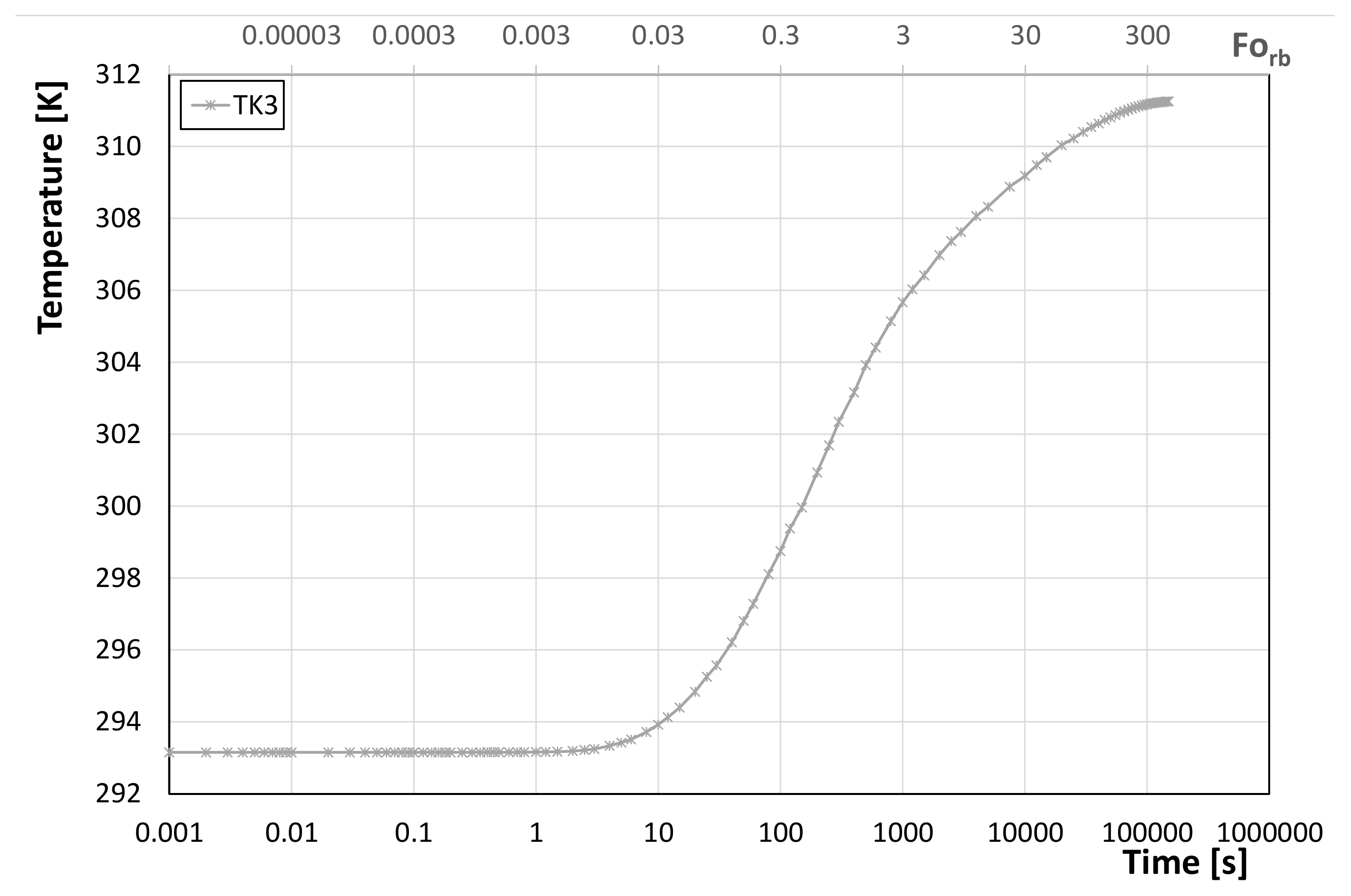
Finally, to have a more realistic idea of the actual behaviour of the scaled prototype, further simulations were carried out by imposing a different value of the grout thermal conductivity, namely
kgt = 0.8 W/m·K.
Figure 5 shows the corresponding temperature profile for the reference sample point TK3.
The trend plotted in
Figure 5 presents two different slopes: the first one, for approximately 5.5 <
ln(
τ) < 7, takes into account the thermal response of the medium near to the source, namely the simulated BHE; the second one, for
ln(
τ) > 7.5 and up to the suggested limiting value
ln(
τ) = 9.62
τ = 15,000 s) allows to estimate the slate/ground thermal conductivity.
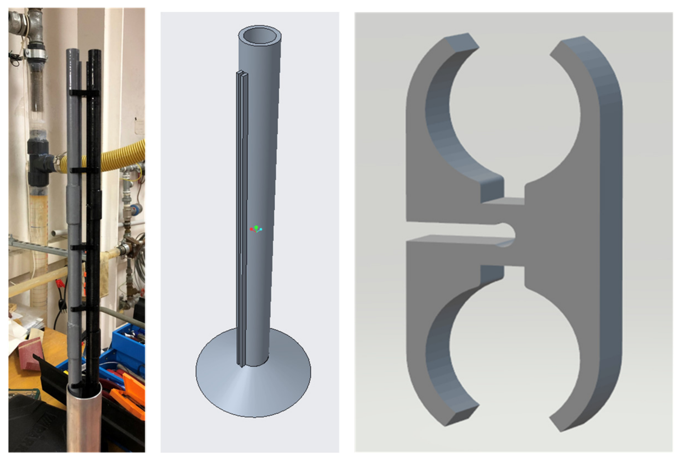
4. Experimental Apparatus
The scaled experimental set-up is aimed to represent the BHE and the surrounding ground volume. In particular, the test section is made by a slate block having dimensions 0.8 × 0.8 × 0.4 m (
Figure 6), axially perforated along the 0.4 m length (vertical direction). The cylindrical hole diameter is 40.5 mm. An aluminium tube, with external and internal diameters of 40 and 38 mm, respectively, was machined to fit the hole inside the rock block. The aluminum tube is aimed to simplify the disassembling of the test section, if necessary, when the hole is filled with grout. Tube thermal resistance demonstrated to be negligible compared to the grout and slate counterparts, as checked during Comsol simulations not reported here for the sake of brevity. Its small thickness and high thermal conductivity ensure negligible effects on the thermal behaviour of the assembly.
The present prototype incorporates the scaled borehole heat exchanger that includes the pipes (single or double U-pipe type), the resistive heating cable placed in the middle of the BHE, and a plurality of temperature sensors which are placed at known depths along the vertical direction and radial positions with respect to the heating cable (according to
Figure 3). The volume included among the plastic tubes, the heater, and the aluminium tube inside the borehole is filled by grout (
Figure 7).
The described BHE assembly represents an “all-in-one” heat exchanger, as shown in
Figure 8. To allow the positioning of the temperature probes at a known radial distance from the heater, the BHE plastic pipes are equipped with suitable ribbed parts. The electrical cable, that can provide the linear heating during the procedure, is maintained at the centre of the BHE by means of a proper spacer, in the present investigation realised by means of 3D additive manufacturing. The heat transfer rate can be conferred to the carrier fluid at the top ground surface (standard TRT) as well as by employing the electrical wire maintained at the centre of the BHE (innovative TRT experiment based on electric heating at the BHE axis). The carrier fluid circulation in the pipes can be guaranteed as well as the test can also be performed without any fluid circulation. The BHE pipes with suitable ribs (
Figure 9) were realised with a Cartesian-type 3D printer.
In the reduced scale experiment, the heating cable is realised by a resistance copper wire (Ø0.8 mm, a length of 0.42 m and heat shrink tube, shrink ratio 3:1). The 0.8 mm diameter resistance wire is characterised by a 0.97 Ω/m resistance per unit length. A constant heat transfer rate per unit length of about = 40 W/m has to be uniformly injected into the surrounding volume by the electrical wire. The cable is powered by means of a programmable, adjustable, switching, regulated DC 30 V/10 A power supply aimed to adapt the voltage and current parameters (model Rockseed RS310p, max voltage value 30 V, max current value 10 A DC).
The temperature sensors are armoured K-type thermocouples (Ø0.5 mm) and the temperature measurements are read and stored by a multi-channel and multi-function data logger 18bit acquisition board (model FieldLogger-Novus-HMI 512 K). The K-type thermocouples are accurately calibrated on 7 reference temperature values thanks to a thermostatic bath model Thermo Haake C25 and a reference PT100 class A thermometer inserted in the same calibration copper block. The sensor accuracy after calibration in the 5–60 °C range resulted in ±0.15 °C. Accuracy with respect to voltage and current at the power supply operating conditions (heat transfer rate per unit length of the heating cable ranging from 10 to 50 W/m) resulted to be within 0.5% of the readings.
Finally, the experimental apparatus, constituted by the slate block and all-in-one prototype heat exchanger, is located in a laboratory, maintained at a nearly constant temperature by means of an air conditioning system. The aim is to ideally realise, for the analysed domain, the imposed convective boundary condition with constant external temperature.
The reference thermal conductivity and heat capacity of slate were preliminary measured by means of a contact instrument, model Applied Precision Isomet 2114 conductivity meter, having an accuracy of 4%. Slate thermal properties were measured onto 10 different portions of the slate block. In addition, the slate thermal conductivity was also independently measured with a steady-state meter realised at the University of Genova (Unige), working on the principle of the one-dimensional Fourier law. Steady-state measurements were carried out on proper cylindrical slate samples (“disks”) cut from the same original rock volume.
Table 1 shows the thermal conductivity and heat capacity values obtained according to the above reference measurements, together with the uncertainty (standard deviation
σ (%)) due to instrument accuracy and repeated measurement differences.
Many factors can influence measurements performed on the same sample by different devices. Parameters such as the surface roughness of the sample face in contact with the probe, the size of the sample tested, possible fluctuations in ambient temperature and humidity, as well as possible non-homogeneities in the materials, can determine the non-uniformity of the same measurement. Exactly for this reason, it is advisable to repeat the analysis using measurement methods characterised by different approaches.
Before starting with the experimental campaign of the electrical TRT, some preliminary measurements were realised on the scaled prototype by means of an infrared camera, model Flir E6-XT. During the test, the heating cable located inside the scaled BHE was electrically powered and the surface temperature field was measured and corresponding images were captured.
Figure 10 shows an example of measurements of the temperature field at the top end of the heat exchanger as performed by the infrared camera. It is possible to visualise the circular shape of the temperature field around the heater due to the radial heat flux which confirms the assumptions on which the present analysis is based.
5. Inner Borehole Temperature Evolution
This section presents the preliminary measurements on the scaled prototype, realised by providing electrical power to the central cable in order to heat the borehole and the surrounding slate volume. At the same time, temperature values were measured by the K-type thermocouples, located in the scaled BHE according to
Figure 3. For each temperature sensor, a temperature vs. time profile can be obtained on a semi-logarithmic scale (
Figure 11).
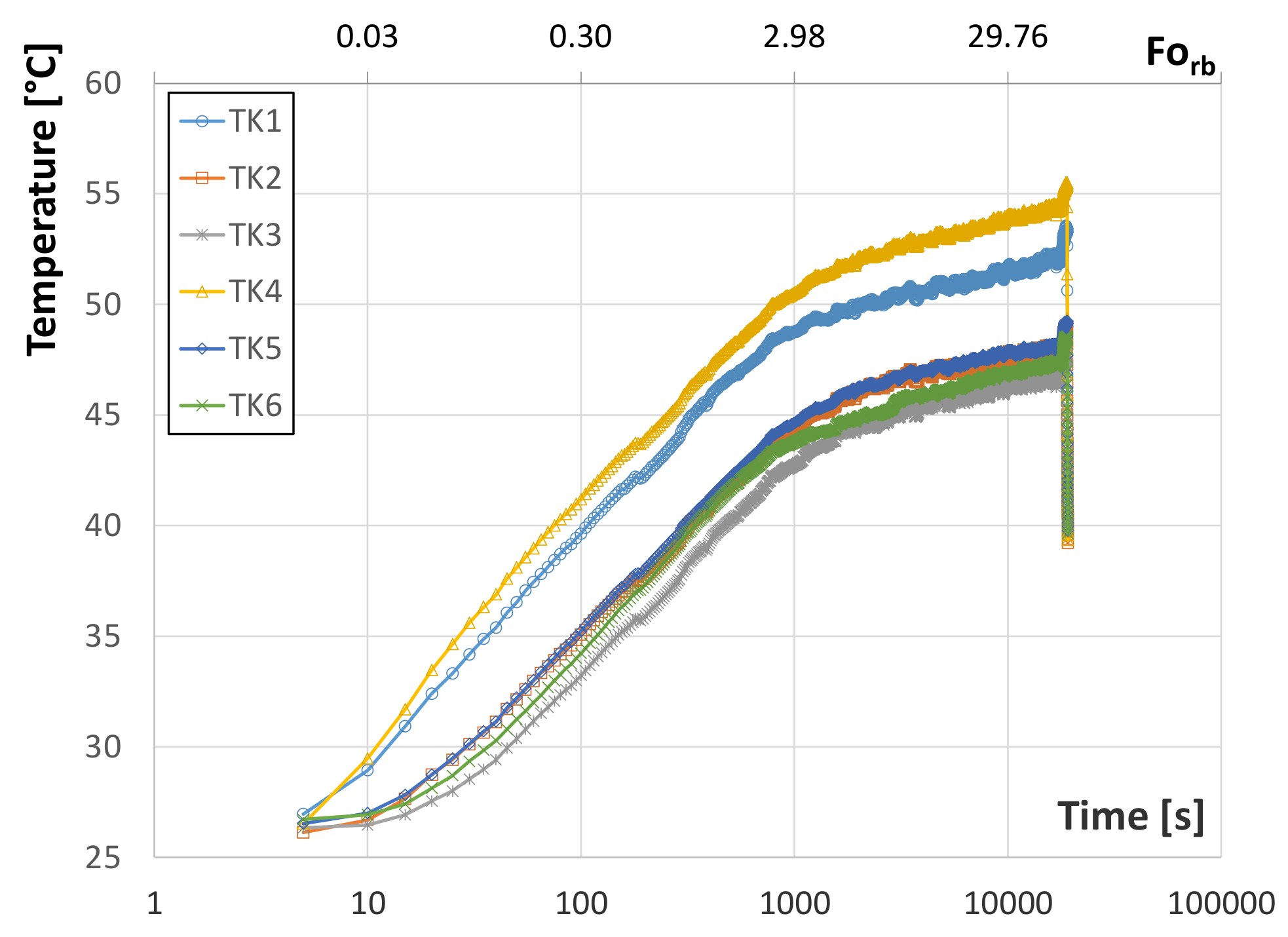
In particular,
Figure 11 shows the temperature profiles for one of the experimental tests carried out, during which a constant in time heat transfer rate per unit length is provided to the block (
= 38.86 W/m). According to the sketch of
Figure 3, the temperature sensor TK4 is located near to the electrical heater and the other sensors on the surface of the pipes. As a consequence, the temperature of TK4 is higher than the other, although keeping the same slopes. The temperature trends reveal that probably also the thermocouple TK1 has moved from the planned radial position toward the heater.
The medium around the heat sources is not homogenous because it is composed of the small volume representing the BHE and the big volume of the slate block that simulates the ground, considered as semi-infinite. Thus, the perturbation in the temperature field reaches first the BHE domain (for low
Forb) and later the slate one (for higher
Forb values). As a consequence, the temperature profile measured by the thermocouples shows different slopes for different
Forb ranges, in agreement with the simulated behaviour presented in
Figure 5. For this reason, two zones can be recognised on each graph, and only the second one can provide useful information to deduce the thermal conductivity of the slate/ground, namely for 7.5 <
ln(
τ) < 9.5.
Figure 12 focuses the attention on the “ground slope zone” and shows the linear temperature profiles recorded by the different sensors together with the trend lines, with their corresponding equations.
After estimating the slope of the linear profiles, according to it is possible to calculate the corresponding values of the ground thermal conductivity.
Table 2 summarises the main results related to the experimental test carried out. The agreement with the preliminary measured thermal conductivity values presented in 1 is good, especially comparing the results related to the central thermocouple TK6.
The error deviations between the estimated ground thermal conductivity average values provided by different methods were computed in terms of relative percentage error,
εi%, which is defined by the following equation:
The percentage relative error on the estimated average ground thermal conductivity provided by the experimental test with respect to the value measured by the Applied Precision Isomet 2114 conductivity meter resulted in +12.3%. It can be specified that deviations in the measurements of the same thermophysical property are also because the operating principles and related measurement methods on which each device is based are deeply different. Exactly for this reason, it is advisable to repeat the analysis using measurement methods characterised by different principles in order to increase the confidence level on the estimated property.


