Abstract
All over the world, the vehicles introduced now into the market are usually provided with EDRs (Event Data Recorders), intended to measure and record the parameters that characterise the vehicle motion in the pre-, during-, and post-accident phases. The EDRs are to facilitate the description and reconstruction of possible road accidents. They are patterned on aircraft “black boxes” (flight recorders). Many of them have simplified design, disregarding three (of six) vector components that describe the motion of the vehicle body solid. In the paper presented, the authors used simulation models built by themselves to represent motor vehicle dynamics and the reconstruction of vehicle trajectory and velocities based on records obtained from two EDR types: “aircraft” one (EDR1) and “simplified” one (EDR2). Using a simulation method, they examined the impact of the said simplifications mentioned above on the quality of reconstruction of vehicle motion for four typical manoeuvres in road traffic. The calculation results obtained for input data adopted to rep-resent a medium-class passenger car have shown that the simplifications may cause considerable reconstruction errors. This particularly applies to the manoeuvres where significant changes took place in the roll and pitch angles of the vehicle body solid (to which the EDR was fixed) or where the changes were characterised by absence of symmetry in the parameters that describe the manoeuvre and by the constant sign of the vehicle body roll angles.
1. Introduction
For more than 20 years, devices resembling aircraft’s “black boxes” and generally referred to as EDRs (Event Data Recorders) have been in use in motor transport. They are intended to record the parameters that describe vehicle motion, driver’s activities, state of vehicle’s systems, and sometimes current environmental conditions. The objective is to provide data concerning the course of road accidents (incidents), including the data useful for accident reconstruction.
Their scope of operation may be different, although some minimum requirements for the devices of this class have been set down by various normative documents and legal instruments. In this area, a fundamental role is played by a document issued under the auspices of NHTSA in the USA as early as 2006 [1], where the requirements for such devices have been laid down. In that document, the term EDR has been defined as follows: “(…) a device or function in a vehicle that records the vehicle’s dynamic time-series data during the time period just prior to a crash event (…) or during a crash event (…)”. Although without obligatorily requiring, that extensive document recommends vehicles to be equipped with such devices. In 2012, the NHTSA proposed a regulation [2], according to which EDRs should be installed in light-duty vehicles from 2014 on; however, it withdrew it in 2019 [3] with justifying that by the fact that an overwhelming majority of vehicles are already provided with EDRs meeting the requirements of [1]. In Europe, the legal regulations concerning this issue are just being implemented. Pursuant to Regulation (EU) 2019/2144 of the European Parliament [4], new vehicles will have to be equipped with EDR (from mid-2022 on). It should also be remembered that now EDRs are already installed in almost all new vehicles (in 2017, 99.6 % of all the light-duty motor vehicles newly manufactured in the USA were provided with EDRs, according to the document [3] mentioned above).
As already mentioned, the EDRs record the parameters that describe vehicle motion, driver’s operations on vehicle controls, state of vehicle’s systems, and sometimes current ambient conditions in the pre-, during- and post-collision phase. As regards vehicle motion, the basic signals recorded are those representing vehicle acceleration components, rotational speeds of vehicle wheels, data defining the angular position of the vehicle body (angles or components of the angular velocity of the vehicle body solid). The knowledge of these quantities, both in a direct and an appropriately processed form, makes it possible to obtain information about the dynamics and kinematics of motor vehicle motion in specific phases of the accident situation. The authors were mainly interested in the vehicle motion phase, which may be understood as the potential pre-accident situation. The main objective of the study was to estimate the possible accuracy of reconstruction of the time-series data that are important from the point of view of the analysis of motion, i.e., time histories of vehicle velocity and trajectory. The analysis has been carried out by taking into consideration the typical existing EDR solutions as regards the number of the parameters recorded that describe the motion of the vehicle body solid and the typical elements of vehicle manoeuvres (braking, lane-change, entering a turn, motion along a curve). The tests were carried out for a typical medium-class compact passenger car.
Many titles can be found in the literature that addresses the issues related to the accuracy of using EDR records. Most of them show a high usefulness of such solutions for accident analysis and present examples of their applications; see, e.g., [5,6,7,8].
There are also a few publications directly dealing with the accuracy of determining the parameters that describe the vehicle motion, but they mainly concern the strict collision phase and the determining of the vehicle velocity immediately before and after the collision or the vehicle velocity change during the collision, denoted by ΔV. As examples of such publications, [9,10,11,12,13,14,15,16] may be mentioned. A review of the materials showing the errors that occur when the pre- and post-impact velocities and ΔV are determined has been provided in [17], indicating the possible reasons for the inconsistencies having occurred.
Legal and technical issues related to using the EDRs have been discussed in [18] in the context of continuously rising vehicle autonomisation levels.
Also noteworthy are the publications describing research works in which the behaviour of drivers or the functioning of vehicle safety systems was assessed based on the EDR records of actual events. As an example, an attempt was made in the work reported in [19] to estimate the effectiveness of the operation of LDW (Lane Departure Warning) and LDP (Lane Departure Prevention) systems. A method of analysing the left-turn crashes with taking into account driver’s actions and based on EDR records of such incidents (as an input database) has been presented in [20]. In [21], EDR records of intersection crashes were used to propose an IADAS (Intersection Advanced Driver Assistance System).
There are only a few publications dealing with the vehicle motion in the pre-accident phase, i.e., in the phase when a hazardous situation is just arising. In [20], a trajectory approximation was used for the purposes of space-time analysis of a left-turn crash based on EDR records. EDR records of angular speeds of vehicle wheels, used as a basis for estimating the vehicle speed, have been analysed in [22]. The possibility of using this signal as a reliable source of information about the vehicle speed during braking has been highlighted. The research work was carried out for a vehicle provided with an air braking system. In [23], the velocity values obtained from EDR records were compared with the vehicle velocity measured by a self-contained device (V-Box). The velocity values obtained from CAN (EDR) were found to be in good conformity with the reference velocity. Similar conclusions can be found in [24]. In [25], the authors compare the EDR records with the V-box records during movement with rotation on a low friction road surface.
As regards the all-embracing analysis of vehicle motion based on EDR records of the motion dynamics, the [26] paper may be highlighted, where 3D transformations and integration of the accelerations recorded have been discussed as a method of obtaining information about the time histories of vehicle velocities and trajectory. Such a possibility has been shown, with potential difficulties having been emphasised. This possibility confirms to some extent the conclusions formulated by the authors of this paper in [27,28]. This paper presents the methods of determining the vehicle velocities and trajectory from EDR records on the one hand and, on the other hand, computational examples showing how some simplifications in EDRs’ design can affect the accuracy of the time curves being reconstructed. In these terms, the research works reported here are a direct continuation of those described previously in [27,28,29,30], but updated mathematical models of the test specimens adopted have been used in this case.
The fact that EDRs of various types are commonly used in present-day motor vehicles and the possibility of using their records for the reconstruction of vehicle motion and, on the other hand, scanty literature addressing these issues fully justify the undertaking of research in this field.
2. Materials and Methods
In the research presented, simulation calculational methods were used, where an experimentally verified model of motor vehicle dynamics and models of EDR records and of record processing algorithms were employed. A block diagram of the method has been shown in Figure 1. In the method adopted, the motion simulation results are taken as accurate (reference) values, and EDR records are simulated on these grounds (EDR model). Based on these records, time histories of the parameters describing the vehicle motion (velocity, position) are reconstructed with data processing algorithms (denoted by DPM, i.e., Data Processing Methods) being used. The difference between the reconstructed and accurate values is a measure of the reconstruction error. Individual elements of the method (vehicle dynamics model, EDR records model, and EDR record processing method, i.e., DPM) will be presented in subsequent subsections).
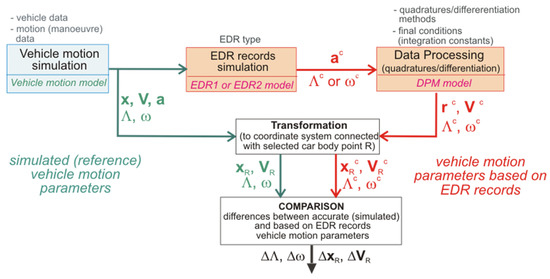
Figure 1.
Method of estimating the accuracy of reconstruction of vehicle motion, based on EDR records (a, V, ω, r, Λ—component vectors of: acceleration, velocity, angular velocity, position, angles, respectively).
2.1. Vehicle Dynamics Model
The tests were carried out for a KIA Ceed SW motor car, provided with a McPherson strut front suspension system with an antiroll bar. The suspension system (together with steering system components) is fastened to a subframe, which in turn is fixed to the car body solid. The left and right rear wheel suspension systems are independent of each other (apart from being coupled together by an antiroll bar). Each of them consists of a spring element (helical spring), shock absorber, two transverse arms, trailing arm, and lateral control rod. On both sides, the wheel suspension systems are fixed in a part to a steel drawpiece, which plays the role of a subframe.
A simulation model of this vehicle has been presented in publications [31,32,33] (Figure 2). It consists of 9 mass elements: vehicle body solid (treated as a rigid body), 4 material particles O1, O2, O3, and O4, where the vehicle’s “unsprung masses” have been concentrated (including road wheels in their translational motion), and 4 solids representing the rotating road wheels (exclusively in their rotational motion).
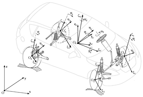
Figure 2.
Physical model of a two-axle motor vehicle with independent front and rear wheel suspension systems, together with the coordinate systems adopted.
The following coordinate systems have been adopted:
- -
- Oxyz—an inertial system, fixed to the road, with the Ox and Oy axes being horizontal and the vertical axis Oz pointing upwards;
- -
- OCxCyCzC—a moving non-inertial system, with its axes being respectively parallel to axes Ox, Oy, and Oz and with its origin situated at the centre of mass of the vehicle body solid Oc;
- -
- moving coordinate systems fixed to the rigid bodies of the model, i.e., body solid (OCξCηCζC) and four road wheels (O1ξ1η1ζ1, O2ξ2η2ζ2, O3ξ3η3ζ3, O4ξ4η4ζ4);
- -
- Auxiliary systems, facilitating the defining of transformation matrices.
To describe the translational motion of the solids and material particles of the model, the positions of the centres of mass (OC, O1, O2, O3, O4) of the said solids are used.
The axes Oiξi, Oiηi, Oiζi (i = C, 1, 2, 3, 4) are treated as the principal central axes of inertia of the corresponding rigid bodies.
The rotation of the vehicle body solid about the fixed point OC has been described with the use of “aircraft angles”, also referred to as “quasi-Euler angles” [34,35,36,37,38]:
- -
- Yaw angle ψC (rotation about the OCζC axis);
- -
- Pitch angle φC (rotation about the OCηC axis);
- -
- Roll angle ϑC (rotation about the OCξC axis).
The sequence of rotations has been adopted as identical to their listing order. The axes of individual rotations are treated as the principal central axes of inertia of the vehicle body solid.
The equations of motion have been derived with Lagrange equations of the second kind having been used. Prior to this, the following 14 generalised coordinates were adopted:
- q1 = xOC, q2 = yOC, q3 = zOC—coordinates defining the position of the centre of mass of the vehicle body solid (OC) in the inertial reference system Oxyz;
- q4 = ψC, q5 = φC, q6 = ϑC—coordinates describing the rotation of the vehicle body solid about its centre of mass OC; these are the quasi-Euler (aircraft) angles, i.e., yaw angle, pitch angle, and roll angle, respectively;
- q7 = ζCO1, q8 = ζCO2, q9 = ζCO3, q10 = ζCO4—coordinates describing the motion of points O1, O2, O3, O4 relative to the vehicle body solid in the direction of axis OCζC of the OCξCηCζC coordinate system; to these points, the “unsprung masses” of the suspension system are reduced;
- q11 = ϕ1, q12 = ϕ2, q13 = ϕ3, q14 = ϕ4—angles of rotation of road wheels (front left and right and rear left and right wheel, respectively).
In the model, the steering system flexibility and directional stability of road wheels have been taken into account. The tyre-road contact forces and moments have been described with the HSRI-UMTRI model [39,40] having been used, extended by adding the IPG-Tire model of transient states of tyres [41] in the form as adopted in paper [37].
The model has been experimentally verified as satisfactorily applicable to typical vehicle motion tests recommended by ISO or ECE, including the calculational part of the steady-state circular driving tests (ISO 4138, [42]), tests with step input applied to the steering wheel (ISO 7401, [43]), straight-line braking tests (UN ECE Regulation No 13, [44]), with the ABS being inactive.
2.2. Model of EDR Records
The EDR design solutions that can be met in reality differ from each other in the number of the recorded components of the vectors that define the vehicle position. In these terms, two characteristic EDR types have been distinguished (Figure 3). The devices of the first type (denoted herein by EDR1) are similar (within the scope as considered here) to flight recorders: they record three acceleration components, i.e., longitudinal one aw, lateral one ap, and “vertical” one aζ, and three angles, i.e., yaw angle ψC, pitch angle φC, and roll angle ϑC, or the corresponding angular velocities. The devices of the second type (denoted herein by EDR2) can be frequently met in motor vehicles and are a simplified version in comparison with the aircraft solution. The vehicle motion is treated as a two-dimensional one, with the parameters recorded being two acceleration components, i.e., longitudinal one aw and lateral one ap, and one angle, i.e., yaw angle ψC, or its time derivative, i.e., yaw velocity.
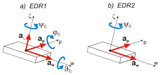
Figure 3.
Two EDR types: (a) EDR1 (6 parameters); (b) EDR2 (3 parameters).
The assumptions adopted in the mathematical model of acceleration sensors’ readings and the angular quantities have been described in dissertation [45] (and in [27] as well). An updated description can be found in [29,30]. Here, the main features of the description and fragments of its formal mathematical approach have been presented. The kinematic relations have been formulated by taking, as a basis, the model of kinematics shown in Figure 4. The vehicle motion is treated as a composition of translational motion of the centre OC of vehicle mass and of the rotation of vehicle body solid around point OC. Thus, 6 degrees of freedom of the vehicle body solid (3 translations and 3 rotations) are taken into account. One more reference system has also been added to the coordinate systems mentioned above (see Section 2.1):
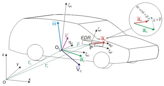
Figure 4.
Model if the kinematics of motion of a vehicle provided with an EDR, where the set of sensors is placed at point P; notation: r—position; V—velocity; a—acceleration in translational motion; ω—angular velocity; ε—angular acceleration.
PξPηPζP—a moving one, fixed to the EDR; the PξP, PηP, PζP axes define the directions of operation of the sensors of longitudinal and lateral acceleration and the yaw angle.
The vector symbols have the following meanings:
—Position of OC in the inertial system Oxyz;
—Position of point P in the inertial system Oxyz;
—Position of point P in the OCξCηCζC system;
—Angular velocity;
—Angular acceleration;
—Velocity of point OC;
—Acceleration of point OC;
—Acceleration of point P.
The kinematics of point P relative to the inertial system Oxyz is described as follows in matrix notation (point P is motionless in relation to the vehicle):
where the matrix of rotation A (from the OCξCηCζC system to the Oxyz system) has the form (4):
The positions of the sensors and their axes are defined by the positions of point P and coordinate axes of the PξPηPζP system. The position of this system relative to the OCξCηCζC one is defined by its translation by vector and by its rotation described by matrix C (see (5)). The rotations have been adopted in a way similar to that adopted previously, but in reverse order: ϑE (rotation about the longitudinal axis ξP), ϕE (rotation about the lateral axis ηP), and ψE (rotation about the “vertical” axis ζP)—see Figure 5b. Such a sequence of rotations is convenient because of the easy levelling of the sensor axes (oriented in relation to the vehicle).
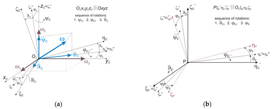
Figure 5.
Angular situation of the coordinate systems: (a) OCξCηCζC in relation to Oxyz; (b) PξPηPζP in relation to OCξCηCζC.
The basic component of the EDR model is the model of acceleration records. In this model, a system of transducer axes perpendicular to each other has been adopted, with the transducers being situated, as previously mentioned, freely in relation to the vehicle body. The fact has been taken into account that the acceleration transducers measure not only the real component of the acceleration of the EDR fixing point but also the pertinent components of the gravitational acceleration. Being inertia sensors, they measure a value proportional to the sum of the inertial and gravity force components acting along the sensor axis. The component resulting from the gravity force may be treated as the indication error.
Assuming a general formula for the sensor readings in the form (6):
We may write that vector ac is equal to:
where:
and g = [0, 0, −g]T—gravitational acceleration vector (g = 9.81 m/s2).
Vectors aPc and gc represent the acceleration of point P and gravitational acceleration, expressed in the reference system PξPηPζP (in the OCξCηCζC system attached to the vehicle, the same acceleration vectors are denoted by aP and gξ, respectively). The acceleration sensors’ readings have been graphically illustrated in Figure 6 (where the EDR2 unit has been used as an example for simplification).
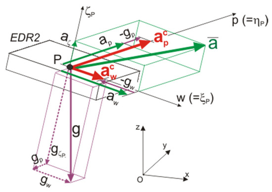
Figure 6.
Graphic interpretation of the longitudinal and lateral acceleration readings (awc and apc, respectively).
In the description presented, the sensors have been assumed to be free of intrinsic errors. A model applicable to the readings describing angular position (angles or angular velocities) has been developed as well. Its formal description can be found in [27,45].
2.3. Reconstruction of Motion (DPM Model)
The reconstruction of motion consists of appropriate (for the specific recorder configuration, e.g., EDR1 or EDR2) processing of the recorder’s output signals. A schematic diagram of the data processing procedure has been shown in Figure 7. The procedure is based on the integration of acceleration records transformed to the inertial system attached to the road. The numerical integration ([46,47]) is carried out from a definite final instant corresponding to a known vehicle position and velocity (e.g., post-accident vehicle position specified by witnesses). If possible, transducer readings are adjusted by adding the values of gravitational acceleration components (Δac = −gc, see Equation (7)). The results of successive quadrature operations define, as appropriate, the velocities and positions of point P of fixing the EDR, expressed in the inertial system Oxyz. Afterwards, they can be transformed in order to obtain time histories of the velocities and trajectories of any point in the vehicle body.
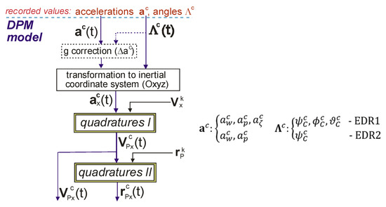
Figure 7.
Schematic diagram of the processing of data recorded by the EDR: ax, Vx, rx,—vectors of acceleration, velocity, and position, respectively, in the inertial reference system Oxyz; Vk, rk—velocity and position at the final instant; “P” in the subscript indicates the values for point P of fixing the EDR; ψCc, φCc, ϑCc—values of angles ψC, φC, ϑC, determined from EDR records.
Figure 7 shows a schematic diagram of the processing of data produced by a recorder of angle values. In such a case, the angular velocities are obtained by numerical differentiation of the angles. If, on the contrary, angular velocities are recorded then the angle values are obtained by differentiation of time histories of the velocities.
3. Results
The calculations were carried out for data of a medium-class compact passenger car KIA Ceed SW, i.e., mass 1870 kg, wheelbase 2.65 m, and distance between the centre of vehicle mass and the front axle 1134 m, with simulating vehicle motion on dry, level, and ideally even road surface with good tyre-road adhesion (equivalent to asphalt concrete). A specific vehicle motion (manoeuvre) was forced by applying control signals representing time histories of the steering wheel angle and brake pedal effort (in the case of braking). For “constant sped” curvilinear motion tests, a driver model (driving torque controller) was activated to maintain constant vehicle speed.
Four typical vehicle motion cases were examined:
- Straight-line braking;
- Lane-change manoeuvre;
- Entering into a turn;
- Driving in a roundabout (circular motion).
In each of the cases, various intensities of the manoeuvres (measured by the level of longitudinal or lateral acceleration) were applied.
Both EDR types mentioned in Section 2.2 were taken into consideration: EDR1 (6 parameters of the motion) and EDR2 (3 parameters of the motion). For the analysis, an option was adopted where angles (instead of angular velocities) were used to define the angular position of the vehicle body solid. Moreover, to avoid the introduction of additional disturbing factors that might affect the calculation results, an assumption was made that the EDR sensors were placed at the centre of vehicle mass (see Figure 4, P = OC) and the motion of the centre of the vehicle mass was analysed (see Figure 1, R = P = OC). In addition to the above, an assumption was also made that the sensors had been calibrated for the vehicle standing on a horizontal road and loaded as in the tests. The frequency of recording the parameters under analysis was assumed as 20 Hz.
3.1. Straight-Line Braking
Figure 8 and Figure 9 show the analysis results obtained for the case of braking the vehicle from an initial speed of 90 km/h with a deceleration of about 6 m/s2 (this is approximately equal to the absolute value of the longitudinal acceleration of the centre of the vehicle mass). The vehicle braking was caused by applying a force to the brake pedal, where the driver reaction time and the reaction of braking system components were reflected in the time history of the brake pedal force. Figure 8a shows the actual (simulated, considered as “accurate”) value of longitudinal acceleration aPξ and the value recorded by the EDR (awc). The difference between them (denoted by φawc) resulted from variations in the pitch angle ϕ1 (see Figure 8b).
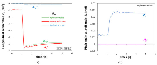
Figure 8.
Straight-line braking. Initial vehicle velocity 90 km/h, deceleration level 6 m/s2. Time histories of: (a) longitudinal acceleration (accurate values and EDR sensor indications); (b) car body pitch and roll angles (accurate values).
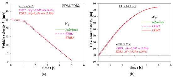
Figure 9.
Straight-line braking. Initial vehicle velocity 90 km/h, deceleration level 6 m/s2. Reconstruction of time histories of: (a) vehicle velocity; (b) distance travelled by the vehicle. Reconstruction based on EDR1 and EDR2 records.
Figure 9 shows the reconstruction results obtained by using recorders of both types (EDR1 and EDR2). The time histories of vehicle velocity and position were reconstructed “backwards”, i.e., from the known final vehicle position and velocity to the initial instant of the simulation of the vehicle motion. The data presented in Figure 9a,b concern vehicle velocity and position, respectively. The differences that can be seen at the beginning of the velocity and position curves illustrate the reconstruction errors, i.e., errors of determining the initial velocity (ΔV0) and distance travelled (ΔS).
Very good conformity can be seen between the reconstructed and accurate values for the EDR1 device. This is thanks to the fact that in this case, the accelerometer indication error Δawc is automatically corrected in the EDR1 calculation algorithm, because the vehicle pitch angle, which causes this error, is known and, in consequence, the value of this error can be determined. In the case of the EDR2 device, the pitch angle is not known and the acceleration signals being integrated are burdened with the error arising from that. In the case under consideration, this translates into an overestimation of the values of initial velocity and distance travelled by the vehicle.
Analysis results were obtained for more cases, differing from each other in the pre-set initial vehicle velocity (50, 90, and 140 km/h) and braking intensity (deceleration level of about 2, 4, 6, and 8 m/s2) have been summarised in Table 1. Additionally, the errors in estimating the initial velocity and stopping distance of the vehicle have been directly shown in the absolute and relative form in Figure 10 and Figure 11.

Table 1.
Straight-line braking. Summary of the accurate and reconstructed values of initial velocity and stopping distance of the vehicle for different preset levels of the initial velocity (50, 90, and 140 km/h) and braking intensity (deceleration level of about 8, 6, 4, and 2 m/s2).
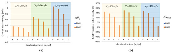
Figure 10.
Straight-line braking. Errors of the reconstruction of the initial velocity of the vehicle motion: (a) in the absolute form; (b) in the relative form.
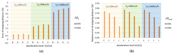
Figure 11.
Straight-line braking. Errors of the reconstruction of the vehicle stopping distance: (a) in the absolute form; (b) in the relative form.
In the case of EDR1, the errors are practically negligible (they arise from different integration frequencies in the vehicle motion simulation process and during the reconstruction of vehicle motion parameters). For the initial velocity and EDR2 records, growth in the relative and absolute errors with increasing braking intensity can be seen. Such an effect may be explained by the fact that an increase in braking deceleration values results in a growth in the pitch angle and, in consequence, in the longitudinal acceleration estimation error, which translates into bigger errors of the integration output signals. A somewhat different situation takes place for stopping distance errors. In this case, the absolute errors do not depend so visibly on deceleration values and a relatively more significant role is played by the initial velocity value. However, the situation becomes similar to that observed for velocity errors already when relative errors of estimating the distance travelled are concerned: higher braking intensity results in bigger, in percentage terms, relative errors of estimating the braking distance.
Nevertheless, it should also be emphasised that, from the practical point of view, the reconstruction errors in the case of EDR2, although being bigger, are still not very serious (they did not exceed 3 % in the tests under consideration). This is significantly influenced by the general inertial characteristics of the vehicle body and by the design and stiffness of the vehicle suspension system, which translate into relatively small changes in the pitch angle of the vehicle during the braking manoeuvre. In similar research works described in [27,28], the errors in estimating the initial vehicle velocity and stopping distance were bigger (even twice). Those results were obtained for another passenger car, which was also more susceptible to vehicle body pitch and roll.
3.2. Vehicle Lane-Change Maneuvre
In this test, the vehicle is to perform a manoeuvre similar to the lane-change one. The test manoeuvre was forced by applying a control signal representing the steering wheel angle in the form of one period of sinusoidal input (with reference to the Sinusoidal Input test according to ISO 7401) with a reaction time of 1 s. The sinusoid parameters (period and amplitude) were selected individually for a specific vehicle test velocity (50, 90, 140 km/h) so that the vehicle virtually changed a lane about 3.5 m wide (i.e., the centre of vehicle mass, often referred to as centre of gravity—C.G., changed its lateral position by about 3.5 m) and for a chosen intensity of the manoeuvre (low, medium, or high, with the manoeuvre intensity being defined by the level of the maximum lateral C.G. acceleration). The total manoeuvre observation time was 5 s. Figure 12 and Figure 13 show the results obtained for the vehicle moving with an initial velocity of 90 km/h and performing the manoeuvre with an intensity defined as “medium” (with the maximum lateral acceleration level of about 5 m/s2). Similarly, as in the case of braking, Figure 12a shows the actual (accurate) value of the lateral acceleration aPη and the value recorded by the EDR apc. The difference between these two values (denoted by Δapc) mainly results from changes in the roll angle ϑC and, to a lower degree, from changes in the pitch angle φC, shown in Figure 12b.
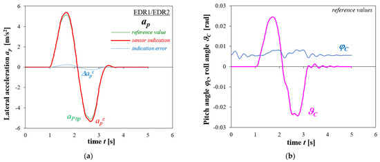
Figure 12.
Lane-change manoeuvre, “medium” intensity level. Initial vehicle velocity 90 km/h. Time histories of: (a) lateral acceleration (accurate value and EDR sensor indication); (b) car body pitch and roll angles (accurate).
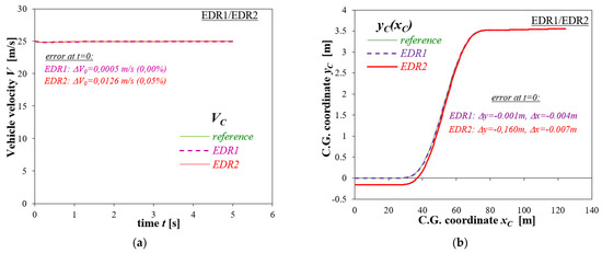
Figure 13.
Lane-change manoeuvre, “medium” intensity level. Initial vehicle velocity 90 km/h. Reconstruction of: (a) vehicle velocity; (b) vehicle body C.G. trajectory. Reconstruction based on EDR1 and EDR2 records.
Figure 13 shows the results of reconstruction of a 5 s time period of the vehicle motion, obtained by using recorders of both types (EDR1 and EDR2). As previously, the time histories of vehicle velocity and position were reconstructed “backwards”, i.e., from the known final vehicle position and velocity to the initial instant of the simulation of the vehicle motion. The data presented in Figure 13a,b concern vehicle velocity and C.G. trajectory, respectively. The differences that can be seen at the beginning of the velocity and position curves illustrate the reconstruction errors, i.e., errors of determining the initial velocity (ΔV0) and distance travelled (ΔS).
Similarly, as in the case of braking, very good conformity can be seen between the reconstructed and accurate values for the EDR1 device. The reason for this fact is identical. The accelerometer indication errors are automatically corrected because the vehicle pitch and roll angles are known. In the case of the EDR2 device, the said angles are not known, and the acceleration signals being integrated are burdened with the errors arising from that. In the case under consideration, this translates into an overestimation of the values of the lateral vehicle displacement and a velocity estimation error.
Analysis results obtained for more cases, differing from each other in the pre-set initial vehicle velocity (50, 90, and 140 km/h) and manoeuvre intensity (three lateral acceleration levels: about 2.4–2.5, 5.0–5.4, and 7.1–8.2 m/s2), only for the EDR2 device, in this case, have been summarised in Table 2. Additionally, the errors of estimating the initial velocity and distance travelled by the vehicle during the manoeuvre have been directly shown in the absolute and relative form in Figure 14. In quantitative terms, these errors may be considered quite small (tenths of percentage units), the reasons for which may be sought, as previously, in small changes in the roll angle (in this case) and in the resulting small errors of estimating the lateral acceleration. However, the trend of these errors rising with the intensity of this manoeuvre can be noticed here as well.
Table 2.
Lane-change manoeuvre. Summary of the simulated (accurate) and reconstructed values of initial vehicle velocity, initial position estimation error, and distance travelled by the vehicle for different preset levels of the initial velocity (50, 90, and 140 km/h) and manoeuvre intensity (low, medium, high). Manoeuvre observation time: 5 s.
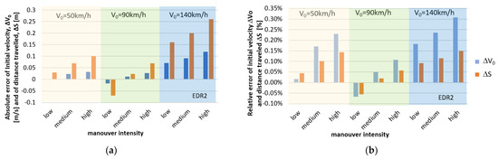
Figure 14.
Lane-change manoeuvre. Errors of the reconstruction of the initial vehicle velocity and of the distance travelled by the vehicle: (a) in the absolute form; (b) in the relative form. Reconstruction based on EDR2 records.
3.3. Entering a Turn
The test consists in dynamic making the vehicle under test follow a curve. Such a manoeuvre was forced by applying a control signal representing a constant steering wheel angle preceded by a linear angle raising period (with reference to the Step Input test according to ISO 7401), where the steering wheel angle values were selected individually for a specific vehicle test velocity (50, 90, 140 km/h) so that the vehicle performed the manoeuvre with various intensities defined by the maximum lateral C.G. acceleration level in the steady phase of the motion (2, 4, 6, 8 m/s2). The angle-raising time was so adopted that the steering wheel rising-rate fell within the limits stipulated by the said ISO standard. The total manoeuvre observation time was 5 s. In this case, only the results obtained by using the EDR2 recorder have been presented (for the EDR1 device, the reconstruction results were practically identical with the accurate data). The reconstruction results have been presented in Figure 15, Figure 16, Figure 17 and Figure 18, in the form as before, for two options of the manoeuvre, i.e., for initial velocities of 50 km/h and 140 km/h, and for the maximum lateral acceleration level of about 8 m/s2.
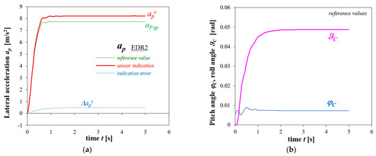
Figure 15.
Entering a turn, intensity level 8 m/s2. Initial vehicle velocity 50 km/h. Time histories of: (a) lateral acceleration (accurate values and EDR2 sensor indications); (b) car body pitch and roll angles (accurate values).
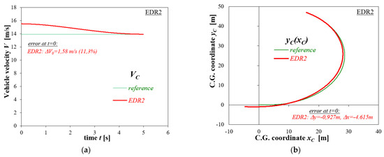
Figure 16.
Entering a turn, intensity level 8 m/s2. Initial vehicle velocity 50 km/h. Reconstruction of: (a) vehicle velocity; (b) vehicle C.G. trajectory; reconstruction based on EDR2 records.
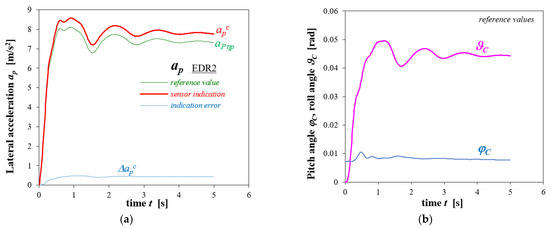
Figure 17.
Entering a turn, intensity level 8 m/s2. Initial vehicle velocity 140 km/h. Time histories of: (a) lateral acceleration (accurate values and EDR2 sensor indications); (b) Car body pitch and roll angle values (accurate).
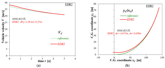
Figure 18.
Entering a turn, intensity level 8 m/s2. Initial vehicle velocity 140 km/h. Reconstruction of: (a) vehicle velocity; (b) vehicle C.G. trajectory; reconstruction based on EDR2 records.
Results of all the tests carried out with entering a turn have been presented in Table 3. For better illustration of the differences obtained, the errors of estimating the initial velocity and distance travelled by the vehicle during the manoeuvre have been directly shown in the absolute and relative form in Figure 19; Figure 20 presents the initial positions of the centre of vehicle mass (C.G.), reconstructed with EDR2 records being used.
Table 3.
Entering a turn. Entering a turn. Summary of the simulated (accurate) and reconstructed values of initial vehicle velocity, errors of estimating the initial vehicle position, and distance travelled by the vehicle for different pre-set levels of the initial velocity (50, 90, and 140 km/h) and manoeuvre intensity (2, 4, 6, 8 m/s2). Manoeuvre observation time: 5 s.
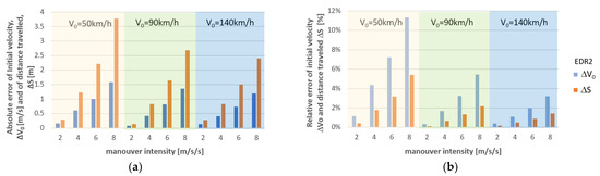
Figure 19.
Entering a turn. Errors of the reconstruction of the initial vehicle velocity and of the distance travelled by the vehicle: (a) in the absolute form; (b) in the relative form. Reconstruction based on EDR2 records.
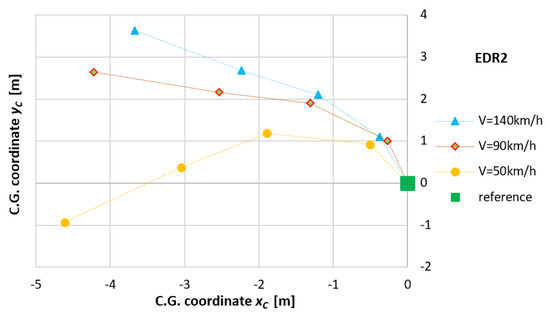
Figure 20.
Entering a turn. Initial positions of the centre of vehicle mass (C.G.), reconstructed with EDR2 records being used.
When analysing the results obtained for this manoeuvre, it should be noted that the reconstruction errors are here markedly bigger than those occurring in the case of the lane-change manoeuvre. For the motion, parameters range under consideration, the errors of estimating the initial velocity or distance travelled by the vehicle reach from a few to even more than ten percent (Figure 19). The initial vehicle position obtained from the reconstruction may differ from the actual (accurate) one by a few meters (Figure 20). Noteworthy is the fact that the manoeuvre observation time was identical for both manoeuvre types (5 s). The reasons for such an effect may be sought in the fact that, similarly as it is in the case of braking and longitudinal deceleration, no reversal of the sign of vehicle acceleration and its error takes place (Figure 15 and Figure 17), contrary to the situation that takes place during the lane-change manoeuvre, where the errors of the reconstruction (acceleration quadrature operations) generated in one phase of the manoeuvre are partly compensated by the reconstruction errors generated in the other manoeuvre phase.
Another factor worth consideration is the impact of manoeuvre intensity. Here, similarly as in other manoeuvres, the errors increase with rising manoeuvre intensity; this may be directly associated with an increase in the errors of the EDR acceleration records due to growing vehicle body pitch and roll angles.
The last regularity that can be noticed is a decrease in error values with increasing vehicle velocity, which distinguishes this manoeuvre from a similar case (in terms of absence of reversal of the acceleration sign), i.e., from the straight-line braking. To explain this finding, it is worth noticing that, apart from the initial phase of the manoeuvre, the vehicle motion under analysis is similar to the steady-state motion along a circle. Therefore, it is worth paying attention to another variable that characterises the vehicle motion, i.e., the yaw angle. Figure 21 presents the data collected that show the “angular distance” travelled by the vehicle in every case. When comparing the data plotted in this graph with the reconstruction errors presented previously in Figure 19, their qualitative convergence can be noticed: the higher the velocity, the smaller the change in the yaw angle in the manoeuvre under consideration. Based on the said qualitative convergence, a hypothesis may be formulated that the value of errors, especially the errors of the vehicle trajectory, are affected by the “angular distance” travelled by the vehicle. This aspect will be presented in broader terms in the next example, where the steady-state circular motion will be analysed.
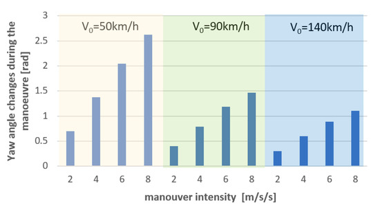
Figure 21.
Entering a turn. Range of changes in the vehicle yaw angle during the manoeuvre.
3.4. Driving in a Roundabout (Circular Motion)
In such a test, the vehicle is driven with a constant speed along a curvilinear path close to a circle (to some extent, the test conditions are close to those of the ISO 4148 test [42]). The manoeuvre is forced by applying a constant non-zero steering wheel angle. The test parameters (vehicle speed, steering wheel angle) were so selected that, on the one hand, the vehicle moved with a prescribed lateral acceleration (2, 4, or 6 m/s2) and, on the other hand, the vehicle path was in accordance with the roundabouts that can be met in real roads [48] (and simultaneously the actual radius of the vehicle path was in conformity with the recommendations of the said ISO 4138 standard). Actually, the vehicle path radius was set at about 30 m, and the values of the vehicle speed on the virtual traffic circle were about 30, 40, and 50 km/h. The manoeuvre was considered as completed when the vehicle travelled a “full circle”, i.e., the vehicle yaw angle changed by 2π in the simulation.
This time, the trajectories reconstructed (“backwards” from the final vehicle position) have been presented as the first thing (see Figure 22). Figure 23 shows a reconstruction of the time history of the vehicle speed (“backwards” from the final instant). The direct causes of the visible differences between the accurate and reconstructed vehicle trajectories and speed vs. time curves mainly lie in errors of the EDR2 acceleration records (differences between the accurate and recorded acceleration values) shown in Figure 24.
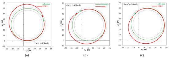
Figure 22.
Driving in a roundabout, R = 30 m. Reconstruction of vehicle body C.G. trajectory based on EDR2 records. Lateral acceleration level: (a) 2 m/s2; (b) 4 m/s2; (c) 6 m/s2. “●”—start of the reconstruction (end of the motion under analysis); “♦”—end of the reconstruction (reconstructed initial position); grey dotted lines represent edges of the roundabout carriageway 6 m wide.
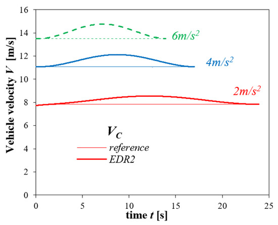
Figure 23.
Driving in a roundabout, R = 30 m. Reconstruction of vehicle C.G. speed based on EDR2 records for three lateral acceleration levels: 2 m/s2; 4 m/s2; 6 m/s2.
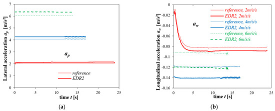
Figure 24.
Driving in a roundabout, R = 30 m. Comparison between time histories of accurate values and EDR2 sensor readings of: (a) lateral acceleration; (b) longitudinal acceleration.
At first, the differences between the accurate and reconstructed curves can be found to be similar to each other in qualitative terms: the differences increased in the first phase of the manoeuvre and decreased afterwards. This resulted in very good conformity between the accurate and reconstructed value of the vehicle speed and in quite good conformity between the accurate and reconstructed initial vehicle position (the vehicle C.G. coincided with the accurate trajectory). Here, reference may be made to the hypothesis proposed in the previous subsection about the dependence of errors on the “angular distance” travelled by the vehicle and, in consequence, about the “periodicity” of the errors. Therefore, the vehicle speed and position errors have been presented in Figure 25 not in the time domain but as functions of changes in the angular position (yaw angle) within the range from the final position (for which the change is equal to zero) to the initial position (where the change is equal to −2π). Additionally, the estimated values of the vehicle body C.G. path radius and the vehicle yaw velocity have been presented in Figure 26.
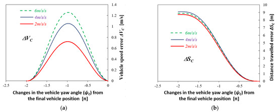
Figure 25.
Driving in a roundabout, R = 30 m. Errors of: (a) vehicle body C.G. speed; (b) vehicle body C.G. distance travelled as a function of changes in the vehicle yaw angle (zero—vehicle final position, −2π—vehicle initial position).
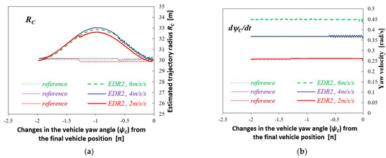
Figure 26.
Driving in a roundabout, R = 30 m. (a) Estimated radius of the vehicle body C.G. trajectory; (b) Yaw velocity as a function of changes in the vehicle yaw angle (zero—vehicle final position, −2π—vehicle initial position).
It can be seen that on the interval from zero to −π, the speed reconstruction error is increasing; in consequence, the rate of growth in the error of estimating the distance travelled is increasing as well. On the interval where the vehicle has already “turned back”, i.e., from −π to −2π, the speed reconstruction error is decreasing to values close to zero; the distance error is still increasing, but the growth rate is decreasing. Since the vehicle yaw velocity is approximately constant (Figure 26b), the changes in the reconstructed vehicle speed value translate into changes in the reconstructed trajectory radius value (Figure 26a), i.e., growth in the radius on the yaw angle range from 0 to −π and decline on the range from −π to −2π.
Noteworthy is also the fact that the reconstruction errors are also affected by the error in estimating the longitudinal acceleration (Figure 24b). In the example presented, this can be seen, e.g., in Figure 25b and Figure 26a, when the cases with 4 m/s2 and 6 m/s2 are compared with each other. For the manoeuvre with 6 m/s2, the longitudinal acceleration level, in terms of its absolute value, is lower than that for the manoeuvre with 4 m/s2 (see Figure 24b). This has contributed to the fact that in spite of a higher level of lateral acceleration, the errors in estimating the distance travelled are here somewhat lower (see Figure 25b). Similarly, the radius of the reconstructed trajectory is also somewhat smaller (see Figure 26a).
It may be assumed that during the next circling, this situation may repeat itself again and again. To illustrate this effect, Figure 27 presents the vehicle trajectory and speed curves for the simulation of driving in a runabout with a speed of about 50 km/h (lateral acceleration level of 6 m/s2) for an “angular distance” exceeding the value of 2π as shown previously (the yaw angle was now 3.02 rad at the initial instant and 14.03 rad at the final instant, i.e., it changed by 11.01 rad ≅ 3.5π). The vehicle speed error “oscillates” with a period of 2π, the distance error is increasing cycle after cycle, and the reconstructed trajectory “shifts” by a certain distance with every cycle.
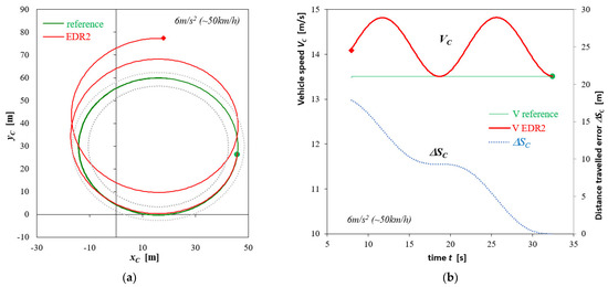
Figure 27.
Driving in a roundabout, R = 30 m. Lateral acceleration level 6 m/s2 (vehicle speed ca. 50 km/h). Reconstruction based on EDR2 records of: (a) vehicle body C.G. trajectory; (b) vehicle body C.G. speed and error of the distance travelled. “●”—start of the reconstruction (end of the motion under analysis); “♦”—end of the reconstruction (reconstructed initial position); grey dotted lines represent edges of the roundabout carriageway 6 m wide.
In the context of the above findings, therefore, attention should be paid to the fact that at the reconstruction of manoeuvres like the one discussed here (or the entering a turn, as discussed previously), a factor of considerable importance for the magnitude of errors in the event reconstruction based on records obtained by using EDR2-like devices is a change in the yaw angle during the manoeuvre. Depending on the scope of the change, the errors may be small or very big. For the vehicle trajectory, the positions determined by reconstruction may so differ from the actual ones that correct interpretation of the situation under analysis would become impossible (errors would be of the order of several meters, such that the vehicle position thus determined would be situated e.g., outside of the road area or of any realistic vehicle trajectory).
4. Discussion
The results obtained have been discussed in detail immediately after their presentation. To synthesise the findings in the context of the accuracy of the reconstruction of vehicle motion, the following may be stated.
- -
- In the case of the EDR1-type devices (recording 6 vector components that describe the vehicle motion), the reconstruction results are practically identical with the reference (accurate) data.
- -
- In the case of the EDR2-type devices, the velocities and trajectories may both slightly and significantly differ from the accurate data.
- -
- The qualitative nature of the accident reconstruction errors depends, inter alia, on the vehicle motion type. In the case of straight-line braking, errors arise in determining the initial vehicle velocity and the distance travelled; when curvilinear motion is analysed, deviations from the accurate vehicle trajectory mainly occur.
- -
- In quantitative terms, the errors may be influenced by the intensity of the manoeuvre. In general, the higher intensity is connected with larger reconstruction errors (arising from stronger angular movements of the vehicle body and, in consequence, from bigger errors in the accelerations recorded).
- -
- Another factor that has an impact on the accuracy achieved is the period of time (or the length of the distance travelled) for which the vehicle motion is reconstructed. For short-duration manoeuvres (lasting less than 5 s), good accuracy can be achieved, even if the EDR2 devices are used (with reservations formulated in other conclusions). However, the errors increase with the increasing length of the period for which the motion is reconstructed. Attention should also be paid to the effects reported for the case of circular motion, i.e., a kind of cyclicity of the reconstruction errors.
- -
- A quantitative influence on the accuracy may be exerted by the design and operational features of the vehicle. This concerns the properties that have a considerable impact on the angular movements of the vehicle body solid. The features of particular importance may be suspension system characteristics (e.g., suspension system design, spacing, and stiffness of springs, dry friction, etc.).
To some extent, especially as regards the quantitative findings, the results presented confirm the conclusions expressed in [27,28,29] as well as in [26]. The directions of further research on the accuracy of reconstruction of vehicle motion based on records obtained from EDR-type devices, concerning such issues as the impacts of current load and design features of the vehicle, accuracy of the measuring and recording apparatus, angular positioning of EDR sensors, or EDR configuration (e.g., recording of angular velocities instead of angles, recording frequency), can also be formulated.
5. Conclusions
The large-scale introduction of automotive “black boxes” into service will potentially bring many benefits. It will increase the resource of information about the course of an accident and will provide knowledge of the parameters of vehicle motion. Other advantages may consist in preventive influence on the driver, who will be less prone to risky behaviours in road traffic. The EDR solutions offered now in the automotive market are often a simplified version of the solutions having been used in aviation for many years. In the EDRs offered in the market, apart from those intended for research applications, the vehicle motion is generally treated as two-dimensional (as it is in the EDR2).
In the research carried out, the interest was focused on the concept of the EDR, without addressing the problems related to the measuring and recording apparatus (such as intrinsic sensor errors or errors arising in the recording process). The calculations carried out have shown that the said simplifications may result in significant errors in the reconstruction of vehicle motion, sometimes totally disqualifying the reconstruction results. This mainly applies to the reconstruction of vehicle trajectory; nevertheless, a result significantly differing from the actual value is also possible when the vehicle velocity is reconstructed. The basic reason for that lies in the fact that the devices of the EDR2 type do not provide information about some angular movements of the vehicle body solid, i.e., the pitch and roll angles. In the case of the EDR1 devices, no considerable reconstruction errors have been revealed.
Author Contributions
Conceptualization, M.G. and Z.L.; methodology, M.G. and Z.L.; software, M.G. and Z.L.; validation, M.G. and Z.L.; formal analysis, M.G. and Z.L.; investigation, M.G. and Z.L.; writing—original draft preparation, M.G. and Z.L.; writing—review and editing, M.G. and Z.L. All authors have read and agreed to the published version of the manuscript.
Funding
This research received no external funding. APC was funded by Warsaw University of Technology.
Institutional Review Board Statement
Not applicable.
Informed Consent Statement
Not applicable.
Data Availability Statement
Not applicable.
Acknowledgments
The simulation model of motor vehicle motion and dynamics, used in this work, was built during the execution of a project carried out by the Faculty of Transport, Warsaw University of Technology (WUT) to commission of ETC-PZL Aerospace Industries Ltd. (being now owned by a US company Environmental Tectonics Corporation and AIRBUS Poland S.A.). The superior goal of the project was to build a simulator of driving emergency service vehicles within project No O ROB 0011 01/ID/11/1 “Simulator of driving emergency service vehicles during standard and extreme actions” (in the years 2012–2013). The experimental laboratory and road tests were carried out by teams of the Cracow University of Technology (managed by Wiesław Pieniążek), Automotive Industry Institute, now ŁUKASIEWICZ-PIMOT (managed by Dariusz Więckowski), and Military University of Technology (managed by Jerzy Jackowski), with active participation of the authors of this paper and Witold Luty (WUT, Faculty of Transport).
Conflicts of Interest
The authors declare no conflict of interest.
References
- U. S. Department of Transportation, National Highway Traffic Safety Administration: Event Data Recorders. 49 CFR Part 563, Docket No. NHTSA-2004-18029. Available online: https://www.nhtsa.gov/fmvss/event-data-recorders-edrs (accessed on 19 August 2021).
- A Proposed Rule by the National Highway Traffic Safety Administration on 12/13/2012, Federal Motor Vehicle Safety Standards; Event Data Recorders. Available online: https://www.federalregister.gov/documents/2012/12/13/2012-30082/federal-motor-vehicle-safety-standards-event-data-recorders (accessed on 19 August 2021).
- A Proposed Rule by the National Highway Traffic Safety Administration on 02/08/2019, Federal Motor Vehicle Safety Standards; Event Data Recorders. Available online: https://www.federalregister.gov/documents/2019/02/08/2019-01651/federal-motor-vehicle-safety-standards-event-data-recorders (accessed on 19 August 2021).
- Regulation (EU) 2019/2144 of the European Parliament and of the Council of 27 November 2019 on Type-Approval Requirements for Motor Vehicles and Their Trailers, and Systems, Components and Separate Technical Units Intended for Such Vehicles, as Regards Their General Safety and the Protection of Vehicle Occupants and Vulnerable Road Users. Available online: https://eur-lex.europa.eu/eli/reg/2019/2144/oj (accessed on 19 August 2021).
- Malinová, K.; Kasanický, G.; Podhorský, J. Usage of Digital Evidence in the Technical Analysis of Traffic Collisions. Transp. Res. Procedia 2021, 55, 1737–1744. [Google Scholar] [CrossRef]
- Iyoda, M.; Trisdale, T.; Sherony, R.; Mikat, D.; Rose, W. Event Data Recorder (EDR) Developed by Toyota Motor Corporation. SAE Int. J. Trans. Saf. 2016, 4, 187–201. [Google Scholar] [CrossRef]
- Smith, G. Reconstructing Vehicle and Occupant Motion from EDR Data in High Yaw Velocity Crashes. In SAE Technical Paper; 2021-01-0892; SAE International: Warrendale, PA, USA, 2021. [Google Scholar] [CrossRef]
- Vandiver, W.; Anderson, R.; Ikram, I.; Randles, B.; Furbish, C. Analysis of Crash Data from a 2012 Kia Soul Event Data Recorder. In SAE Technical Paper; 2015-01-1445; SAE International: Warrendale, PA, USA, 2015. [Google Scholar] [CrossRef]
- Ruth, R.; Bartlett, W.; Daily, J. Accuracy of Event Data in the 2010 and 2011 Toyota Camry During Steady State and Braking Conditions. SAE Int. J. Passeng. Cars—Electron. Electr. Syst. 2012, 5, 358–372. [Google Scholar] [CrossRef]
- Tsoi, A.; Hinch, J.; Ruth, R.; Gabler, H. Validation of Event Data Recorders in High Severity Full Frontal Crash Tests. SAE Int. J. Trans. Saf. 2013, 1, 76–99. [Google Scholar] [CrossRef]
- Tsoi, A.; Johnson, N.; Gabler, H. Validation of Event Data Recorders in Side-Impact Crash Tests. SAE Int. J. Trans. Saf. 2014, 2, 130–164. [Google Scholar] [CrossRef]
- Carr, L.; Rucoba, R.; Barnes, D.; Kent, S.; Osterhout, A. EDR Pulse Component Vector Analysis. In SAE Technical Paper; 2015-01-1448; SAE International: Warrendale, PA, USA, 2015. [Google Scholar] [CrossRef]
- Xing, P.; Lee, F.; Flynn, T.; Wilkinson, C.; Siegmund, G. Comparison of the Accuracy and Sensitivity of Generation 1, 2 and 3 Toyota Event Data Recorders in Low-Speed Collisions. SAE Int. J. Trans. Saf. 2016, 4, 172–186. [Google Scholar] [CrossRef]
- Atarod, M. Reconstruction of Passenger Vehicle Underride: An Analysis of Insurance Institute for Highway Safety Semitrailer Rear Underride Crash Data. In SAE Technical Paper; 2020-01-5091; SAE International: Warrendale, PA, USA, 2020. [Google Scholar] [CrossRef]
- Fatzinger, E.; Landerville, J. Using Vehicle EDR Data to Calculate Motorcycle Delta-V in Motorcycle-Vehicle Lateral Front End Impacts. In SAE Technical Paper; 2020-01-0885; SAE International: Warrendale, PA, USA, 2020. [Google Scholar] [CrossRef]
- Han, I. Verification and Complement of EDR Speed Data through the Analysis of Real World Vehicle Collision Accidents. Int. J. Automot. Technol. 2019, 20, 897–902. [Google Scholar] [CrossRef]
- Bortles, W.; Biever, W.; Carter, N.; Smith, C. A Compendium of Passenger Vehicle Event Data Recorder Literature and Analysis of Validation Studies. In SAE Technical Paper; 2016-01-1497; SAE International: Warrendale, PA, USA, 2016. [Google Scholar] [CrossRef]
- Martinesco, A.; Netto, M.; Neto, A.; Etgens, V. A Note on Accidents Involving Autonomous Vehicles: Interdependence of Event Data Recorder, Human-Vehicle Cooperation and Legal Aspects. IFAC-PapersOnLine 2019, 51, 407–410. [Google Scholar] [CrossRef]
- Riexinger, L.; Sherony, R.; Gabler, H. Methodology for Estimating the Benefits of Lane Departure Warnings using Event Data Recorders. In SAE Technical Paper; 2018-01-0509; SAE International: Warrendale, PA, USA, 2018. [Google Scholar] [CrossRef]
- Davis, G. Bayesian Estimation of Drivers’ Gap Selections and Reaction Times in Left-Turning Crashes from Event Data Recorder Pre-Crash Data. In SAE Technical Paper; 2017-01-1411; SAE International: Warrendale, PA, USA, 2017. [Google Scholar] [CrossRef]
- Scanlon, J.; Page, K.; Sherony, R.; Gabler, H. Using Event Data Recorders from Real-World Crashes to Investigate the Earliest Detection Opportunity for an Intersection Advanced Driver Assistance System. In SAE Technical Paper; 2016-01-1457; SAE International: Warrendale, PA, USA, 2016. [Google Scholar] [CrossRef]
- Reust, T.; Morgan, J.; Smith, P. Method to Determine Vehicle Speed During ABS Brake Events Using Heavy Vehicle Event Data Recorder Speed. SAE Int. J. Passeng. Cars—Mech. Syst. 2010, 3, 644–652. [Google Scholar] [CrossRef]
- Diacon, A.; Daily, J.; Ruth, R.; Mueller, C. Accuracy and Characteristics of 2012 Honda Event Data Recorders from Real-Time Replay of Controller Area Network (CAN) Traffic. SAE Int. J. Trans. Saf. 2013, 1, 399–419. [Google Scholar] [CrossRef]
- Ruth, R.; Daily, J. Accuracy of Event Data Recorder in 2010 Ford Flex During Steady State and Braking Conditions. SAE Int. J. Passeng. Cars—Mech. Syst. 2011, 4, 677–699. [Google Scholar] [CrossRef]
- Ruth, R.; Brown, T.; Lau, J. Accuracy of EDR During Rotation on Low Friction Surfaces. In SAE Technical Paper; 2010-01-1001; SAE International: Warrendale, PA, USA, 2010. [Google Scholar] [CrossRef]
- Wach, W. Reconstruction of vehicle kinematics by transformations of raw measurement data. In Proceedings of the 2018 XI International Science-Technical Conference Automotive Safety, Casta, Slovakia, 18–20 April 2018; pp. 1–5. [Google Scholar] [CrossRef]
- Guzek, M.; Lozia, Z. Possible Errors occurring during Accident Reconstruction based on Car "Black Box" Records Guzek Marek, Lozia Zbigniew. In SAE Technical Papers; No 2002-01-0549; SAE International: Warrendale, PA, USA, 2002. [Google Scholar] [CrossRef]
- Guzek, M.; Lozia, Z.; Pieniążek, W. Accident Reconstruction Based on EDR Records—Simulation and Experimental Study. In SAE Technical Papers; No 2007-01-0729; SAE International: Warrendale, PA, USA, 2007. [Google Scholar] [CrossRef]
- Guzek, M. Uncertainty in the Analysis of Road Accidents; Warsaw University of Technology: Warszawa, Poland, 2016. (In Polish) [Google Scholar]
- Guzek, M. Vehicle motion reconstruction based on EDR/ADR records—simulation research. IOP Conf. Ser. Mater. Sci. Eng. 2018, 421, 032011. [Google Scholar] [CrossRef]
- Lozia, Z. Vehicle dynamics simulation models of two emergency vehicles. In Technical Transactions “Mechanics”; Cracow University of Technology: Kraków, Poland, 2012; Volume 109, Issue 8/3-M; pp. 19–34. ISSN 0011-4561. (In Polish) [Google Scholar]
- Lozia, Z. Examples of authorial models for the simulation of motor vehicle motion and dynamics. In Proceedings of the Institute of Vehicles; Warsaw University of Technology: Warszawa, Poland, 2015; Volume 104, pp. 9–27. ISSN 1642-347X. [Google Scholar]
- Lozia, Z. Simulation testing of two ways of disturbing the motion of a motor vehicle entering a skid pad as used for tests at Driver Improvement Centres. Arch. Automot. Eng. 2016, 72, 111–125. [Google Scholar]
- Kamiński, E.; Pokorski, J. The car theory. In Dynamics of Suspensions and Drive Systems of Motor Vehicles; WKŁ: Warszawa, Poland, 1983; ISBN 83-206-0348-X. (In Polish) [Google Scholar]
- Dukkipati, R.V.; Pang, J.; Qatu, M.S.; Chen, G.S.; Shuguang, Z. Road Vehicle Dynamics; SAE International: Warrendale, PA, USA, 2008; ISBN 978-0-7680-1643-7. [Google Scholar]
- Lozia, Z. Driving Simulators; WKŁ: Warszawa, Poland, 2008; ISBN 978-83-206-1663-7. (In Polish) [Google Scholar]
- Lozia, Z. The Analysis of the Movement of a Two-Axle Car on the Background of Modelling Its Dynamics; Scientific Papers of Warsaw University of Technology—Transport, Sheet 41; Monograph, Warsaw University of Technology: Warszawa, Poland, 1998; ISSN 1230-9265. (In Polish) [Google Scholar]
- Maryniak, J. The Dynamic Theory of Moving Objects; Scientific Papers of Warsaw University of Technology—Mechanics. Monograph, Warsaw University of Technology: Warszawa, Poland, 1975; ISSN 0137-2335. (In Polish) [Google Scholar]
- Dugoff, H.; Fancher, P.S.; Segel, L. An analysis of tire traction properties and their influence on vehicle dynamic performance. In SAE Technical Paper; 700377; SAE International: Warrendale, PA, USA, 1970. [Google Scholar] [CrossRef]
- Fancher, P.S., Jr.; Bareket, Z. Including roadway and tread factors in semi-empirical model of truck tyres. Veh. Syst. Dyn. 1993, 21, 92–107. [Google Scholar] [CrossRef]
- Schieschke, R. The importance of tire dynamics in vehicle simulation. Presented at the Tire Society 9th Annual Meeting and Conference on Tire Science and Technology, Akron, OH, USA, 20–21 March 1990. [Google Scholar]
- ISO 4138:2012 Passenger Cars—Steady-State Circular driving Behaviour—Open-Loop Test Methods. Standard of International Organization for Standardization. Publication date: 2012-06. Available online: https://www.iso.org/standard/54143.html (accessed on 19 August 2021).
- ISO 7401:2011 Road Vehicles—Lateral Transient Response Test Methods—Open-Loop Test Methods. Standard of International Organization for Standardization. Publication date: 2011-04. Available online: https://www.iso.org/standard/54144.html (accessed on 19 August 2021).
- Regulation No 13 of the Economic Commission for Europe of the United Nations (UN/ECE)—Uniform Provisions Concerning the Approval of Vehicles of Categories M, N and O with Regard to Braking, Annex 4. Available online: https://op.europa.eu/en/publication-detail/-/publication/0a43f880-d612-11e5-a4b5-01aa75ed71a1/ (accessed on 19 August 2021).
- Guzek, M. Methods of Computational Error Determination in an Analysis of Selected Pre-Accident Situations in Road Traffic. Ph.D. Thesis, Warsaw University of Technology, Faculty of Transport, Warsaw, Poland, 2002. (In Polish). [Google Scholar]
- Fortuna, Z.; Macukow, B.; Wąsowski, J. Numerical Methods, 7th ed.; WNT: Warszawa, Poland, 2015; ISBN 9788379262816. (In Polish) [Google Scholar]
- Stoer, J. Introduction to the Numerical Methods; PWN: Warszawa, Poland, 1979; Volume 1. (In Polish) [Google Scholar]
- Recommendation of the Minister of Infrastructure of February 2020. Patterns and standards. WRD-31-3. Guidelines for the Design of Road Intersections. Roundabouts. Available online: https://www.gov.pl/web/infrastruktura/wr-d (accessed on 19 August 2021). (In Polish)
Publisher’s Note: MDPI stays neutral with regard to jurisdictional claims in published maps and institutional affiliations. |
© 2021 by the authors. Licensee MDPI, Basel, Switzerland. This article is an open access article distributed under the terms and conditions of the Creative Commons Attribution (CC BY) license (https://creativecommons.org/licenses/by/4.0/).