Using Non-Fourier’s Heat Flux and Non-Fick’s Mass Flux Theory in the Radiative and Chemically Reactive Flow of Powell–Eyring Fluid

Abstract

The behavior of convective boundary conditions is studied to delineate their role in heat and mass relegation in the presence of radiation, chemical reaction, and hydro-magnetic forces in three-dimensional Powell–Eyring nanofluids. Implications concerning non-Fourier’s heat flux and non-Fick’s mass flux with respect to temperature nanoparticle concentration were examined to discuss the graphical attributes of the principal parameters. An efficient optimal homotopy analysis method is used to solve the transformed partial differential equations. Tables and graphs are physically interpreted for significant parameters.

1. Introduction

Most of the fluid mechanics problems tacitly assume that the fluid is obeying the Fourier law [1] for heat transfer and Fick’s law for mass transfer. But it prognosticates the exhaustless speed of heat propagation. The frailty that heat disruption will be perceived immediately at other points of the medium is that attribute of Fourier constitutive law which ignores the principle of determinism in continuum mechanics. Cattaneo [2] proposed an answer to the unrealistic feature of the Fourier law by adding an intrinsic relaxation time. Although Cattaneo theory sustain the principle of determinism, it conflicts the Galilean postulate of frame-indifference. Therefore, Christov [3] remodel the heat transfer theory by replacing the Cattaneo theory on material time derivatives. The well known Catteneo-Christov (CC) model has attracted many researchers. Realizing the importance of CC theory, Straughan [4], [5] published his results with application to acoustic wave propagation and thermal convection. The flow of Maxwell fluid resulted by the inconstant stretching sheet incorporating CC model was analyzed by Hayat et al. [6]. The CC model has been investigated in the study of many nonlinear fluids [7,8,9,10,11].

Many biological and industrial operations involve complex fluids and their fragmentation. Non-Newtonian fluids have physical and worthy applications in coating flows, extrusion processes, mold filling and many others. The Eyring-Powell (EP) fluid model [12] fits to a notable class of non-linear fluid. The model is dominant to the other nonlinear models as it can depreciate to visco-fluids for immense and limited shear rates. It is viable in modeling pseudo-plastic attribute over different shear rates. Considering the importance of [12], Hayat et al. [13] analyzed the steady flow of [12]. The peristaltic flow of EP nanofluid was investigated by Akbar and Nadeem [14]. Boundary layer flow of [12] was examined numerically by Jalil et al. [15]. Malik et al. [16] also investigated the fluid flow characterized due to [12]. Mixed convected flow of [12] along a rotating cone was presented by Nadeem and Saleem [17]. The role of hybrid EP fluid [18] is observed for peristaltic transport. Hayat et al. [19] presented results for the axisymmetric radial flow of [12] over an impermeable stretching surface and the heat transfer process was analyzed through convective boundary conditions. Recently, Ibrahim [20] proposed the numerical solution for the rotating EP fluid flow in three dimensions with theory [3].

The dynamics of the flows that emerge from the conjoint interaction of fluid and magnetic fields is known as magnetohydrodynamics (MHD). The MHD study is highly motivated by its widespread application to the description of space and astrophysical plasmas, propelling liquid metals with magnets, magnetic resonance imaging for tumor diagnosis, the peristaltic activity of ureter scanned by giant magnetic resistive sensors and many more. Marsch [21] analyse the properties of MHD fluctuations in the interplanetary medium. An unsteady MHD boundary layer flow is examined numerically with viscous dissipation [22]. Maxwell nanofluid was discussed [23] with MHD effect.

Thermal radiation manifests a boundless demeanor of nature. Every material with a finite temperature emanates thermal radiation due to the motion of charged particles. Some promising applications of thermal radiation are in the field of physics and engineering disciplines such as boilers, radiative cooling, infrared sensing, and aeronautics. The heat transfer analysis with thermal radiation is significant in food processing and manufacturing industries as well. Realizing the importance of radiation Qasim et al. [24] carried out analysis of viscoelastic fluid with radiation effects. Mehmood and Fetecau [25] discussed the influence of thermal radiation on peristaltic transport of Sisko fluid. Siva and Govindarajan [26] documented the peristaltic transport under the influence of Soret effect and thermal radiation of hydromagnetic Newtonian fluid. A short time ago, Mallawi et al. [27] address the outcome of thermal radiation over a Riga plate with CC model.

Many of the modern propositions in technology are intended on making small devices. This can improve the efficiency scale and enhance the productivity. Similarly, advances are also occurring in fluid dynamics at a rapid pace known as micro fluidics and nanofluidic. Due to the enormous applications of nanofluids, many researchers have shown their interest in the studding effects of nanoparticles in non-Newtonian fluids with different physical aspects [28,29,30,31,32,33].

Above literature motivated us to target the analytical solutions of three-dimensional rotating EP fluid inclusive of MHD, radiation effects, and convective boundary conditions with [3]. Convergent series solution is devised by the optimal homotopy approach [33,34,35,36,37,38]. The impact of important parameters on velocity components, temperature, and concentration are interpreted graphically. At the same time, skin friction, Nusselt number, and Sherwood numbers are tabulated numerically.

2. Mathematical Formulation

The mathematical design of the non-Newtonian fluid called Powell–Eyring fluid is investigated. For this purpose, the stress tensor of the fluid is taken from [12].

$$D=-PI+\mu W+\frac{1}{\beta \dot{\xi }}\sinh \left(\frac{1}{d}\dot{\xi }\right)W,$$

(1)

The dynamic viscosity and Powell-Eyring fluid parameters are represented by $\mathsf{\mu }$, $\beta and d$. $\dot{\xi }=\sqrt{\frac{1}{2}tr{W}^2}$ and $W=\nabla \overline{V}+{\left(\nabla \overline{V}\right)}^T$ so that the second-order approximation of ${\sin \mathrm{h}}^{-1}$ after using Taylor series expansion is

$$sin{h}^{-1}\left(\frac{1}{d}\dot{\xi }\right)\approx \left(\frac{1}{d}\dot{\xi }\right)-\frac{1}{6}{\left(\frac{1}{d}\dot{\xi }\right)}^3,\hspace{0.17em}\hspace{0.17em}\hspace{0.17em}\hspace{0.17em}\hspace{0.17em}\hspace{0.17em}\hspace{0.17em}\hspace{0.17em}\hspace{0.17em}\hspace{0.17em}\hspace{0.17em}\hspace{0.17em}\hspace{0.17em}\hspace{0.17em}\hspace{0.17em}\hspace{0.17em}\hspace{0.17em}\hspace{0.17em}\hspace{0.17em}\hspace{0.17em}\hspace{0.17em}\hspace{0.17em}\left|\frac{1}{2}\dot{\xi }\right|\ll 1$$

(2)

Hence Equation (1) takes the form

$$D=PI+\left(\mu +\frac{1}{\beta d}\right)W-\frac{1}{6\beta d^3}{\left(\dot{\xi }\right)}^{3}W$$

The chemical reaction effect of MHD steady and incompressible EP nano fluid in the essence of thermal radiation over two-sided stretching sheet with [3] is explored. The coordinate system fixed in the $\overline{x}\overline{y}$-plane such that the extending velocities at the layer in both $\overline{x}$ and $\overline{y}$ directions are $\overline{u}=a\overline{x}, \overline{v}=b\overline{y}$, where $a>0$ and $b>0$ are constants. Magnetic field $\overline{B}$ is functional perpendicular to the space $\overline{z}\ge 0$, as the fluid is flowing in that direction. Furthermore, the fluid is rotating with uniform angular velocity ʊ about $\overline{z}$-axis. The sheet temperature is constant and presumed to be higher than the outside temperature ${\overline{T}}_w>{\overline{T}}_{\infty }$. ${\overline{C}}_w$ is the concentration of the nanoparticles at the surface and ${\overline{C}}_{\infty }$ is given as the ambient concentration as shown in Figure 1. Under these assumptions, the boundary layer flow is driven by the following conservation laws of mass, momentum, and energy.

$$\frac{\partial \overline{u}}{\partial \overline{x}}+\frac{\partial \overline{v}}{\partial \overline{y}}+\frac{\partial \overline{w}}{\partial \overline{z}}=0,$$

(3)

$$\overline{u}\frac{\partial \overline{u}}{\partial \overline{x}}+\overline{v}\frac{\partial \overline{u}}{\partial \overline{y}}+\overline{w}\frac{\partial \overline{u}}{\partial \overline{z}}-2\mho \overline{v}=\left(\upsilon +\frac{1}{\rho \beta d}\right)\left(\frac{{\partial }^2\overline{u}}{\partial {\overline{z}}^2}\right)-\frac{1}{2\rho \beta d^3}{\left(\frac{\partial \overline{u}}{\partial \overline{z}}\right)}^2\frac{{\partial }^2\overline{u}}{\partial {\overline{z}}^2}-\frac{\sigma {\overline{B}}^2}{\rho }\overline{u},$$

(4)

$$\overline{u}\frac{\partial \overline{v}}{\partial \overline{x}}+\overline{v}\frac{\partial \overline{v}}{\partial \overline{y}}+\overline{w}\frac{\partial \overline{v}}{\partial \overline{z}}+2\mho \overline{u}=\left(\upsilon +\frac{1}{\rho \beta d}\right)\left(\frac{{\partial }^2\overline{v}}{\partial {\overline{z}}^2}\right)-\frac{1}{2\rho \beta d^3}{\left(\frac{\partial \overline{v}}{\partial \overline{z}}\right)}^2\frac{{\partial }^2\overline{v}}{\partial {\overline{z}}^2}-\frac{\sigma {\overline{B}}^2}{\rho }\overline{v},$$

(5)

$$\overline{u}\frac{\partial \overline{T}}{\partial \overline{x}}+v\frac{\partial \overline{T}}{\partial \overline{y}}+w\frac{\partial \overline{T}}{\partial \overline{z}}={\alpha }_t\left(\frac{{\partial }^2\overline{T}}{\partial {\overline{z}}^2}\right)-\nabla \cdot {\chi }_q-\frac{1}{\rho c_p}\frac{\partial {\overline{q}}_r}{\partial \overline{z}}+\Lambda \left\{{\overline{D}}_B\left(\frac{\partial \overline{C}}{\partial \overline{z}}\frac{\partial \overline{T}}{\partial \overline{z}}\right)+\frac{{\overline{D}}_T}{{\overline{T}}_{\infty }}{\left(\frac{\partial \overline{T}}{\partial \overline{z}}\right)}^2\right\},$$

(6)

$$\overline{u}\frac{\partial \overline{C}}{\partial \overline{x}}+\overline{v}\frac{\partial \overline{C}}{\partial \overline{y}}+\overline{w}\frac{\partial \overline{C}}{\partial \overline{z}}={\overline{D}}_B\left(\frac{{\partial }^2\overline{C}}{\partial {\overline{z}}^2}\right)+\frac{{\overline{D}}_T}{{\overline{T}}_{\infty }}\left(\frac{{\partial }^2\overline{T}}{\partial {\overline{z}}^2}\right)-Q(\overline{C}-{\overline{C}}_{\infty }),$$

(7)

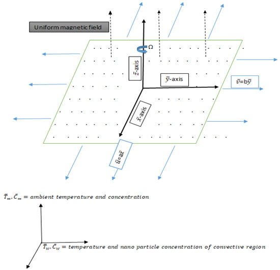
Figure 1. Three-dimensional bi-directional stretching sheet of Powell–Eyring fluid flow.

Cattaneo–Christov theory is incorporated in place of classical [3]. The equations involving heat flux ${\chi }_q$ and mass flux ${\chi }_J$ are given.

$${\chi }_q+{\lambda }_q\left(\frac{\partial {\chi }_q}{\partial \overline{t}}+\overline{V}.\nabla {\chi }_q-{\chi }_q.\nabla \overline{V}+(\nabla .\overline{V}){\chi }_q\right)=-K\nabla \overline{T}$$

(8)

$${\chi }_J+{\lambda }_J\left(\frac{\partial {\chi }_J}{\partial \overline{t}}+\overline{V}.\nabla {\chi }_J-{\chi }_J.\nabla \overline{V}+(\nabla .\overline{V}){\chi }_J\right)=-{\overline{D}}_B\nabla \overline{C}$$

(9)

where ${\lambda }_q$ is the thermal relaxation time and ${\lambda }_J$ is the concentration relaxation time. To proceed further, we use the Rosseland approximation for the radiative heat flux $q_r$.

$${\overline{q}}_r=-\frac{4{\sigma }_s}{3K_e}\frac{\partial {\overline{T}}^4}{\partial \overline{z}}$$

(10)

where ${\sigma }_s$ is the Stefan-Boltzmann constant and $K_e$ is the mean absorption coefficient.

Expanding ${\overline{T}}^4$ into Taylor series about ${\overline{T}}_{\infty }$ and neglecting higher order terms

$${\overline{T}}^4=4{\overline{T}}_{\infty }^3\overline{T}-3{\overline{T}}_{\infty }^4.$$

(11)

In accordance with the above supposition, the heat and mass transfer equation will reduce to

$$\begin{array}{l}\overline{u}\frac{\partial \overline{T}}{\partial \overline{x}}+\overline{v}\frac{\partial \overline{T}}{\partial \overline{y}}+\overline{w}\frac{\partial \overline{T}}{\partial \overline{z}}=-{\lambda }_q\left[\begin{array}{l}{\overline{u}}^2\frac{{\partial }^2\overline{T}}{\partial {\overline{x}}^2}+{\overline{v}}^2\frac{{\partial }^2\overline{T}}{\partial {\overline{y}}^2}+{\overline{w}}^2\frac{{\partial }^2\overline{T}}{\partial {\overline{z}}^2}+2\overline{u}\overline{v}\frac{{\partial }^2\overline{T}}{\partial \overline{x}\partial \overline{y}}+2\overline{v}\overline{w}\frac{{\partial }^2\overline{T}}{\partial \overline{y}\partial \overline{z}}+2\overline{u}\overline{w}\frac{{\partial }^2\overline{T}}{\partial \overline{x}\partial \overline{z}}+\\ \left(\overline{u}\frac{\partial \overline{u}}{\partial \overline{x}}+\overline{v}\frac{\partial \overline{u}}{\partial \overline{y}}+\overline{w}\frac{\partial \overline{u}}{\partial \overline{z}}\right)\frac{\partial \overline{T}}{\partial \overline{x}}+\left(\overline{u}\frac{\partial \overline{v}}{\partial \overline{x}}+\overline{v}\frac{\partial \overline{v}}{\partial \overline{y}}+\overline{w}\frac{\partial \overline{v}}{\partial \overline{z}}\right)\frac{\partial \overline{T}}{\partial \overline{y}}+\left(\overline{u}\frac{\partial \overline{w}}{\partial \overline{x}}+\overline{v}\frac{\partial \overline{w}}{\partial \overline{y}}+\overline{w}\frac{\partial \overline{w}}{\partial \overline{z}}\right)\frac{\partial \overline{T}}{\partial \overline{z}}\end{array}\right]\\ +{\alpha }_t\frac{{\partial }^2\overline{T}}{\partial {\overline{z}}^2}-\frac{16{\sigma }_s{\overline{T}}_{\infty }^3}{3K_e\rho c_p}\frac{{\partial }^2\overline{T}}{\partial {\overline{z}}^2}+\Lambda \left[{\overline{D}}_B\left(\frac{\partial \overline{C}}{\partial \overline{z}}\frac{\partial \overline{T}}{\partial \overline{z}}\right)+\frac{{\overline{D}}_T}{{\overline{T}}_{\infty }}{\left(\frac{\partial \overline{T}}{\partial \overline{z}}\right)}^2\right],\end{array}$$

(12)

$$\begin{array}{l}\overline{u}\frac{\partial \overline{C}}{\partial \overline{x}}+\overline{v}\frac{\partial \overline{C}}{\partial \overline{y}}+\overline{w}\frac{\partial \overline{C}}{\partial \overline{z}}=-{\lambda }_J\left[\begin{array}{l}{\overline{u}}^2\frac{{\partial }^2\overline{C}}{\partial {\overline{x}}^2}+{\overline{v}}^2\frac{{\partial }^2\overline{C}}{\partial {\overline{y}}^2}+{\overline{w}}^2\frac{{\partial }^2\overline{C}}{\partial {\overline{z}}^2}+2\overline{u}\overline{v}\frac{{\partial }^2\overline{C}}{\partial \overline{x}\partial \overline{y}}+2\overline{v}\overline{w}\frac{{\partial }^2\overline{C}}{\partial \overline{y}\partial \overline{z}}+2\overline{u}\overline{w}\frac{{\partial }^2\overline{C}}{\partial \overline{x}\partial \overline{z}}+\\ \left(\overline{u}\frac{\partial \overline{u}}{\partial \overline{x}}+\overline{v}\frac{\partial \overline{u}}{\partial \overline{y}}+\overline{w}\frac{\partial \overline{u}}{\partial \overline{z}}\right)\frac{\partial \overline{C}}{\partial \overline{x}}+\left(\overline{u}\frac{\partial \overline{v}}{\partial \overline{x}}+\overline{v}\frac{\partial \overline{v}}{\partial \overline{y}}+\overline{w}\frac{\partial \overline{v}}{\partial \overline{z}}\right)\frac{\partial \overline{C}}{\partial \overline{y}}+\left(\overline{u}\frac{\partial \overline{w}}{\partial \overline{x}}+\overline{v}\frac{\partial \overline{w}}{\partial \overline{y}}+\overline{w}\frac{\partial \overline{w}}{\partial \overline{z}}\right)\frac{\partial \overline{C}}{\partial \overline{z}}\end{array}\right]\\ +{\overline{D}}_B\frac{{\partial }^2\overline{C}}{\partial {\overline{z}}^2}+\frac{{\overline{D}}_T}{{\overline{T}}_{\infty }}\left(\frac{{\partial }^2\overline{T}}{\partial {\overline{z}}^2}\right)-Q(\overline{C}-{\overline{C}}_{\infty }).\end{array}$$

(13)

The boundary conditions associated with the study are

$$\begin{gathered} \begin{array}{l}\overline{u}=\overline{u}(\overline{x})=a\overline{x},\hspace{0.17em}\hspace{0.17em}\hspace{0.17em}\overline{v}=\overline{v}(\overline{y})=b\overline{y},\hspace{0.17em}\hspace{0.17em}\hspace{0.17em}\hspace{0.17em}\overline{w}=0,\hspace{0.17em}\hspace{0.17em}\hspace{0.17em}\hspace{0.17em}\\ -K\frac{\partial \overline{T}}{\partial \overline{z}}=H_1({\overline{T}}_w-\overline{T}),\hspace{0.17em}\hspace{0.17em}\hspace{0.17em}\hspace{0.17em}-{\overline{D}}_B\frac{\partial \overline{C}}{\partial \overline{z}}=H_2({\overline{C}}_w-\overline{C})\hspace{0.17em}at\hspace{0.17em}\overline{z}=0\end{array} \\ \overline{u}\to 0,\hspace{0.17em}\hspace{0.17em}\hspace{0.17em}\hspace{0.17em}\overline{v}\to 0,\hspace{0.17em}\hspace{0.17em}\hspace{0.17em}\hspace{0.17em}\overline{T}\to {\overline{T}}_{\infty },\hspace{0.17em}\hspace{0.17em}\hspace{0.17em}\hspace{0.17em}\overline{C}\to {\overline{C}}_{\infty }\hspace{0.17em}\hspace{0.17em}\hspace{0.17em}\hspace{0.17em}\hspace{0.17em}\hspace{0.17em}\hspace{0.17em}as\hspace{0.17em}\hspace{0.17em}\overline{z}\to \infty . \end{gathered}$$

(14)

Selecting the following similarity transformations

$$\begin{array}{l}\eta =\sqrt{\frac{a}{\upsilon }}\overline{z},\hspace{0.17em}\hspace{0.17em}\hspace{0.17em}\hspace{0.17em}\overline{u}=a\overline{x}{\overline{f}}^{\prime }(\eta ),\hspace{0.17em}\hspace{0.17em}\hspace{0.17em}\hspace{0.17em}\overline{v}=a\overline{y}{\overline{g}}^{\prime }(\eta ),\hspace{0.17em}\hspace{0.17em}\hspace{0.17em}\hspace{0.17em}\overline{w}=-\sqrt{a\upsilon }\left(\overline{f}(\eta )+\overline{g}(\eta )\right),\\ \overline{\theta }(\eta )=\frac{\overline{T}-{\overline{T}}_{\infty }}{{\overline{T}}_w-{\overline{T}}_{\infty }},\hspace{0.17em}\hspace{0.17em}\hspace{0.17em}\hspace{0.17em}\overline{\phi }(\eta )=\frac{\overline{C}-{\overline{C}}_{\infty }}{{\overline{C}}_w-{\overline{C}}_{\infty }}.\end{array}$$

(15)

The nondimensional equations in view of aforesaid conditions can be written as

$$(1+\overline{n}){\overline{f}}^{‴}-\overline{n}{e}_1{({\overline{f}}^{″})}^2{\overline{f}}^{‴}-{\overline{f}}^{\prime }{}^2+(\overline{f}+\overline{g}){\overline{f}}^{″}+2\gamma \Omega {\overline{g}}^{\prime }-M{\overline{f}}^{\prime }=0,$$

(16)

$$(1+\overline{n}){\overline{g}}^{‴}-\overline{n}{e}_2{({\overline{g}}^{″})}^2{\overline{g}}^{‴}-{\overline{g}}^{\prime }{}^2+(\overline{f}+\overline{g}){\overline{g}}^{″}+2\frac{\Omega }{\gamma }{\overline{f}}^{\prime }-M{\overline{g}}^{\prime }=0,$$

(17)

$$\left(1+\raisebox{1ex}{$4$}\!\left/ \!\raisebox{-1ex}{$3$}\right.{\overline{N}}_1\right){\overline{\theta }}^{″}+P_r\left({\overline{N}}_b{\overline{\phi }}^{\prime }{\overline{\theta }}^{\prime }+{\overline{N}}_t{\overline{\theta }}^{\prime }{}^2+(\overline{f}+\overline{g}){\overline{\theta }}^{\prime }-{\delta }_t(\overline{f}+\overline{g})({\overline{f}}^{\prime }+{\overline{g}}^{\prime }){\overline{\theta }}^{\prime }+{(\overline{f}+\overline{g})}^2{\overline{\theta }}^{″}\right)=0,$$

(18)

$${\overline{\phi }}^{″}+\left(\raisebox{1ex}{${\overline{N}}_t$}\!\left/ \!\raisebox{-1ex}{${\overline{N}}_b$}\right.\right){\overline{\theta }}^{″}+S_c\left((\overline{f}+\overline{g}){\overline{\phi }}^{\prime }-{\delta }_c(\overline{f}+\overline{g})({\overline{f}}^{\prime }+{\overline{g}}^{\prime }){\overline{\phi }}^{\prime }+{(\overline{f}+\overline{g})}^2{\overline{\phi }}^{″}-\epsilon \overline{\phi }\right)=0.$$

(19)

The corresponding boundary conditions are

$$\begin{gathered} \begin{array}{l}\overline{f}(0)=\overline{g}(0)=0,\hspace{0.17em}\hspace{0.17em}\hspace{0.17em}\hspace{0.17em}{\overline{f}}^{\prime }(0)=1,\hspace{0.17em}\hspace{0.17em}\hspace{0.17em}\hspace{0.17em}{\overline{g}}^{\prime }(0)=A,\hspace{0.17em}\hspace{0.17em}\hspace{0.17em}\\ \hspace{0.17em}{\overline{\theta }}^{\prime }(0)=-{\alpha }_1\left(1-\overline{\theta }(0)\right),\hspace{0.17em}\hspace{0.17em}\hspace{0.17em}\hspace{0.17em}{\overline{\phi }}^{\prime }(0)=-{\alpha }_2\left(1-\overline{\phi }(0)\right)\hspace{0.17em}\hspace{0.17em}\hspace{0.17em}\hspace{0.17em}at\hspace{0.17em}\hspace{0.17em}\eta =0.\end{array} \\ {\overline{f}}^{\prime }(\infty )\to 0,\hspace{0.17em}\hspace{0.17em}\hspace{0.17em}\hspace{0.17em}{\overline{g}}^{\prime }(\infty )\to 0,\hspace{0.17em}\hspace{0.17em}\hspace{0.17em}\hspace{0.17em}\overline{\theta }(\infty )\to 0,\hspace{0.17em}\hspace{0.17em}\hspace{0.17em}\hspace{0.17em}\overline{\phi }(\infty )\to 0\hspace{0.17em}\hspace{0.17em}\hspace{0.17em}\hspace{0.17em}\hspace{0.17em}\hspace{0.17em}\hspace{0.17em}\hspace{0.17em}\hspace{0.17em}as\hspace{0.17em}\hspace{0.17em}\eta \to \infty . \end{gathered}$$

(20)

Here $\overline{n}=\frac{1}{\mu \beta d}, e_1=\frac{a^3{\overline{x}}^2}{2\upsilon d^2}, e_2=\frac{b^3{\overline{y}}^2}{2\upsilon d^2}$ are Eyring-Powell fluid parameters. $A=\frac{b}{a}$ is the stretching ratio parameter. $\Omega =\frac{\mho }{a}$ is the rotation parameter and $\gamma =\overline{\frac{y}{\overline{x}}}$. $M^2=\frac{\sigma {\overline{B}}^2}{a\rho }$ is the magnetic parameter.$ϵ=\frac{Q}{a}$ is chemical reaction parameter. ${\delta }_t=a{\lambda }_q, {\delta }_c=a{\lambda }_j$ denotes the nondimensional thermal and concentration relaxation parameter. ${\overline{N}}_1=\frac{4{\sigma }_s{\overline{T}}_{\infty }^3}{{\alpha }_t{K}_e\rho c_p}$ represent thermal radiation parameter.$P_r=\frac{\upsilon }{{\alpha }_t}$ is Prandtl number. ${\overline{N}}_b=\raisebox{1ex}{$\mathsf{\Lambda }{\overline{D}}_B\left({\overline{C}}_w-{\overline{C}}_{\infty }\right)$}\!\left/ \!\raisebox{-1ex}{$\upsilon $}\right.$ is Brownian motion parameter, ${\overline{N}}_t=\raisebox{1ex}{$\mathsf{\Lambda }{\overline{D}}_T\left({\overline{T}}_w-{\overline{T}}_{\infty }\right)$}\!\left/ \!\raisebox{-1ex}{$\upsilon {\overline{T}}_{\infty }$}\right.$ is thermophoresis parameter. ${\alpha }_1=\frac{H_1}{K}\sqrt{\frac{\upsilon }{a}}$ and ${\alpha }_2=\frac{H_2}{{\overline{D}}_B}\sqrt{\frac{\upsilon }{a}}$ are the heat transfer Biot number and mass transfer Biot number. The engineering components of skin friction coefficient $C_f$, local Nusselt number $N{u}_x$ and the local Sherwood number $S{h}_x$ are represented as follows:

$$C_{f_x}=\frac{{\tau }_{w_x}}{\rho {\overline{u}}_{w_x}^2},\hspace{0.17em}\hspace{0.17em}\hspace{0.17em}\hspace{0.17em}\hspace{0.17em}{C}_{f_Y}=\frac{{\tau }_{w_y}}{\rho {\overline{v}}_{w_y}^2},\hspace{0.17em}\hspace{0.17em}\hspace{0.17em}\hspace{0.17em}\hspace{0.17em}N{u}_x=\frac{\overline{x}{\overline{q}}_w}{K({\overline{T}}_w-{\overline{T}}_{\infty })},\hspace{0.17em}\hspace{0.17em}\hspace{0.17em}\hspace{0.17em}\hspace{0.17em}S{h}_x=\frac{\overline{x}{\overline{h}}_w}{{\overline{D}}_B({\overline{C}}_w-{\overline{C}}_{\infty })},$$

(21)

where ${\overline{q}}_w$ surface heat flux, ${\overline{h}}_w$ surface mass flux, wall shear stress along $\overline{x}$-axis and $\overline{y}$-axis are given by ${\tau }_{w_x}$ and ${\tau }_{w_y}$.

$$\begin{array}{l}{\tau }_{w_x}={\left[\mu \left(\frac{\partial \overline{u}}{\partial \overline{z}}\right)+\frac{1}{\beta d}\left(\frac{\partial \overline{u}}{\partial \overline{z}}\right)-\frac{1}{6\beta d^3}{\left(\frac{\partial \overline{u}}{\partial \overline{z}}\right)}^3\right]}_{\overline{z}=0},\hspace{0.17em}\hspace{0.17em}\hspace{0.17em}\hspace{0.17em}\\ {\tau }_{w_y}={\left[\mu \left(\frac{\partial \overline{v}}{\partial \overline{z}}\right)+\frac{1}{\beta d}\left(\frac{\partial \overline{v}}{\partial \overline{z}}\right)-\frac{1}{6\beta d^3}{\left(\frac{\partial \overline{v}}{\partial \overline{z}}\right)}^3\right]}_{\overline{z}=0},\\ {\overline{h}}_w=-{\overline{D}}_B{\left(\frac{\partial \overline{C}}{\partial \overline{z}}\right)}_{\overline{z}=0},\hspace{0.17em}\hspace{0.17em}\hspace{0.17em}\hspace{0.17em}\hspace{0.17em}{\overline{q}}_w=-K{\left(\frac{\partial \overline{C}}{\partial \overline{z}}\right)}_{\overline{z}=0}\end{array}$$

(22)

By incorporating the above equations, we get

$$\begin{array}{l}{C}_{f_x}\sqrt{R_{e_x}}=(1+\overline{n}){\overline{f}}^{″}(0)-\frac{1}{3}\overline{n}{e}_1{\overline{f}}^{″}{}^3(0),\\ C_{f_y}\sqrt{R_{e_y}}=(1+\overline{n}){\overline{g}}^{″}(0)-\frac{1}{3}\overline{n}{e}_2{\overline{g}}^{″}{}^3(0),\\ \frac{N{u}_x}{\sqrt{R_{e_x}}}=-{\overline{\theta }}^{\prime }(0),\hspace{0.17em}\hspace{0.17em}\hspace{0.17em}\hspace{0.17em}\hspace{0.17em}\frac{S{h}_x}{\sqrt{R_{e_x}}}=-{\overline{\phi }}^{\prime }(0).\end{array}$$

(23)

$R{e}_x, R{e}_y$ are local Reynolds numbers.

3. Method of Solution

Optimal homotopy method [33,34,35,36,37] is adapted to obtain the solutions for the nonlinear Equations (16)–(19) together with boundary conditions. The initial guesses are given as

$$\begin{array}{l}{\overline{f}}_0=1-e^{-\eta },\hspace{0.17em}\hspace{0.17em}{\overline{g}}_0=A(1-e^{-\eta }),\hspace{0.17em}\hspace{0.17em}{\overline{\theta }}_0=\left(\frac{{\alpha }_1}{1+{\alpha }_1}\right)e^{-\eta },\hspace{0.17em}\hspace{0.17em}\hspace{0.17em}{\overline{\phi }}_0=\left(\frac{{\alpha }_2}{1+{\alpha }_2}\right)e^{-\eta }.\\ \end{array}$$

(24)

$${\psi }_{\overline{f}}(\eta )={\overline{f}}^{‴}-{\overline{f}}^{\prime },\hspace{0.17em}\hspace{0.17em}\hspace{0.17em}{\psi }_{\overline{g}}(\eta )={\overline{g}}^{‴}-{\overline{g}}^{\prime },\hspace{0.17em}\hspace{0.17em}\hspace{0.17em}{\psi }_{\overline{\theta }}(\eta )={\overline{\theta }}^{‴}-{\overline{\theta }}^{\prime },\hspace{0.17em}\hspace{0.17em}\hspace{0.17em}{\psi }_{\overline{\phi }}(\eta )={\overline{\phi }}^{‴}-{\overline{\phi }}^{\prime }.$$

(25)

The concept of minimizing the average square residual errors is utilized [33] to find the ideal values of nonzero auxiliary parameters $h_0^f, h_0^g, h_0^{\theta }$, and $h_0^{\phi }$ which are actually responsible for defining the convergence region of homotopy series solutions.

$$E_m^{\overline{f}}=\frac{1}{k+1}{\displaystyle {\sum }_{j=0}^k{\left\{N_{\overline{f}}{\left({\displaystyle {\sum }_{i=0}^m\widehat{f}(\eta ),\hspace{0.17em}\hspace{0.17em}\hspace{0.17em}\hspace{0.17em}{\displaystyle {\sum }_{i=0}^m\widehat{g}(\eta ),\hspace{0.17em}\hspace{0.17em}\hspace{0.17em}\hspace{0.17em}\hspace{0.17em}}{\displaystyle {\sum }_{i=0}^m\widehat{\theta }(\eta ),\hspace{0.17em}\hspace{0.17em}\hspace{0.17em}\hspace{0.17em}\hspace{0.17em}}{\displaystyle {\sum }_{i=0}^m\widehat{\phi }(\eta )\hspace{0.17em}}}\right)}_{\eta =j\delta \eta }\right\}}^{2}d\eta ,}$$

(26)

$$E_m^{\overline{g}}=\frac{1}{k+1}{\displaystyle {\sum }_{j=0}^k{\left\{N_{\overline{g}}{\left({\displaystyle {\sum }_{i=0}^m\widehat{f}(\eta ),\hspace{0.17em}\hspace{0.17em}\hspace{0.17em}\hspace{0.17em}{\displaystyle {\sum }_{i=0}^m\widehat{g}(\eta ),\hspace{0.17em}\hspace{0.17em}\hspace{0.17em}\hspace{0.17em}\hspace{0.17em}}{\displaystyle {\sum }_{i=0}^m\widehat{\theta }(\eta ),\hspace{0.17em}\hspace{0.17em}\hspace{0.17em}\hspace{0.17em}\hspace{0.17em}}{\displaystyle {\sum }_{i=0}^m\widehat{\phi }(\eta )\hspace{0.17em}}}\right)}_{\eta =j\delta \eta }\right\}}^{2}d\eta ,}$$

(27)

$$E_m^{\overline{\theta }}=\frac{1}{k+1}{\displaystyle {\sum }_{j=0}^k{\left\{N_{\overline{\theta }}{\left({\displaystyle {\sum }_{i=0}^m\widehat{f}(\eta ),\hspace{0.17em}\hspace{0.17em}\hspace{0.17em}\hspace{0.17em}{\displaystyle {\sum }_{i=0}^m\widehat{\theta }(\eta ),\hspace{0.17em}\hspace{0.17em}\hspace{0.17em}\hspace{0.17em}\hspace{0.17em}}{\displaystyle {\sum }_{i=0}^m\widehat{\phi }(\eta )\hspace{0.17em}}}\right)}_{\eta =j\delta \eta }\right\}}^{2}d\eta .}$$

(28)

$$E_m^{\overline{\phi }}=\frac{1}{k+1}{\displaystyle {\sum }_{j=0}^k{\left\{N_{\overline{\phi }}{\left({\displaystyle {\sum }_{i=0}^m\widehat{f}(\eta ),\hspace{0.17em}\hspace{0.17em}\hspace{0.17em}\hspace{0.17em}{\displaystyle {\sum }_{i=0}^m\widehat{\theta }(\eta ),\hspace{0.17em}\hspace{0.17em}\hspace{0.17em}\hspace{0.17em}\hspace{0.17em}}{\displaystyle {\sum }_{i=0}^m\widehat{\phi }(\eta )\hspace{0.17em}}}\right)}_{\eta =j\delta \eta }\right\}}^{2}d\eta .}$$

(29)

$$E_m^{\overline{t}}=E_m^{\overline{f}}+E_m^{\overline{g}}+E_m^{\overline{\theta }}+E_m^{\overline{\phi }}$$

(30)

where $E_m^{\overline{t}}$ is the total of the square of residual error, $\delta \eta =0.5,$ $k=20.$ Mathematica package BVPh2.0 has been used to reduce the average residual error. Table 1 is aligned to show the minimized values of the total residual error at various iterations.

Table 1. Optimal convergence control parameter values and total averaged squared residual errors

Order m	${\mathit{h}}_0^{\overline{\mathit{f}}}$	${\mathit{h}}_0^{\overline{\mathit{g}}}$	${\mathit{h}}_0^{\overline{\mathit{\theta }}}$	${\mathit{h}}_0^{\overline{\mathit{\phi }}}$	${\mathit{E}}_{\mathit{m}}^{\overline{\mathit{t}}}$	CPU Time(sec)
2	−0.58	−0.87	−1.90	−1.87	1.89$\times {10 }^{-4}$	14.47
4	−0.53	−1.01	−1.85	−1.84	2.73$\times {10 }^{-5}$	312.73
6	−0.47	−1.08	−1.85	−1.83	1.10$\times {10 }^{-5}$	4452.7
8	−0.43	−1.12	−1.85	−1.84	6.63$\times {10 }^{-6}$	33756.6

In Table 2, the residual errors for $\overline{f}, \overline{g}, \overline{\theta }, \overline{\phi }$ are given at three distinct iterations with the eighth-order optimal convergence control parameters. It is evident that the residual errors are reduced by raising iterations. Therefore, OHAM provides a procedure to select any set of local convergence control parameters to find convergent outcomes.

Table 2. Individual averaged squared residual errors with optimized values at m = 8 from Table 1

Order m	${\mathit{E}}_{\mathit{m}}^{\overline{\mathit{f}}}$	${\mathit{E}}_{\mathit{m}}^{\overline{\mathit{g}}}$	${\mathit{E}}_{\mathit{m}}^{\overline{\mathit{\theta }}}$	${\mathit{E}}_{\mathit{m}}^{\overline{\mathit{\phi }}}$	CPU Time(sec)
4	1.21$\times {10 }^{-5}$	1.67$\times {10 }^{-5}$	7.46$\times {10 }^{-6}$	6.13$\times {10 }^{-6}$	171.38
8	8.23$\times {10 }^{-8}$	4.53$\times {10 }^{-7}$	3.77$\times {10 }^{-6}$	2.32$\times {10 }^{-6}$	314.38
12	3.91$\times {10 }^{-9}$	4.10$\times {10 }^{-8}$	2.32$\times {10 }^{-6}$	1.07$\times {10 }^{-8}$	506.22

4. Effect of Parameters on Powell–Eyring Fluid Flow

The plots of velocities along $\overline{x}$ and $\overline{y}$ direction with coordinate $\eta$ are executed for the important parameters involved in the flow.

Figure 2 and Figure 3 depict the decrease in velocity along both directions as the rotation in the flow increases. Velocity along $\overline{y}$-direction is diminuting more compared to $\overline{x}$-direction, this may be because of the retarding force which has more impact along $\overline{y}$-direction. Figure 4 and Figure 5 narrates the behavior of Powell-Eyring fluid parameter $\overline{n}$ on the velocities. Velocity ascends by increasing non-Newtonian factors along $\overline{x}$-direction, while along $\overline{y}$-axis it increases near the surface and descends away from surface. Dimensionless velocities along $\overline{x}$ and $\overline{y}$ increase with the increasing ratio $\gamma$, as directed in Figure 6 and Figure 7. One of the most prime parameters to entertain for flow behavior is the magnetic parameter $M.$ Velocity parallel to $\overline{y}$-axis escalates by raising magnetic effects, but the reverse behavior is observed when parallel to $\overline{x}$-axis as bent upon by Figure 8 and Figure 9. In Table 3, the skin friction coefficient on the surface is measured up for various values of $\overline{n}$ and $e_1$. We noted that the local skin friction coefficient along $\overline{x}$-axis is reduced for sufficiently large values of $\overline{n}$, hence the smooth flow along $\overline{x}$-direction and reverse is the behavior of skin friction co-efficient if $e_1$ is raised. Table 4 is given to analyze the skin friction co-efficient in absence of MHD, radiation, and chemical reaction. Skin friction coefficient along $\overline{y}$-direction abates for leading values of $e_2$. In accrual, the skin friction co-efficient exceeds for greater values of $\overline{n}$ ($e_2\le 0)$ and recedes for greater values of $\overline{n}$ ($e_2>0)$ as indicated in Table 5. Table 6 is constructed for the special behavior in the absence of MHD, radiation, and chemical reaction.

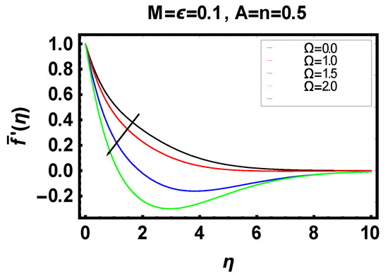
Figure 2. Velocity along $\overline{x}$-direction for variant $\mathsf{\Omega }.$

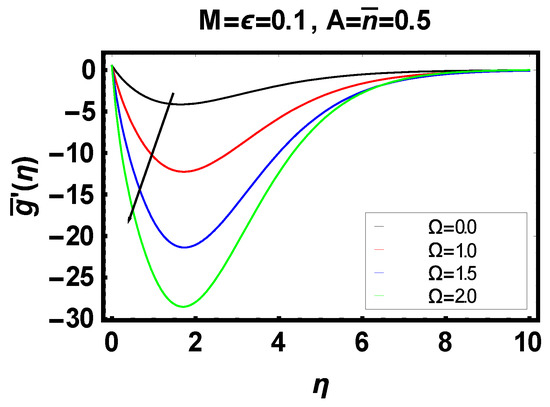
Figure 3. Velocity along $\overline{x}$-direction for variant $\mathsf{\Omega }.$

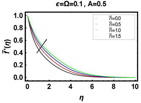
Figure 4. Velocity along $\overline{x}$-direction for variant $\overline{n}.$

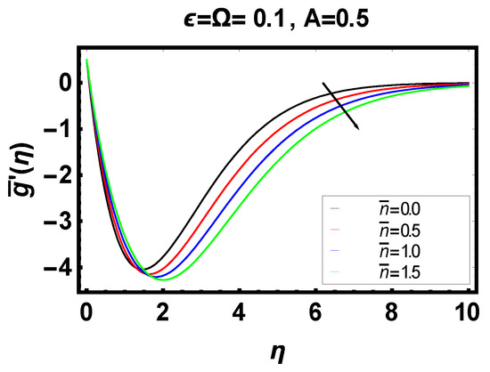
Figure 5. Velocity along $\overline{y}$-direction for variant $\overline{n}.$

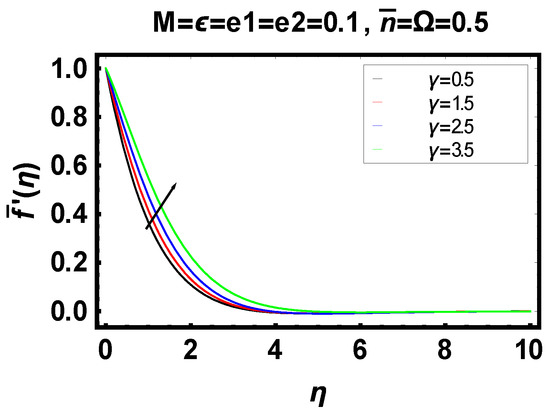
Figure 6. Velocity along $\overline{x}$-direction for variant $\gamma .$

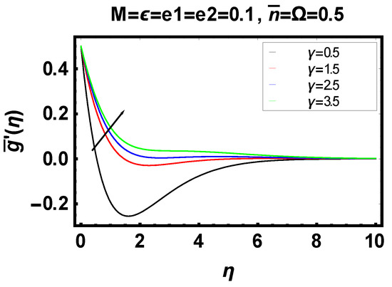
Figure 7. Velocity along $\overline{y}$-direction for variant $\gamma .$

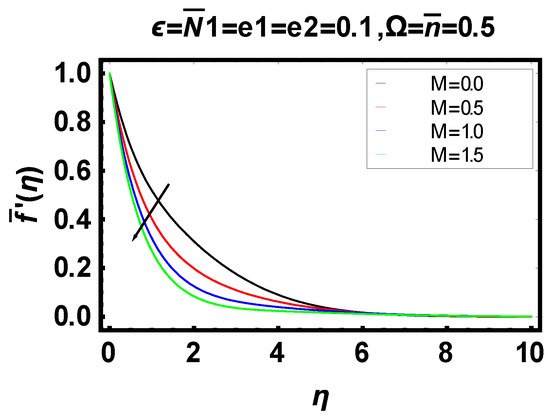
Figure 8. Velocity along $\overline{x}$-direction for variant $M.$

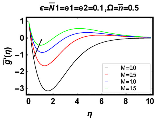
Figure 9. Velocity along $\overline{x}$-direction for variant $M.$

Table 3. Values for $C_{f_x}\sqrt{R{e}_x}$, when ${\mathrm{e}}_2=0.1, \mathsf{\gamma }=0.1, \mathsf{\delta }=0.2,{ \mathsf{\alpha }}_1,{ \mathsf{\alpha }}_2=0.1, \mathrm{M}=0.1, \mathsf{\Omega }=0.5,{ \mathrm{P}}_{\mathrm{r}}=0.7,{ \mathrm{S}}_{\mathrm{c}}=0.2.$

	$\overline{\mathit{n}}$	0.1	0.2	0.3	0.4	0.5
${\mathit{e}}_1$
0		0.3790	−0.2230	−1.0345	−2.0887	−3.4222
0.1		0.4052	−0.1505	−0.8864	−1.8077	−2.8865
0.2		0.4309	−0.0803	−0.7474	−1.5610	−2.4658
0.3		0.4561	−0.0123	−0.6158	−1.3391	−2.1205
0.4		0.4807	0.0533	−0.4907	−1.1355	−1.8237
0.5		0.5048	0.1168	−0.3714	−0.9456	−1.5578

Table 4. Values for $C_{f_x}\sqrt{R{e}_x}$, when ${ \mathrm{e}}_2=0.1, \mathsf{\gamma }=0.1, \mathsf{\delta }=0.2,{ \mathsf{\alpha }}_1,{ \mathsf{\alpha }}_2=0.1, \mathrm{M}=0, {\overline{\mathrm{N}} }_1=0, \mathsf{\Omega }=0.5,{ \mathrm{P}}_{\mathrm{r}}=0.7,{ \mathrm{S}}_{\mathrm{c}}=0.2.$

	$\overline{\mathit{n}}$	0.1	0.2	0.3	0.4	0.5
${\mathit{e}}_1$
0		−0.2609	−0.9519	−1.8591	−3.0163	−4.4604
0.1		−0.2304	−0.8671	−1.6750	−2.6393	−3.7018
0.2		−0.2004	−0.7862	−1.5090	−2.3293	−3.1479
0.3		−0.1709	−0.7086	−1.3572	−2.0674	−2.7315
0.4		−0.1419	−0.6339	−1.2168	−1.8405	−2.4049
0.5		−0.1134	−0.5620	−1.0854	−1.6381	−2.1353

Table 5. Values for $C_{f_y}\sqrt{R{e}_y}$, when ${\mathrm{e}}_1=0.1, \mathsf{\gamma }=0.1, \mathsf{\delta }=0.2,{ \mathsf{\alpha }}_1,{ \mathsf{\alpha }}_2=0.1, \mathrm{M}=0.1, \mathsf{\Omega }=0.5 ,{ \mathrm{P}}_{\mathrm{r}}=0.7,{ \mathrm{S}}_{\mathrm{c}}=0.2.$

	$\overline{\mathit{n}}$	0.1	0.2	0.3	0.4	0.5
${\mathit{e}}_2$
0		55.0297	62.856	71.3146	80.4476	90.2985
0.1		−360.339	−886.582	−1558.52	−2409.23	−3478.23
0.2		−771.59	−1818.44	−3146.07	−4818.55	−6912.48
0.3		−1178.74	−2732.87	−4691.9	−7148.79	−10214.9
0.4		−1581.82	−3630.03	−6196.52	−9401.23	−13388.0
0.5		−1980.84	−4510.1	−7660.48	−11577.1	−16434.2

Table 6. Values for $C_{f_y}\sqrt{R{e}_y}$, when ${ \mathrm{e}}_1=0.1, \mathsf{\gamma }=0.1, \mathsf{\delta }=0.2,{ \mathsf{\alpha }}_1,{ \mathsf{\alpha }}_2=0.1, \mathrm{M}=0, {\overline{\mathrm{N}}}_1=0, \mathsf{\Omega }=0.5,{ \mathrm{P}}_{\mathrm{r}}=0.7,{ \mathrm{S}}_{\mathrm{c}}=0.2.$

	$\overline{\mathit{n}}$	0.1	0.2	0.3	0.4	0.5
${\mathit{e}}_2$
0		52.6231	60.1821	68.3641	77.211	86.766
0.1		−310.516	−772.798	−1366.53	−2122.21	−3076.35
0.2		−669.87	−1589.57	−2762.36	−4247.19	−6114.77
0.3		−1025.46	−2390.28	−4119.65	−6298.98	−9030.92
0.4		−1377.29	−3175.1	−5438.91	−8278.8	−11827.2
0.5		−1725.4	−3944.16	−6720.67	−10187.9	−14506.0

5. Effects of Parameters on Temperature and Concentration

The plots for temperature with coordinate $\eta$ are executed for the important parameters involved in the heat/mass transfer.

Figure 10 is plotted for the analysis of parameter ${\overline{N}}_1$ on $\overline{\theta }$ and $\overline{\phi }$ fields. It can be seen that the temperature of the fluid positively increases as the radiation parameters vary. Further, Figure 11 shows that the volume fraction boundary layer thickens near the sheet, while the reverse effect is noticed away from the sheet with the rising values of radiation parameter. Temperature profile drops with a raise in the magnetic field strength and the concentration field also decline with booming magnetic parameter as illustrated in Figure 12 and Figure 13. Chemical reactions restrained the thermal and concentration fields (Figure 14 and Figure 15). Figure 16 demonstrates typical $\overline{\theta }$ and $\overline{\phi }$ profiles for diverse heat transfer Biot number ${\alpha }_1$. The bold curves show the temperature profile, while the dotted curves mark the concentration profile. We can see that an increase in Biot number depicts an increase in the heat transfer coefficient which is responsible for an increase in temperature and thermal boundary layer thickness. Low heat transfer rate is seen for smaller values of heat transfer coefficient, when it gradually increases, the fluid becomes hotter and has a high rate of heat transfer. This concrete behavior can be seen from Figure 17, that its the concentration of nano fluid accumulated due to an increase in the mass transfer Biot number ${\alpha }_2$. Thermophoresis parameter increases the temperature and concentration profiles while Brownian motion parameter enhances the temperature profile, while the concentration profile decreases with an increase in Brownian motion parameter as explained in Figure 18 and Figure 19. Scrutinizing Table 7, we can see that the heat transfer and mass transfer are enhanced significantly by strengthening the magnetic effect. The same outcomes can be observed by mounting the radiation parameter, heat and mass transfer Biot numbers.

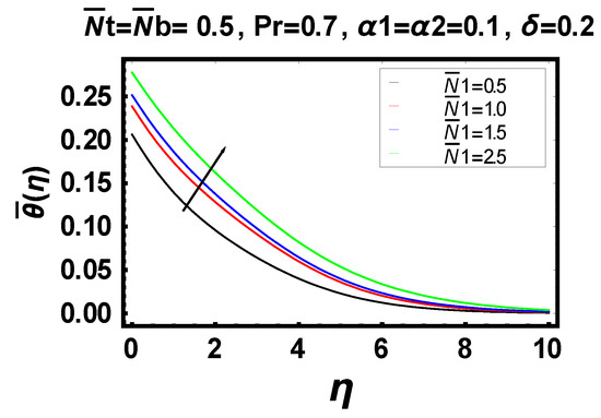
Figure 10. Temperature profile for variant ${\overline{\mathrm{N}}}_1$.

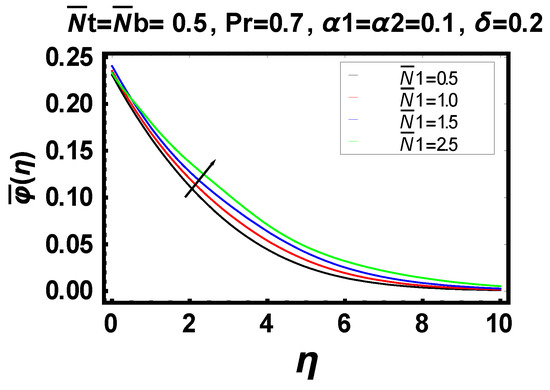
Figure 11. Concentration profile for variant ${\overline{\mathrm{N}}}_1$.

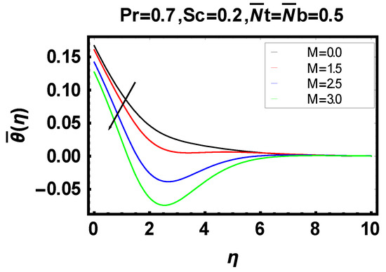
Figure 12. Temperature profile for variant $\mathrm{M}$.

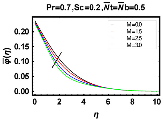
Figure 13. Mass Concentration profile for variant $\mathrm{M}$.

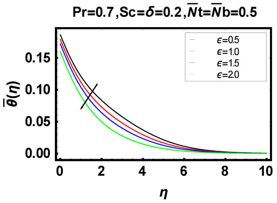
Figure 14. Temperature profile for variant $ϵ$.

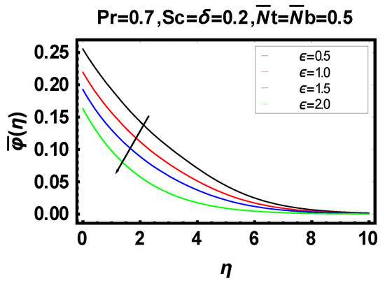
Figure 15. Mass concentration profile for variant $ϵ$.

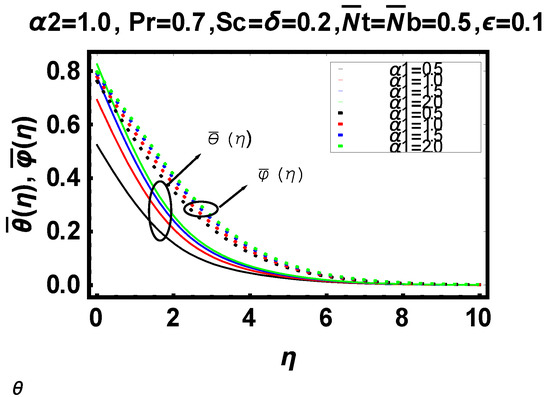
Figure 16. Temperature and concentration profiles for variant ${ \mathsf{\alpha }}_1.$

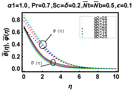
Figure 17. Temperature and concentration profiles for variant ${ \mathsf{\alpha }}_2$.

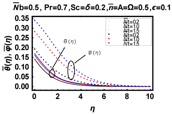
Figure 18. Temperature and concentration profiles for variant ${\overline{\mathrm{N}}}_{\mathrm{t}}$.

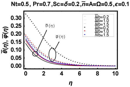
Figure 19. Temperature and concentration profiles for variant ${\overline{\mathrm{N}}}_{\mathrm{b}}$.

Table 7. Computed values of heat transfer rate and mass transfer rate for different values of magnetic parameter $\mathrm{M},$ radiation parameter ${\overline{\mathrm{N}}}_1,$ chemical reaction parameter $ϵ,$ heat transfer biot number ${\mathsf{\alpha }}_1,$ mass transfer biot number ${ \mathsf{\alpha }}_2$.

$\mathbf{M}$	${\overline{\mathrm{N}}}_1$	$\mathit{ϵ}$	${\mathsf{\alpha }}_1$	${\mathsf{\alpha }}_2$	$-{\overline{\mathsf{\theta }}}^{\prime }\left(0\right)$	$-{\overline{\mathsf{\phi }}}^{\prime }\left(0\right)$
0.1	0.1	0	0.1	0.1		0.239077
		0.5				0.249323
		1.0				0.260205
		1.5				0.271679
		2.0				0.283674
0		0.1			0.137712	0.14419
0.5					0.144231	0.145819
1.0					0.151694	0.147705
1.5					0.160144	0.149863
2.0					0.169628	0.152304
0.1			0	0.5	0	0.722521
				1.0	0	1.44597
				2.0	0	2.48147
			1.0	0.5	2.46406	1.59123
				1.0	2.52921	2.86485
				2.0	2.60205	4.53856
			2.0	0.5	4.62906	2.03578
				1.0	4.77689	3.58565
				2.0	4.94091	5.5765
	0		0.1	0.1	0.365409	0.234357
	0.5				0.427331	0.277738
	1.0				0.58768	0.354092
	1.5				0.945752	0.481151
	2.0				1.66287	0.68243

6. Conclusions

For this study of chemically reactive flow of Powell–Eyring nanofluid using non-Fourier’s heat flux and non-Fick’s mass flux theory with radiation, the following developments can be compiled as:

The amplitude of velocity along the $\overline{x}$-direction decreases, while the velocity along the $\overline{y}$-direction increases with the escalating magnetic effect. Temperature rises with the consideration of nanoparticles in the fluid, but the opposite is true for the concentration profile.

Rotational parameter $\Omega$ decreases the velocity boundary layer thickness in the directions.

The Powell–Eyring fluid parameter $\overline{\mathrm{n}}$ has the property of reducing the Nusselt number in both directions.

Heat transfer rate—i.e., the Nusselt number increases as rotation parameter $\Omega$—began to increase. Same response can be seen for increasing magnetic parameter $M$.

Mass transfer rate—i.e., the Sherwood number $Sh$—remains constant for different values of magnetic parameter $M$, while it rises for chemical reaction parameter $ϵ$.

References

- Fourier, J.B.J. Théorie Analytique De La Chaleur; F. Didot: Paris, France, 1822. [Google Scholar]
- Cattaneo, C. Sulla conduzione del calore. Atti Sem. Mat. Fis. Univ. Modena 1948, 3, 83–101. [Google Scholar]
- Christov, C. On frame indifferent formulation of the Maxwell–Cattaneo model of finite-speed heat conduction. Mech. Res Commun. 2009, 36, 481–486. [Google Scholar] [CrossRef]
- Straughan, B. Acoustic waves in a Cattaneo-Christov gas. Phys. Lett. A. 2010, 26, 2667–2669. [Google Scholar] [CrossRef]
- Straughan, B. Thermal convection with the Cattaneo–Christov model. Int. J. Heat Mass Transf. 2010, 53, 95–98. [Google Scholar] [CrossRef]
- Hayat, T.; Farooq, M.; Alsaedi, A.; Al-Solamy, F. Impact of Cattaneo-Christov heat flux in the flow over a stretching sheet with variable thickness. AIP Adv. 2015, 5, 087159. [Google Scholar] [CrossRef]
- Salahuddin, T.; Malik, M.Y.; Hussain, A.; Bilal, S.; Awais, M. Mhd flow of Cattanneo–Christov heat flux model for williamson fluid over a stretching sheet with variable thickness:using numerical approach. J. Magn. Magn. Mater. 2016, 401, 991–997. [Google Scholar] [CrossRef]
- Hayat, T.; Nadeem, S. Flow of 3D Eyring-Powell fluid by utilizing Cattaneo-Christov heat flux model and chemical processes over an exponentially stretching surface. Results Phys. 2018, 8, 397–403. [Google Scholar] [CrossRef]
- Abbasi, F.M. On Cattaneo-Christov heat flux model for Carreau fluid flow over a slendering sheet. Results Phys. 2017, 7, 310–319. [Google Scholar] [CrossRef]
- Abbasi, F.M.; Shehzad, S.A.; Hayat, T.; Alsaedi, A.; Hegazy, A. Influence of Cattaneo-Christov heat flux in flow of an Oldroyd-B fluid with variable thermal conductivity. Int. J. Numer Methods Heat Fluid Flow. 2016, 26, 2271–2282. [Google Scholar] [CrossRef]
- Hayat, T.; Muhammad, T.; Alsaedi, A.; Mustafa, M. A comparative study for flow of viscoelastic fluids with Cattaneo-Christov heat flux. PLoS ONE 2016, 11, e0155185. [Google Scholar] [CrossRef] [Green Version]
- Powell, R.E.; Eyring, E. Mechanism for the Relaxation Theory of Viscosity. Nature 1944, 154, 427–428. [Google Scholar] [CrossRef]
- Hayat, T.; Iqbal, Z.; Qasim, M.; Obaidat, S. Steady flow of an Eyring Powell fluid over a moving surface with convective boundary conditions. Int. J. Heat Mass Transf. 2012, 55, 1817–1822. [Google Scholar] [CrossRef]
- Akbar, N.S.; Nadeem, S. Characteristics of heating scheme and mass transfer on the peristaltic flow for an Eyring–Powell fluid in an endoscope. Int. J. Heat Mass Transf. 2012, 55, 375–383. [Google Scholar] [CrossRef]
- Jalil, M.; Asghar, S. Flow and heat transfer of Powell–Eyring Fluid over a stretching surface: A Lie Group Analysis. J. Fluids Eng. 2013, 135, 121201. [Google Scholar] [CrossRef]
- Malik, M.Y.; Hussain, A.; Nadeem, S. Boundary layer flow of an Eyring-Powell model fluid due to a stretching cylinder with variable viscosity. Sci. Iran. 2013, 20, 313–321. [Google Scholar]
- Nadeem, S.; Saleem, S. Mixed convection flow of Eyring–Powell fluid along a rotating cone. Results Phys. 2014, 4, 54–62. [Google Scholar] [CrossRef] [Green Version]
- Riaz, A.; Ellahi, R.; Sait, M.S. Role of hybrid nanoparticles in thermal performance of peristaltic flow of Eyring-Powell fluid model. J. Therm. Anal. Calorim. 2020. [Google Scholar] [CrossRef]
- Hayat, T.; Makhdoom, S.; Awais, M.; Saleem, S.; Rashidi, M.M. Axisymmetric Powell-Eyring fluid flow with convective boundary condition: Optimal analysis. Appl. Math Mech. 2016, 37, 919–928. [Google Scholar] [CrossRef]
- Ibrahim, W. Three dimensional rotating flow of Powell-Eyring nanofluid with non-Fourier’s heat flux and non-Fick’s mass flux theory. Results Phys. 2018, 8, 569–577. [Google Scholar] [CrossRef]
- Marsch, E.; Tu, C.Y. Intermittency, non-Gaussian statistics and fractal scaling of MHD fluctuations in the solar wind. Nonlin. Process. Geophys. 1997, 4, 101–124. [Google Scholar] [CrossRef] [Green Version]
- Muhammad, Q.; Afridi, M.I.; Wakif, A.; Thoi, T.N.; Hussanan, A. Second Law Analysis of Unsteady MHD Viscous Flow over a Horizontal Stretching Sheet Heated Non-Uniformly in the Presence of Ohmic Heating: Utilization of Gear-Generalized Differential Quadrature Method. Entropy 2019, 21, 240. [Google Scholar] [CrossRef] [Green Version]
- Nadeem, S.; Akhtar, S.; Abbas, N. Heat transfer of Maxwell base fluid flow of nanomaterial with MHD over a vertical moving surface. Alex. Eng. J. 2020, 59, 1847–1856. [Google Scholar] [CrossRef]
- Qasim, M.; Hayat, T.; Obaidat, S. Radiation effect on the mixed convection flow of a viscoelastic fluid along an inclined stretching sheet. Z. Naturforsch. A 2012, 67, 195–202. [Google Scholar] [CrossRef]
- Mehmood, O.U.; Fetecau, C. A note on radiative heat transfer to peristaltic flow of Sisko fluid. Appl. Bionics and Biomech. 2015, 2015. [Google Scholar] [CrossRef] [PubMed] [Green Version]
- Siva, E.P.; Govindarajan, A. Thermal radiation and Soret effect on MHD peristaltic transport through a tapered asymmetric channel with convective boundary conditions. GJPAM 2016, 12, 213–221. [Google Scholar]
- Mallawi, F.O.M.; Bhuvaneswari, M.; Sivasankaran, S.; Eswaramoorthi, S. Impact of double-stratification on convective flow of a non-Newtonian liquid in a Riga plate with Cattaneo-Christov double-flux and thermal radiation. Ain Shams Eng. J. 2021, 12, 969–981. [Google Scholar] [CrossRef]
- Buongiorno, J. Convective transport in nanofluids. ASME J. Heat Transf. 2005, 128, 240–250. [Google Scholar] [CrossRef]
- Kuznetsov, A.V.; Nield, D.A. Natural convective boundary-layer flow of a nanofluid past a vertical plate. Int. J. Therm. Sci. 2010, 49, 243–247. [Google Scholar] [CrossRef]
- Khan, W.A.; Pop, I. Boundary-layer flow of a nanofluid past a stretching sheet. Int. J. Heat Mass Transf. 2010, 53, 2477–2483. [Google Scholar] [CrossRef]
- Nadeem, S.; Haq, R.; Khan, Z.H. Numerical solution of non-newtonian nanofluid flow over a stretching sheet. Appl. Nano Sci. 2014, 4, 625–631. [Google Scholar] [CrossRef] [Green Version]
- Ahmed, Z.; Nadeem, S.; Saleem, S.; Ellahi, R. Numerical study of unsteady flow and heat transfer CNT-based MHD nanofluid with variable viscosity over a permeable shrinking surface. Int. J. Numer. Method H. 2019, 29, 4607–4623. [Google Scholar] [CrossRef]
- Alvi, N.; Latif, T.; Qamar, H.; Asghar, S. Peristalsis of nanofluid with temperature dependent viscosity. J. Comp. Theor. Nano Sci. 2017, 14, 1417–1430. [Google Scholar] [CrossRef]
- Liao, S.J. An optimal homotopy-analysis approach for strongly nonlinear differential equations. Commun. Nonlin. Sci. Num. Sim. 2010, 15, 2003–2016. [Google Scholar] [CrossRef]
- Nadeem, S.; Mehmood, R.; Akbar, N.S. Optimized analytical solution for oblique flow of a Casson-nano fluid with convective boundary conditions. Int. J. Therm. Sci. 2014, 78, 90–100. [Google Scholar] [CrossRef]
- Saleem, S.; Firdous, H.; Nadeem, S.; Khan, A.U. Convective heat and mass transfer in magneto Walter’s B Nanofluid flow induced by a rotating cone. Arab. J. Sci. Eng. 2019, 44, 1515–1523. [Google Scholar] [CrossRef]
- Saleem, S.; Awais, M.; Nadeem, S.; Mustafa, T.; Sandeep, S. Theoretical analysis of upper-convected Maxwell fluid flow with Cattaneo-Christov heat flux model. Chin. J. Phys. 2017, 55, 1615–1625. [Google Scholar] [CrossRef]
- Awais, M.; Saleem, S.; Hayat, T.; Irum, S. Hydromagnetic couple-stress nanofluid flow over a moving convective wall: OHAM analysis. Acta Astronaut. 2016, 129, 271–276. [Google Scholar] [CrossRef]
Publisher’s Note: MDPI stays neutral with regard to jurisdictional claims in published maps and institutional affiliations. |
© 2021 by the authors. Licensee MDPI, Basel, Switzerland. This article is an open access article distributed under the terms and conditions of the Creative Commons Attribution (CC BY) license (https://creativecommons.org/licenses/by/4.0/).