1. Introduction
Grid operators are responsible for providing a safe and reliable energy grid. For this purpose, the electrical grid is reinforced to cope with the increasing integration of renewable energies. One approach of grid reinforcement is the installation of diagnostic systems to reduce the cost of preventive maintenance measures and personnel cost, as well as reducing downtimes of electrical equipment. Such diagnostic systems monitor electrical equipment in a continuous or event-driven manner to detect abnormal or fault conditions [
1]. In recent years, more and more measurement technology has been installed in the electricity grid [
2,
3]. This leads to large normal-condition measurement databases and the sporadic measurement of abnormal conditions. The normal- and abnormal-condition measurements enable the use of supervised machine learning (ML) diagnostic systems. Such diagnostic systems have the potential to automatically learn complex relationships between the conditions of electrical equipment and measurements to classify normal and abnormal conditions. To train ML-based diagnostic systems, large databases are necessary [
4,
5,
6,
7,
8], and the performance of the diagnostic system depends on the quantity and quality of the data [
9,
10,
11,
12,
13]. Electrical equipment often has a small fault rate [
14], leading to only small databases of abnormal conditions for the training of ML models. Therefore, the full potential of ML-based diagnostic systems is not exploited. One approach to cope with this challenge is using data augmentation methods to augment the training data.
Data augmentation is already widely used for image classification. Images are rotated, cropped, or scaled to generate new images and augment the training data [
8]. In signal analysis tasks, the signals are stretched or compressed, and noise is modulated onto the signals [
15]. This signal processing has been shown to increase the performance of ML models but could also result in unrealistic signals. Synthetic data can also be generated using generative models, e.g., based on deep learning methods. These generative models offer the advantage of learning complex and multidimensional distribution functions of features and using this knowledge to generate high-quality synthetic data. They have been proven to increase the performance of ML models in the medical sector [
8,
10,
16] and the diagnostic of mechanical equipment [
15] and electrical equipment [
7] or electrical grids [
17]. Generative Adversarial Networks (GANs) are often used as generative models. GANs consist of two multilayer perceptrons (MLPs). The first MLP is trained to classify data whether they are ‘synthetic data’ or ‘measurements’. The second MLP is trained to generate synthetic data and maximize the probability of misclassification of the first MLP. The training is carried out in an iterative manner [
18]. Some implementations of GANs also work for tabular data [
19,
20,
21,
22]. The training of GANs is hard as the required time for training can be very long and the training can be unstable, depending on the optimization algorithm. Another generative model, Restricted-Boltzmann machines, can also be included in deep belief networks. This model resulted in higher accuracy for the detection of faults in transmission lines compared to state-of-the-art approaches [
23]. Restricted-Boltzmann machines can be hard to train as it is difficult to calculate the energy gradient function.
However, the existing data augmentation techniques are generic techniques and do not add information about the subsequent diagnostic task to the generated, synthetic data. Such information could be provided by computer-implementable, electromechanical models. The electromechanical models contain information about the functional relationship between the measurement variables and the electrical equipment. Integrating such electromechanical models in data augmentation could improve ML-based diagnostic systems further. Improved diagnostic systems could further reduce maintenance effort, reduce the number of trips and inspections of maintenance personnel due to false alarms, and decrease downtimes of electrical equipment. This could potentially lead to savings for the grid operator.
In this paper, we develop a model-based data augmentation using electromechanical models. The aim of the model-based data augmentation is to generate synthetic data and to increase the performance of ML-based diagnostic systems. The model-based data augmentation is showcased for the diagnostic task of detecting an abnormal condition of a secondary distribution transformer. Measurements such as top tank vibration, voltage, and current measurements from the low-voltage side are available for analysis. In the first step of the analysis, the synthetic data generated by the model-based data augmentation are compared to measurements. In the second step, ML-based diagnostic systems are created using model-based data augmentation and are compared with state-of-the-art diagnostic systems.
2. Generation of Synthetic Data and Data Augmentation
Electromechanical models of electrical equipment generate synthetic data. For the variation of the model output to correspond to that of measurements, all variables influencing the model’s output would have to be considered in the electromechanical model. However, electromechanical models typically represent a simplification of the cause–effect relationships so that the variation of the model output does not correspond to that of the measurements. Considering this variation is essential to generate appropriate synthetic normal- and abnormal-condition data. Therefore, the presented model-based data augmentation uses a stochastic approach to sample parameter values of the electromechanical model [
24,
25]. The variation of measurements can thus be mapped appropriately. The generated synthetic data can then be integrated into the training process of ML models.
2.1. Model-Based Data Augmentation
The model-based data augmentation consists of three key parts and uses available normal-condition measurements as input [
25]:
An algorithm to parametrize the electrical model. The algorithm fits the model’s parameter to subsets of the available normal-condition measurements. This results in a parameter set of the electromechanical model for each measurement subset and thus a parameter database.
An algorithm to sample combinations of parameter values from the previously identified parameter database to simulate normal and abnormal conditions.
An electromechanical model to include additional information about the cause–effect relationships of the electrical equipment.
The electromechanical model is parametrized with the sampled parameter values and is simulated to generate synthetic data.
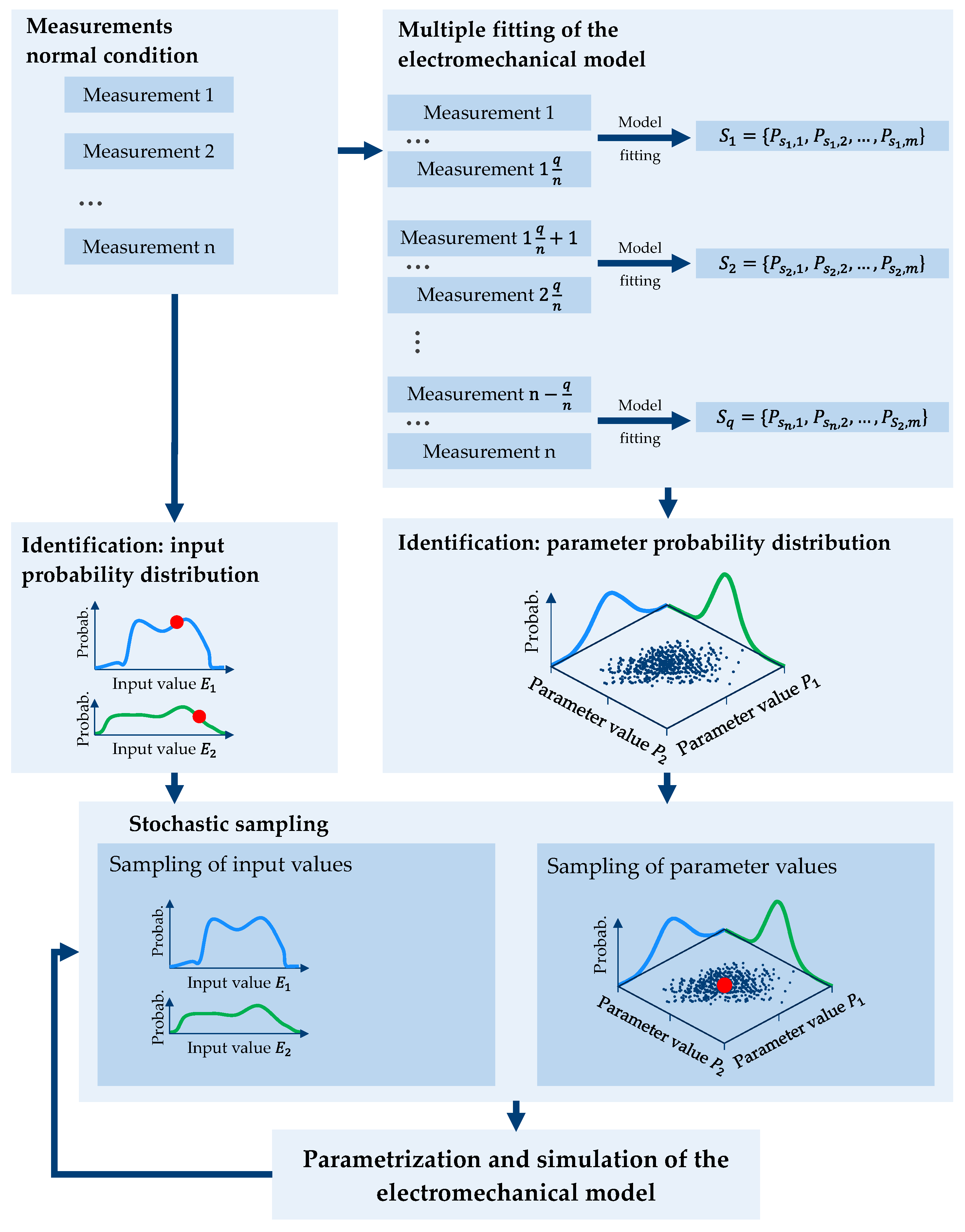
2.1.1. Establishing the Parameter Database and Generating Synthetic Normal-Condition Data
Input and parameter values are necessary for the simulation of an electromechanical model. Both are sampled with a stochastic approach. The process is shown in
Figure 1. In the first step, the probability distributions of the input values are identified from the available normal-condition measurements. In the second step, the
n normal-condition measurements are divided into
q subsets. For each subset, the electromechanical model is fitted to the subset to find the optimal parameter values of the
m parameters of the electromechanical model. This results in
q parameter value sets
S1,…,q. Each parameter value set contains
m parameter values
P1,…,p. These parameter value sets are used to identify a multivariate Gaussian distribution considering the correlation between parameters [
25].
For the generation of synthetic normal-condition data, parameter values and input values are sampled from the corresponding and previously identified probability distributions. The electromechanical model is parametrized with these values and simulated. This results in synthetic normal-condition data with input and corresponding output data. This process is repeated until the desired number of normal-condition data is available.
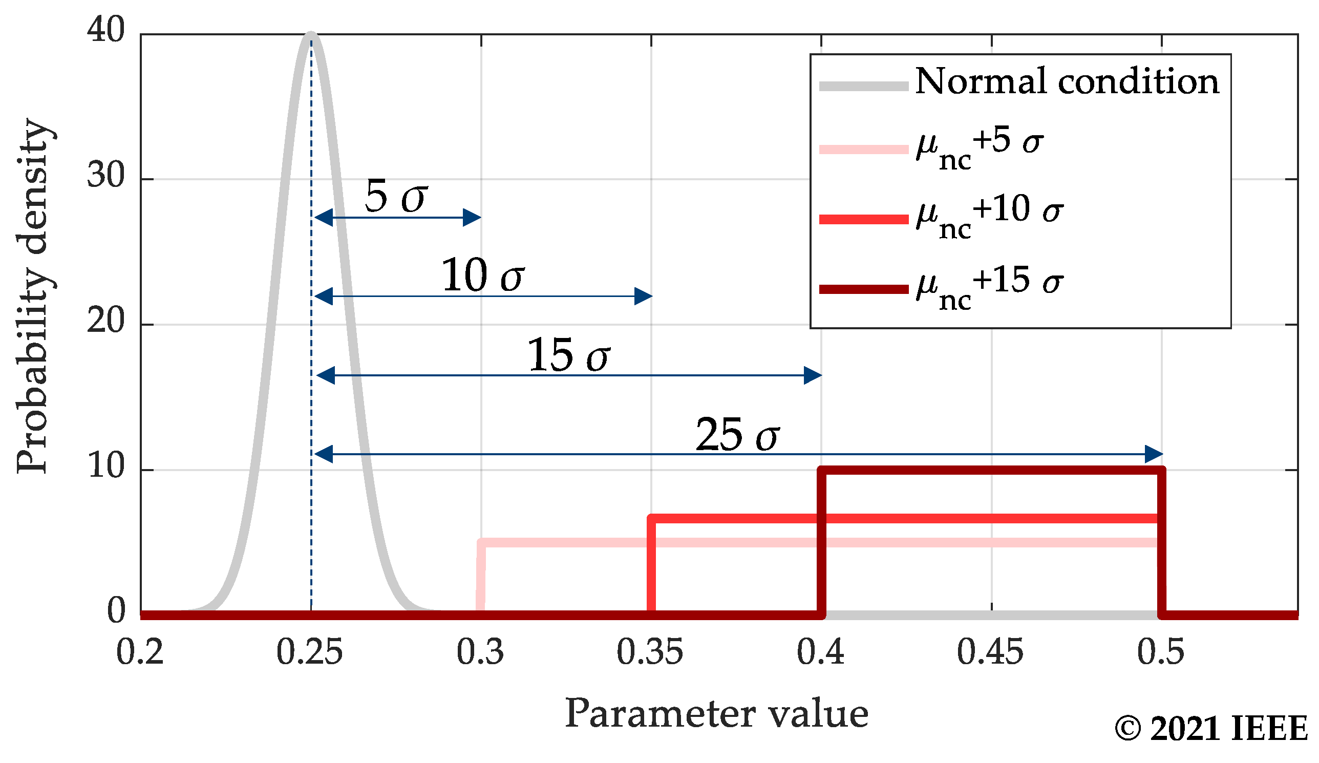
2.1.2. Generating Synthetic Abnormal-Condition Data
For the generation of synthetic abnormal-condition data, parameter values of the electromechanical model are manipulated. Which parameters
Pabnormal are used for this should be selected by domain experts so that the manipulation results in realistic abnormal-condition types. It is not possible to derive the statistically meaningful parameter distributions from measurements as it is often the case that only small databases of abnormal-condition measurements are available. Therefore, the idea behind the abnormal-condition generation is sampling parameter values of the electromechanical model outside the main area of the normal condition’s probability distribution. In this paper, Gaussian distributions are fitted to the parameter values from the database of parameter values (
Section 2.1.1) for each
Pabnormal to represent parameter values for normal conditions. Each Gaussian distribution has a mean value μ
nc and standard deviation σ. To sample parameters outside the main area of these Gaussian distributions, new uniform probability distributions are introduced, representing parameter values for abnormal conditions. In this work, these uniform probability distributions start at
μnc + 5 σ and end at
μnc + 25 σ. This is illustrated in
Figure 2 for different starting points of the probability distribution. Only increasing parameter values are considered because abnormal conditions of transformers lead to an increase of the vibration amplitude [
25].
For the generation of synthetic abnormal-condition data, parameter values and input values are sampled from the multivariate Gaussian distribution from
Section 2.1.1, except for one of the parameters out of
Pabnormal. The value of this parameter is sampled from the introduced uniform probability distribution. The model is parameterized and simulated with the sampled parameter and input values. This results in a data set containing input data and output data representing an abnormal condition. This process can be repeated as often as needed to generate an arbitrary number of synthetic abnormal-condition data.
2.1.3. Electromechanical Model to Simulate Transformer Vibration
The diagnostic task under investigation utilizes vibration, current, and voltage measurements. Thus, an electromechanical model putting these measurement variables into relation is used for the model-based data augmentation. A base model [
26] is modified to consider the individual voltage-dependent magnetostrictions and individual current-dependent electrodynamic forces of the three phases of a distribution transformer. The model calculates the 100 Hz vibration component
A100Hz as a function of the individual effective mean voltages
v and the individual effective mean currents
i across and through phases 1, 2, and 3; see Equation (1). The parameters
α1,
α2, and
α3 and
β1,
β2, and
β3 serve as proportionality factors between vibration and current or voltage as well as damping factors along the propagation path [
26].
The electromechanical model is fitted to measurements to identify values for the parameters α1, α2, and α3 and β1, β2, and β3 using a least-squares method.
Faults such as mechanical deformation or loosening of the winding or core, insulation degradation of the winding [
27,
28], and highly unsymmetrical load can lead to an increased vibration amplitude.
2.2. Integration of Synthetic Data into the Training Process
The synthetic data generated by the model-based data augmentation can be integrated into the training process of ML models using two approaches. The first approach augments the training data with the synthetic data. These augmented training data are used for the training of MLPs. The second approach uses synthetic data as a source domain to train MLPs. These models are then retrained with measurements utilizing transfer learning methods.
2.2.1. Augmenting the Training Data
The un-augmented training data consists of normal- and abnormal-condition measurements. Therefore, the model-based data augmentation can be used to generate and augment normal and abnormal conditions or to only augment abnormal conditions [
29]. Both methods are analyzed in this work.
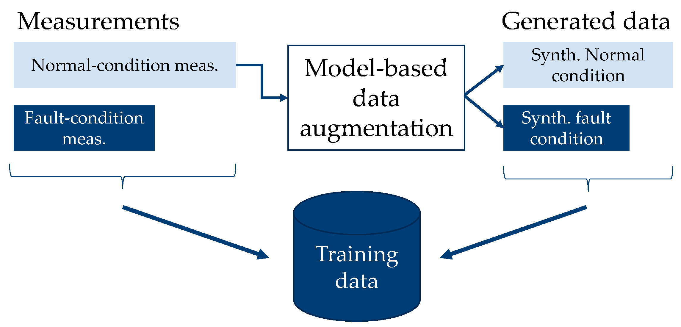
Figure 3 illustrates how synthetic data are generated and the constellation of the training data when they are augmented with the synthetic normal- and abnormal-condition data.
nDA,nc synthetic normal-condition data and
nDA,ac synthetic abnormal-condition data are generated using
nM,nc normal-condition measurements utilizing model-based data augmentation. The ratio
cDA between the number of synthetic data and measurements can be adjusted with Equations (2) and (3). The MLP is trained with the union of the synthetic normal- and abnormal-condition data and the measurements. Such diagnostic systems are denoted by
MDA-NC-AC (for model-based data augmentation: normal condition and abnormal condition).
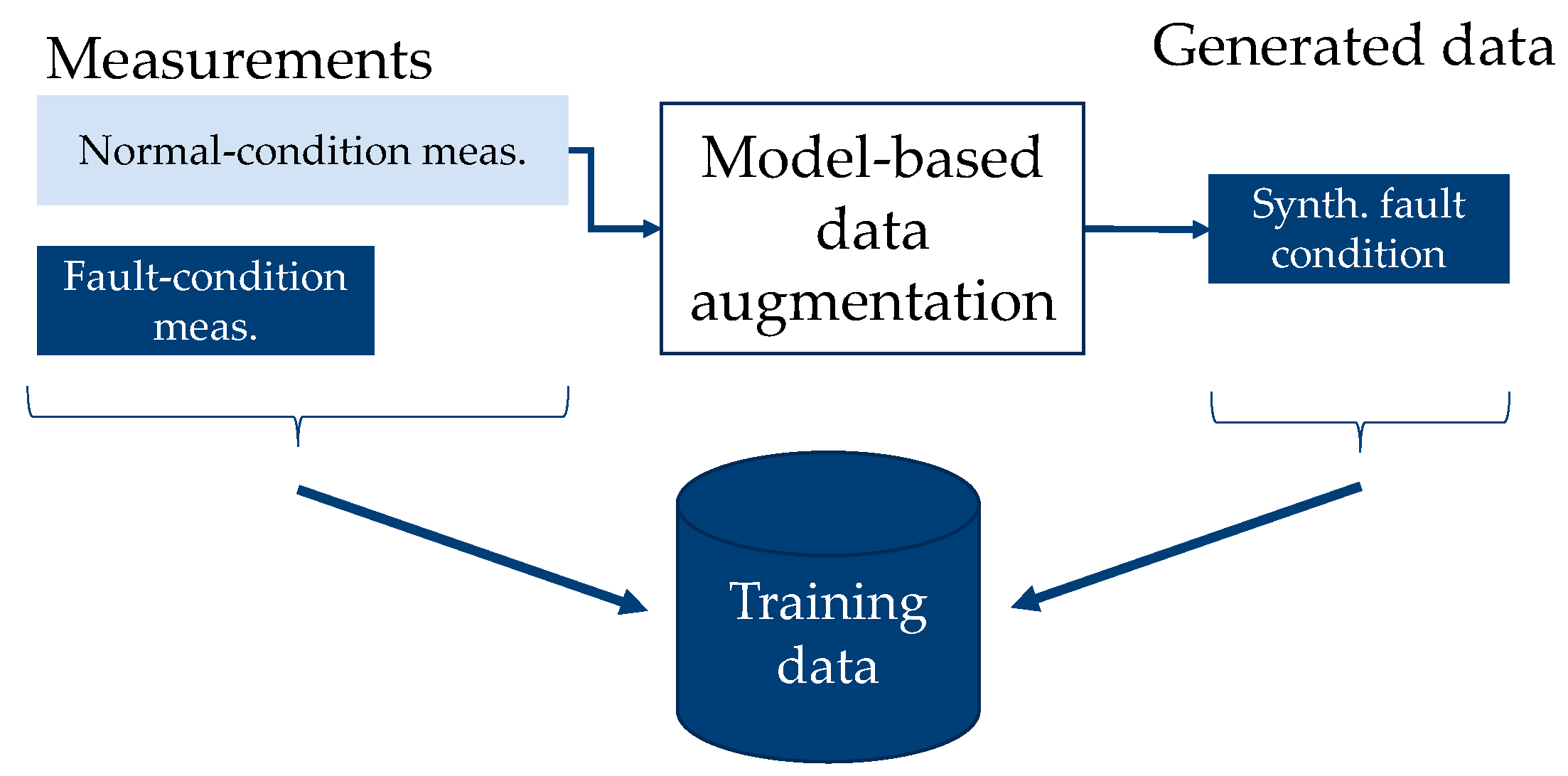
Figure 4 illustrates how synthetic data are generated and the constellation of the training data when it is augmented using only synthetic abnormal-condition data.
nDA,ac synthetic abnormal-condition data are generated using
nM,nc normal-condition measurements utilizing the model-based data augmentation. The union of the synthetic abnormal-condition data and measurements form the training data. The class balance of the training data can be adjusted to a desired class balance
b by limiting the number of synthetic abnormal-condition data added to the training data; see Equation (4). Such diagnostic systems are denoted by
MDA-AC (for model-based data augmentation: abnormal condition).
2.2.2. Generating a Source Domain for Transfer Learning
Transfer learning is normally used to transfer already existing ML models trained on huge databases (source domain) to other tasks or domains. However, such ML models are not available for the diagnostics of electrical equipment. Therefore, a source domain is created with synthetic data generated by the model-based data augmentation using the available normal-condition measurements. The source domain contains synthetic normal- and abnormal condition data. MLPs are trained with this source domain and learn the cause–effect relationships and information provided by the synthetic data during the training process. These MLPs are then transferred to the available normal- and abnormal-condition measurements using transfer learning methods. Retraining the MLPs with measurements offers the potential to reduce the impact of inaccuracies of the electromechanical model or the simulation on the diagnostic system. Generally, knowledge learned in the first training process is preserved in the MLP. The process is shown in
Figure 5. Two methods of transfer learning are considered in this paper: fine-tuning (FT) and feature extraction (FE) [
30].
The first layers of an MLP mostly represent general knowledge, while the back layers contain specific knowledge [
31,
32]. The last layers perform the classification into different classes and do not contain or contain only very little information about the features. The structure of the classification part can be one fully connected layer or multiple layers.
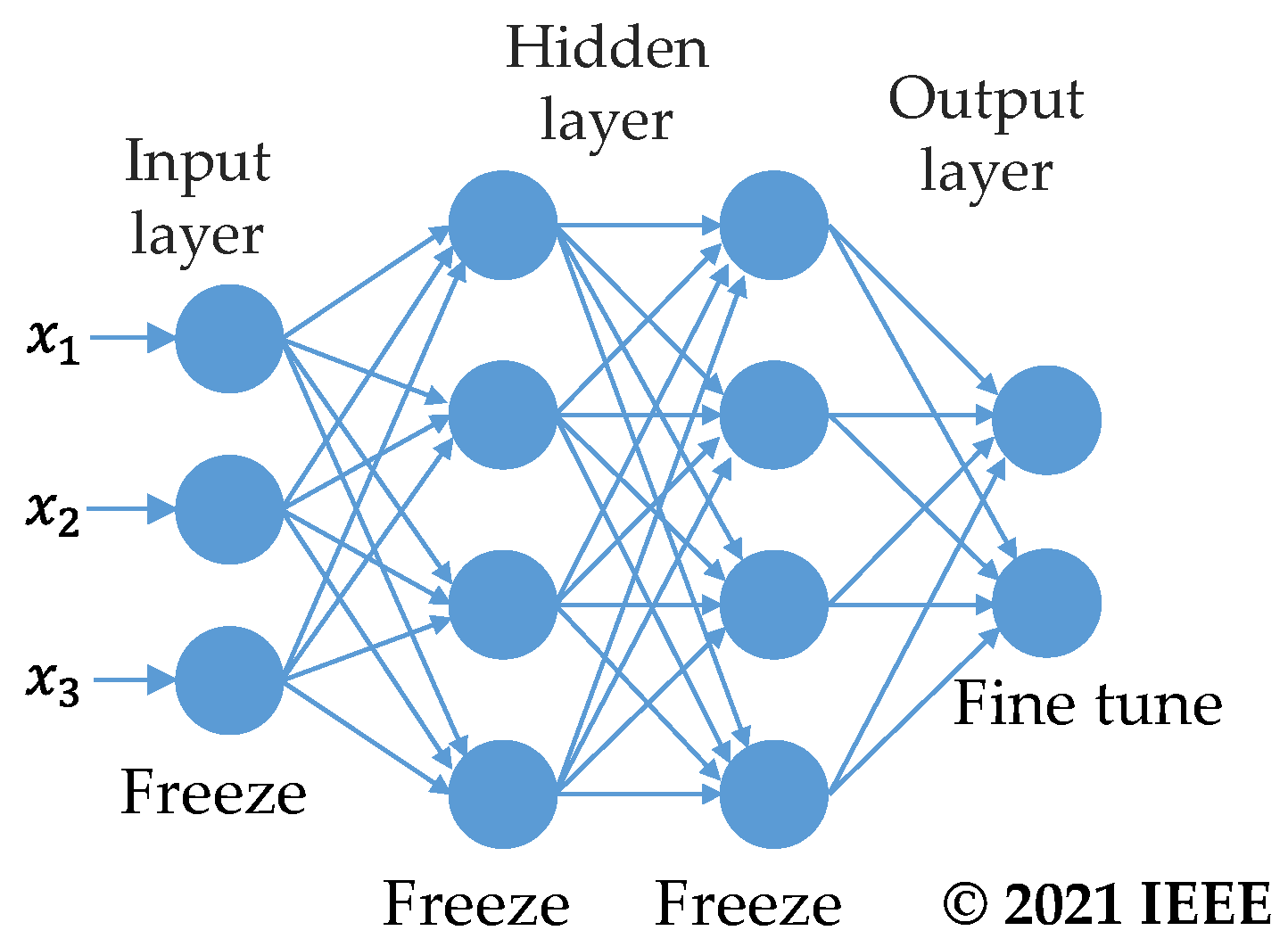
The idea behind fine-tuning is that the structure and knowledge of already trained MLPs are useful for a new domain when adapted. Therefore, this MLP is used as a base model. This model is transferred to the new domain, in the case of this paper to measurements, by retraining the output layer with the measurements (fine-tuning) [
31,
32]. The parameters of the other layers are frozen during this training process, as shown in
Figure 6. Such diagnostic systems are denoted by
MDA-FT.
The second transfer learning method utilized in this paper is feature extraction. The classic use case of feature extraction is transferring an MLP to a new task. This is completed by reusing the part of the MLP where information about features is stored and changing the part of the MLP responsible for the classification, as shown in
Figure 7. The part responsible for the classification is removed from the MLP, and a new classification structure is added. The added structure is retrained with new data while the parameters of the rest of the MLP remain unchanged [
31,
32]. Such diagnostic systems are denoted by
MDA-FE.
In this paper, diagnostic systems utilizing feature extraction are trained with synthetic data and the diagnostic task to classify between normal condition, abnormal condition 1, abnormal condition 2, etc. This MLP is then transferred to measurements with a binary diagnostic task—normal condition or abnormal condition.
3. MLP Structure and Benchmark Diagnostic Systems
To test whether the model-based data augmentation improves the performance of diagnostic systems, diagnostic systems created utilizing the model-based data augmentation are benchmarked with state-of-the-art diagnostic systems. The state-of-the-art diagnostic systems include a model-based diagnostic system, a diagnostic system based on kernel density estimation, an MLP classifier, and an MLP classifier combined with state-of-the-art data augmentation. All MLPs have the same structure.
3.1. Structure of the Multilayer Perceptrons
All diagnostic systems utilizing MLPs use MLPs with identical structures and hyperparameters to achieve comparability between the systems. The chosen structure and hyperparameters do not claim to be the optimal choice for the given diagnostic task.
The MLPs are implemented with
l layers. Each hidden layer has
n nodes. The input layer has seven nodes, one for each normalized feature (100 Hz amplitude of the vibration signal, current phase 1, 2, 3, and voltage phase 1, 2, 3). The output layer contains one node for the binary classification task of
normal condition or
abnormal condition. The number of nodes in the last layer is equal to the number of synthetic abnormal-condition fault types only in the case of the pre-training of MLPs utilizing feature extraction. The activation functions are randomized leaky rectified linear units [
33]. The parameters of the MLPs are optimized with an Adam optimization function [
34], and the MLPs are implemented and trained utilizing PyTorch [
35].
3.2. Model-Based Diagnostic System
Model-based diagnostic systems are widely used as they do not require abnormal-condition measurements [
36,
37,
38,
39,
40,
41]. They use an electromechanical model or an ML model as a predictor for a variable in normal conditions. If a measurement with input data should be analyzed for an abnormal condition, the residuum between the predictor for the given input data and the actual measurement is calculated. If the residuum exceeds a threshold predefined by an expert, an abnormal condition is assumed.
In this paper, a parametrized vibration model from
Section 2.1.3 is used as the predictor for the normal condition. The threshold is set to the threshold that maximizes the diagnostic accuracy for the available measurements to simulate a domain expert setting the optimal threshold. The diagnostic system is illustrated in
Figure 8, where
A denotes the vibration amplitude of the 100 Hz component,
R is the residuum,
v is the voltage,
i is the current, and
α and
β are the parameters of the vibration model. This diagnostic system is denoted by
Res.
3.3. Diagnostic System Based on Kernel Density Estimation
Statistic diagnostic systems also do not require abnormal-condition measurements and are widely used across many domains [
42,
43,
44].
A representative for statistic diagnostic systems, kernel density estimation is used to identify the probability distributions of the input features in normal conditions. Using this probability distribution, the membership of each new measurement to the normal condition can be calculated. An abnormal condition is assumed if the membership undercuts a pre-defined threshold. For this work, the threshold is set to the threshold that maximizes the diagnostic accuracy for the available measurements to simulate a domain expert setting the optimal threshold. This diagnostic system is denoted by KD.
3.4. Multilayer Perceptrons Classifier
Supervised learning classifiers are widely used to classify abnormal conditions [
45,
46,
47,
48,
49]. In this paper, MLPs are trained with training data containing normal- and abnormal-condition measurements. They are denoted by
MLP-Std.
3.5. Multilayer Perceptrons Classifier with State-of-the-Art Data Augmentation
Generative adversarial networks (GANs) are selected as a state-of-the-art data augmentation to benchmark the model-based data augmentation as they are widely used to improve diagnostic systems [
5,
7,
15,
50,
51]. GANs consist of two ML models: a data generator and a data discriminator. The task of the data discriminator is to classify whether data were generated by the data generator or whether the data are measurements. The task of the data generator is to generate realistic synthetic data so that the probability of misclassification by the data discriminator is maximum. These two ML models are trained iteratively [
18].
For this work, the conditional GAN [
22] is slightly modified and used to generate synthetic data. The synthetic data are used to augment the training data in two ways. Either only synthetic abnormal-condition data are generated, or both synthetic normal- and abnormal-condition data are generated to augment the training data, similar to
Section 2.1.3. MLPs are then trained with the augmented training data. Both ways are implemented for this paper and are denoted
GAN-AC (for abnormal condition) and
GAN-NC-AC (for normal condition and abnormal condition).
4. Results and Discussion
The model-based data augmentation is tested for the diagnostic task of detecting an abnormal condition of a secondary distribution transformer. The transformer is a 20° kV/630 kVA transformer with an on-load tap changer on the low-voltage side. The transformer is equipped with sensors to measure the current through and the voltage across each phase on the low-voltage side and a vibration sensor positioned at the tank. The 100 Hz amplitude is extracted from the vibration measurements. The sensors take hourly measurements. In total, measurements of approximately 13 months are available. The absolute load of the transformer for the period under review is shown in
Figure 9. At the beginning of the measurement campaign, the transformer operates in an abnormal condition for approximately 42 days as the on-load tab changer is faulty due to a bad surge arrester in the auxiliary circuit. The transformer is then switched off, the surge arrester is replaced, and the transformer switched on again after 119 more days. Since then, the transformer has operated in normal condition. The measurement campaign resulted in 5614 labeled normal-condition measurements and 1009 labeled abnormal-condition measurements.
The faulty on-load tap changer leads to an unsymmetrical voltage output of the transformer and increased vibration.
Figure 10 shows one of the malfunctioning parameters during the fault: the unsymmetrical voltage. The figure displays the transformer voltage of phase L1, phase L2, and phase L2 for the period under review. During the fault, the voltage of phases L1, L2, and L3 are not symmetrical and have a mean voltage of 233.2 V (L1-N), 230.8 V (L2-N), and 227.8 V (L3-N), respectively. After the repair, the phase imbalance is drastically reduced. The mean voltage is 230.8 V (L1-N), 231.3 V (L2-N), and 231.9 V (L3-N), respectively.
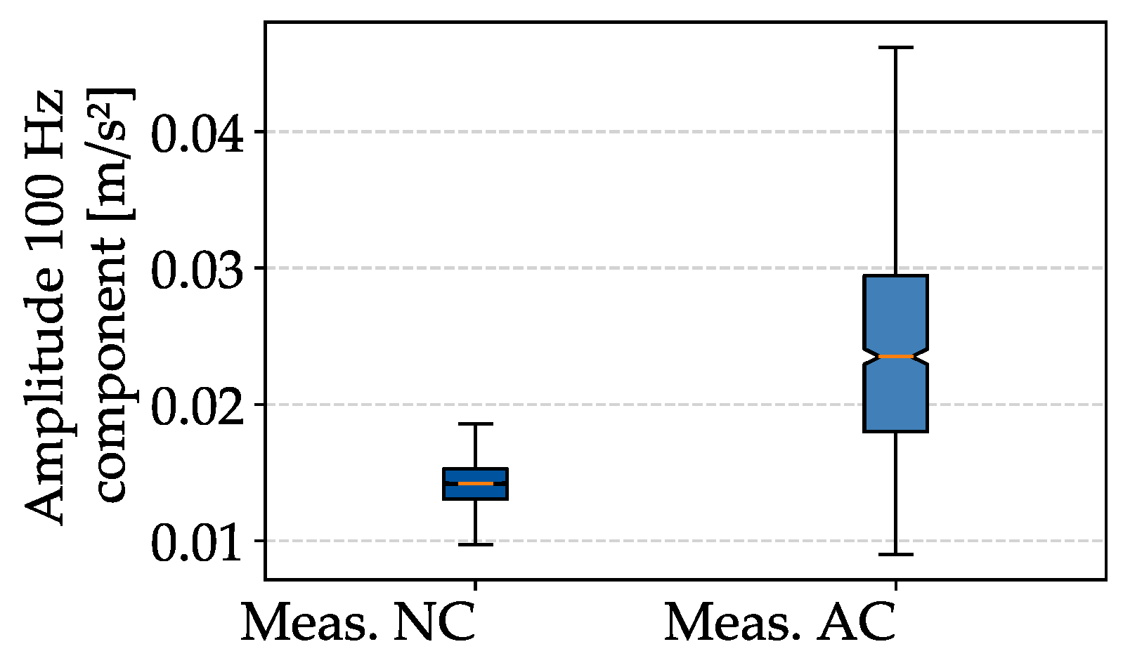
The difference in the vibration amplitude of the normal-condition measurements (meas. NC) and the abnormal-condition measurements (meas. AC) can be seen in the box plots in
Figure 11. The abnormal condition results in higher vibration amplitudes. The distribution of the abnormal-condition measurements has a median of 0.024 m/s
2 and reaches amplitudes up to 0.046 m/s
2, whereas the distribution of the normal-condition measurements has a median of 0.014 m/s
2, and the maximum occurring value is 0.019 m/s
2.
The recorded measurements are used to analyze the model-based data augmentation. First, the synthetic data generated by the model-based data augmentation are compared with the measurements. Then, diagnostic systems utilizing the model-based data augmentation are benchmarked with state-of-the-art diagnostic systems.
4.1. Analysis of Synthetic Normal-Condition Data Generated by the Model-based Data Augmentation
Synthetic data are generated with the model-based data augmentation using all 5614 normal-condition measurements as input data. The results in this section form the foundation of the results shown in
Section 4.2 and are also discussed in [
25].
4.1.1. Synthetic Normal-Condition Data
A total of 10,000 synthetic normal-condition data are generated utilizing the model-based data augmentation. The distribution of the resulting synthetic 100 Hz amplitude (synth. NC) and the normal-condition measurements (meas. NC) is shown as box plots in
Figure 12. The synthetic data’s mean deviates −1.19% from the measurements. The 25%- and 75%-quantile deviates by −8.59% and 5.93% only. This shows that the model-based data augmentation is capable of generating realistic, synthetic, normal-condition data.
4.1.2. Synthetic Abnormal-Condition Data
Synthetic abnormal-condition data are sequentially generated by using the parameters of the electromechanical model
α1,
α2, and
α3 and
β1,
β2, and
β3 as parameters to simulate abnormal conditions. For each of these parameters, 10,000 synthetic abnormal-condition data are generated. The distribution of the synthetic data (synth. NC and Synth. AC) and the measurements, including the 1009 abnormal-condition measurements (meas. AC), are shown in
Figure 13a.
Table 1 shows the percental deviation of characteristic box plot values from the corresponding values of the abnormal-condition measurement. The deviation of the median of the abnormal-condition measurement from the normal-condition measurements is 65.70%. The whiskers of the synthetic abnormal-condition data show a deviation from the median of the abnormal-condition measurements of up to 6475.00%. Even negative vibration amplitudes are generated. With smaller start points and endpoints of the introduced abnormal distribution, realistic abnormal condition data cannot be generated with
β1,
β2, and
β3. This is an indicator that for a realistic abnormal condition simulation with
β, the correlation between the parameters needs to be considered.
Figure 13b shows the distribution of the data without the synthetic abnormal-condition data generated with
β1,
β2, and
β3. The synthetic data generated with
α1,
α2, and
α3 show a distribution similar to the abnormal-condition measurements but is shifted to smaller vibration amplitudes. The median of the synthetic abnormal-condition data deviates from the median of the abnormal-condition measurements by a maximum of −23.82%. The 25% quantile only deviates by up to −17.44% from the 25% quantile of the measurements. The results show that the model-based data augmentation generates realistic synthetic data for independent parameters when properly parametrized.
4.2. Analysis of the Diagnostic Performance of MLPs Created with Model-Based Data Augmentation
Data augmentation methods are often applied when only limited databases are available. Therefore, the model-based data augmentation is analyzed by limiting and successively increasing the number of abnormal-condition measurements in the training data; the number of normal-condition measurements is kept constant. This limitation is carried out to simulate how the ML models would perform if only small abnormal-condition databases were available. Diagnostic systems are created with the limited training data and then tested with test data. The test data contains 80% of the available measurements. Each diagnostic system is trained multiple times for each number of abnormal-condition measurements in the training data with a different constellation of abnormal-condition measurements. The performance on the test data is averaged for each number of abnormal-condition measurements in the training data—similar to cross-validation. The process is illustrated for four abnormal-condition measurements in the training data in
Figure 14.
By successively increasing the number of abnormal-condition measurements in the training data, learning curves can be generated for each diagnostic system. Learning curves plot the performance of a diagnostic system against the number of abnormal-condition measurements in the training data. During the data-limitation process, the class balance between the number of normal-condition measurements and abnormal-condition measurements is kept constant to change only one influence on the performance, the number of abnormal conditions in the training data, at once. The MDA-AC and GAN-AC diagnostic systems allow adding synthetic abnormal-condition data until a pre-defined class balance is met. For the rest of the diagnostic systems, a constant class balance is realized by upsampling the abnormal-condition measurements to a pre-defined value. Upsampling adds data duplicates without adding new information in the form of unseen data to the training data.
The performance of the diagnostic systems is evaluated using accuracy; see Equation (5).
TP are true positive,
TN are true negative,
FP are false positive, and
FN are false negative diagnoses.
Section 4.1.2 shows that the model-based data augmentation does not simulate abnormal conditions with the parameters
β1,
β2, and
β3 properly. Therefore, synthetic abnormal-condition data are simulated with the parameters
α1,
α2, and
α3 in the following. When an abnormal condition is simulated with one of these parameters, the other parameters are sampled from the normal-condition distribution.
4.2.1. Learning Curves of Diagnostic Systems Created with the Model-Based Data Augmentation and State-of-the-Art Diagnostic Systems
In the first step of the analysis, the MLPs of the diagnostic systems have
l = 5 layers, and each hidden layer has
n = 200 neurons.
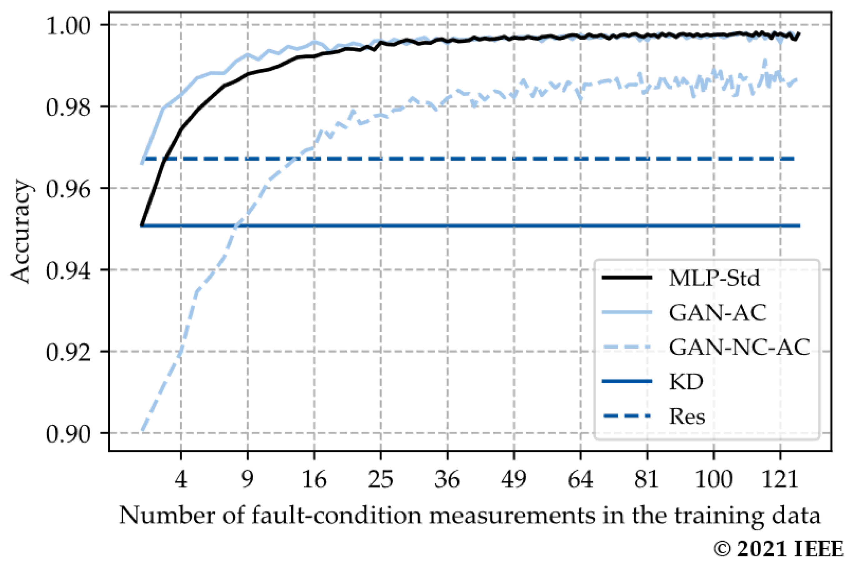
Figure 15 shows the learning curves of the state-of-the-art diagnostic systems. The diagnostic systems
Res and
KD have a constant accuracy (96.6% and 95.0%), as abnormal-condition measurements are not required to create these systems. The accuracy of the MLP-based diagnostic systems
MLP-Std and
GAN-AC is greater than the
Res and
KD diagnostic systems when only three and four abnormal-condition measurements are in the training data. The
GAN-NC-AC diagnostic systems are inferior to the
MLP-Std and
GAN-AC diagnostic systems. The
GAN-AC diagnostic systems are superior to the
MLP-Std systems for <25 abnormal-condition measurements in the training data. The
MLP-Std and
GAN-AC systems converge for a similar accuracy.
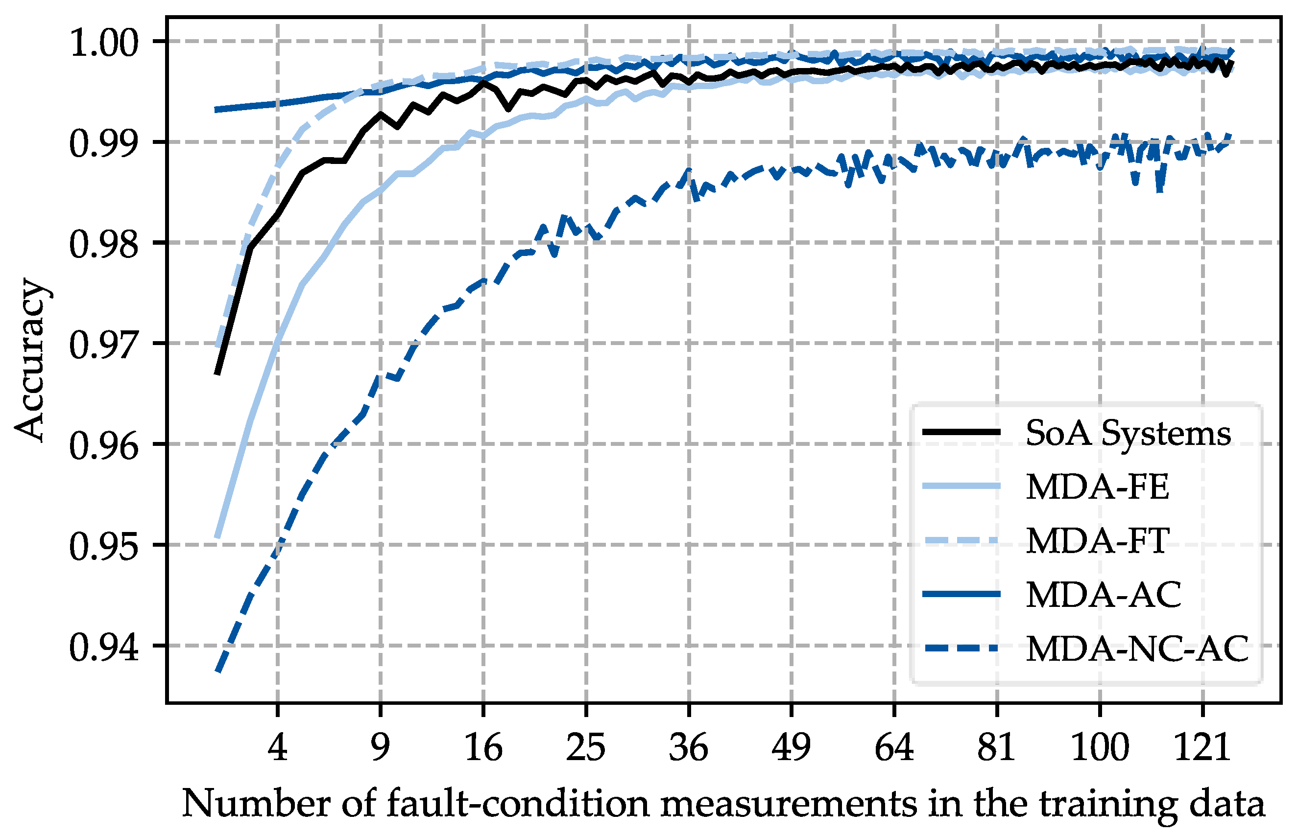
Figure 16 shows the learning curves of the diagnostic systems created with the model-based data augmentation using the approaches presented in
Section 2.2 and the learning curve of the state-of-the-art diagnostic systems. The state-of-the-art diagnostic systems are represented by the maximal envelope curve of the diagnostic systems from
Figure 15 (
SoA systems). For the analysis,
cDA is set to
cDA = 0.5.
The results show that the MDA-NC-AC and MDA-FE diagnostic systems are inferior to the MDA-FT, MDA-AC, and SoA Systems as they have a smaller accuracy for the considered numbers of abnormal-condition measurements. The MDA-FT and MDA-AC diagnostic systems achieve higher diagnostic accuracies than the SoA Systems. The MDA-AC diagnostic systems improve the accuracy, especially for small numbers of abnormal-condition measurements in the training data. The MDA-FT diagnostic systems have, for ≤8 abnormal-condition measurements in the training data, worse accuracy than the MDA-AC diagnostic systems. For >8 abnormal-condition measurements in the training data, the accuracy of the MDA-FT diagnostic systems is, on average, 0.06% greater than the accuracy of the MDA-AC systems.
The results indicate that the model-based data augmentation improves the accuracy of diagnostic systems compared with state-of-the-art diagnostic systems when MDA-FT or MDA-AC systems are used. These diagnostic systems are further analyzed.
4.2.2. Influence of the Number of Layers on Accuracy
In this section, it is analyzed how diagnostic systems utilizing the model-based data augmentation perform compared with state-of-the-art systems for variating numbers of layers. A similar analysis as in
Section 4.2.1 is conducted, but the
MDA-FT,
MDA-AC, and state-of-the-art diagnostic systems are trained with a number of layers variated from
l = 3 layers to
l = 7 layers in steps of 1. The number of neurons per hidden layer is h
l = 200.
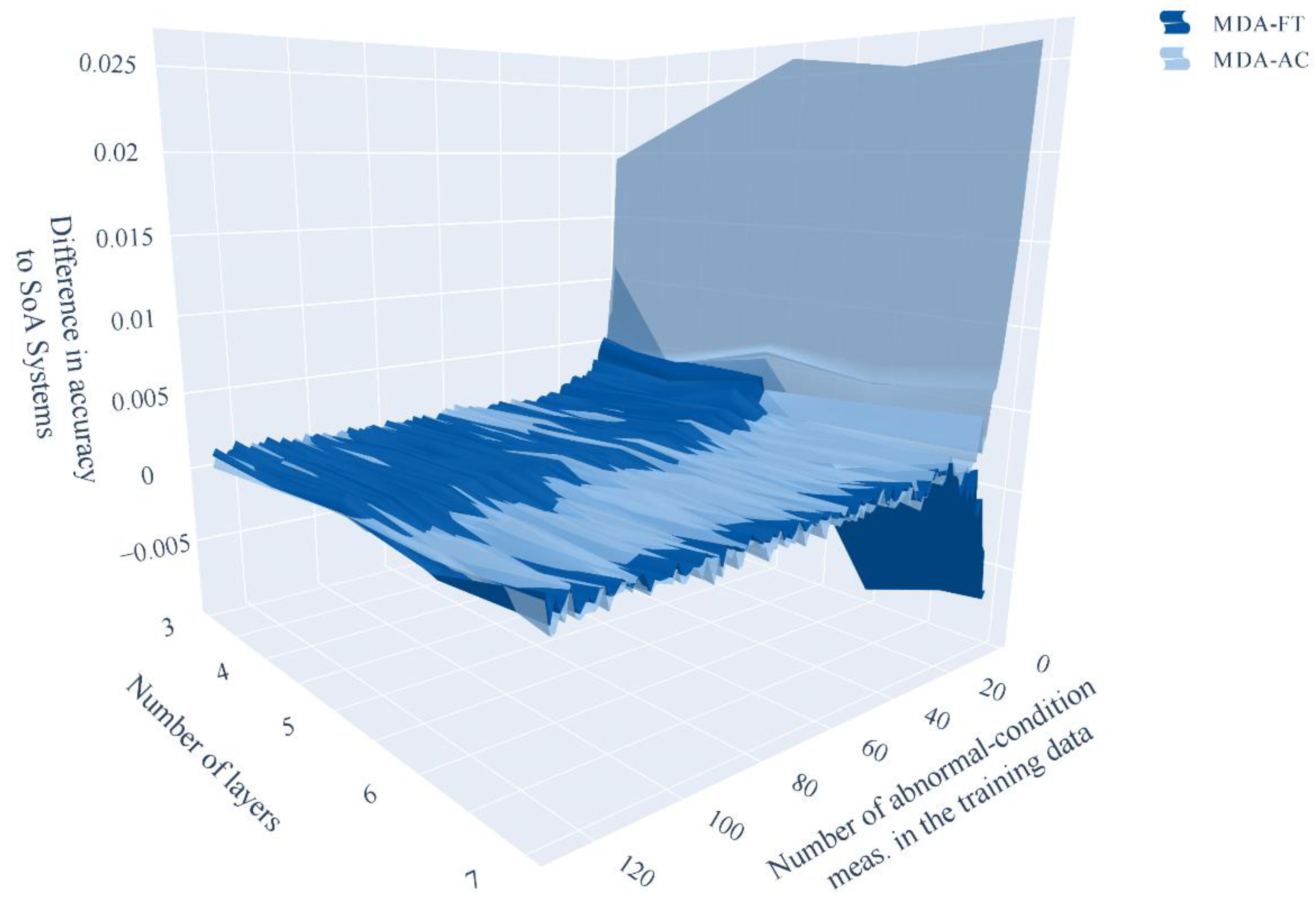
Figure 17 shows the difference in accuracy between
MDA-FT and
MDA-AC diagnostic systems and
SoA Systems with the corresponding number of layers as a function of the number of abnormal-condition measurements in the training data and the number of layers.
Table 2 lists the averaged accuracy difference between the listed diagnostic systems and the
SoA Systems for the analyzed number of layers. The results show that the
MDA-AC and
MDA-FT diagnostic systems achieve greater accuracy than the
SoA Systems for all analyzed number of layers, except the
MDA-FT system with
l = 6 layers. The accuracy of the
MDA-FT system with
l = 6 layers for <17 abnormal-condition measurements in the training data is 0.36% smaller on average than the accuracy of the
SoA Systems. For ≥17 abnormal-condition measurements in the training data, the
MDA-FT system with
l = 6 layers improves the diagnostic performance by 0.11% on average. The accuracy of the
MDA-AC diagnostic systems is, especially for ≤14 abnormal-condition measurements in the training data, larger than the
SoA Systems, on average 0.61%. For >14 abnormal-condition measurements in the training data, the accuracy difference compared to the
SoA Systems is 0.10% on average. The
MDA-FT diagnostic systems outperform the
MDA-AC diagnostic systems for >14 abnormal-condition measurements with an accuracy difference compared to the
SoA Systems of 0.11%.
The results show that the model-based data augmentation combined with MDA-FT and MDA-AC generally improves the accuracy compared to state-of-the-art diagnostic systems for the analyzed number of layers. An improvement of 0.61% results in 53 less misclassifications per year per equipment for hourly measurements. Thus the improvement has a great impact on number of triggered equipment inspections of the equipment owner.
4.2.3. Influence of the Number of Neurons Per Hidden Layer on the Accuracy
In this section, it is analyzed how the diagnostic systems utilizing the model-based data augmentation perform compared with the state-of-the-art systems for variating the numbers of neurons per hidden layer. A similar analysis as in
Section 4.2.1 is conducted, but the
MDA-FT,
MDA-AC, and state-of-the-art diagnostic systems are trained with a number of neurons per hidden layer varied from
n = 50 neurons to
n = 300 neurons in steps of 25. The number of layers is
l = 5.
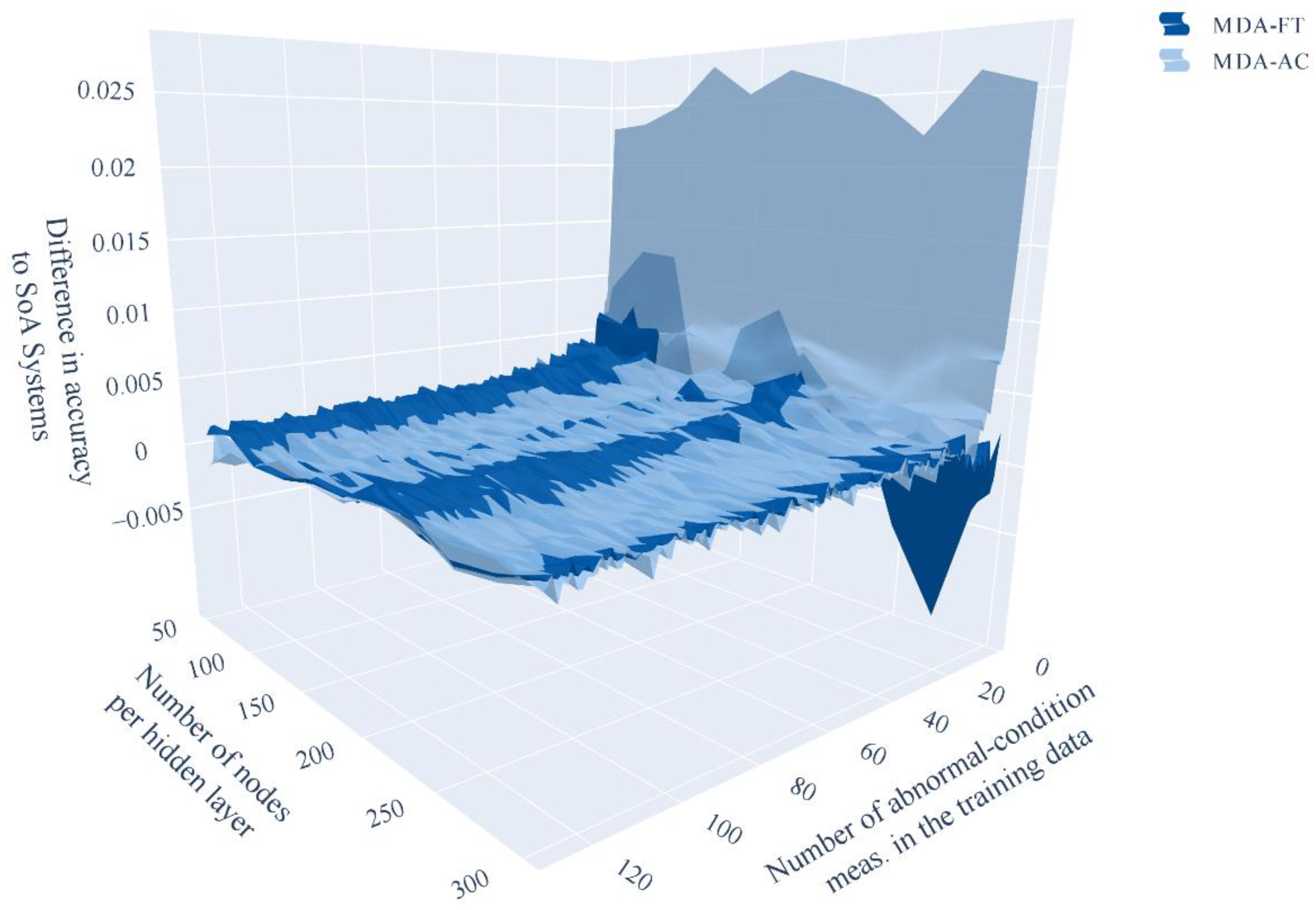
Figure 18 shows the difference in accuracy between
MDA-FT,
MDA-AC diagnostic systems, and
SoA Systems with the corresponding number of neurons per hidden layer as a function of the number of abnormal-condition measurements in the training data and the number of neurons per hidden layer.
Table 3 lists the averaged accuracy difference between the listed diagnostic systems and the
SoA Systems for the analyzed number of neurons per hidden layer. The accuracy of the
MDA-AC and
MDA-FT diagnostic systems are 0.15% and 0.13% higher on average than the
SoA Systems, respectively. Only the
MDA-FT diagnostic systems with
n = 250 neurons result in a smaller averaged accuracy than the
SoA Systems with a difference of −0.01%. For <17 abnormal-condition measurements in the training data, the
MDA-AC diagnostic systems are superior to the
MDA-FT diagnostic systems. The difference in accuracy to the
SoA Systems is 0.21% for
MDA-FT and 0.56% for the
MDA-AC diagnostic systems for <17 abnormal-condition measurements in the training data. For ≥17 normal-condition measurements in the training data, no clear statement can be made as to which of the systems,
MDA-FT or
MDA-AC, is better, as it depends on the number of neurons per hidden layer. The
MDA-AC diagnostic systems have a 0.09% and the
MDA-FT diagnostic systems have a 0.1% higher accuracy than the
SoA Systems averaged over all numbers of neurons per hidden layer.
The results show that the model-based data augmentation combined with MDA-FT and MDA-AC generally improves the accuracy compared to state-of-the-art diagnostic systems for the analyzed number of neurons per hidden layer.
5. Conclusions
Within this paper, we proposed a new model-based data augmentation method to improve the performance of ML-based diagnostic systems by including synthetic data in the training process. The synthetic data are generated utilizing an electromechanical model and a parameter value sampling. Such data are then compared with measurements. The results show that the model-based data augmentation is capable of generating realistic synthetic normal- and abnormal-condition data. Two approaches on how to include these synthetic data into the training process are proposed: augmenting the training data and generating a source domain for transfer learning. Each approach has two types of execution. Diagnostic systems utilizing the model-based data augmentation are trained and compared with state-of-the-art diagnostic systems. The latter includes a model-based diagnostic system, a diagnostic system based on kernel density estimation, an MLP classifier, and an MLP classifier combined with state-of-the-art data augmentation. Including the model-based data augmentation into the training process of ML-based diagnostic systems results in increased accuracy for the MDA-AC and MDA-FT diagnostic systems compared with state-of-the-art diagnostic systems for the analyzed diagnostic task. This holds especially true for the MDA-AC diagnostic systems only if a small number of abnormal-condition measurements are available for the training—this is often the case for power engineering use cases. The average accuracy improvement for <13 abnormal-condition measurements in the training data is 0.68% compared with state-of-the-art diagnostic systems. This corresponds to a reduction of 60 misclassifications per year for hourly measurements of one piece of equipment. For ≥60 abnormal conditions in the training data, the increase in accuracy is smaller. The increase in accuracy compared with state-of-the-art diagnostic systems is, on average, 0.13% for MDA-FT and 0.09% for MDA-AC diagnostic systems. The MDA-AC diagnostic systems should be used only if very few abnormal-condition measurements are available for the training and MDA-FT systems when more abnormal-condition measurements are available for training.
In this paper, the model-based data augmentation is verified for one diagnostic task. The model-based data augmentation should be tested for other diagnostic tasks to identify possible limits.
Author Contributions
Conceptualization, J.N.K.; methodology, J.N.K.; software, J.N.K.; validation, J.N.K.; data curation, J.N.K.; writing—J.N.K.; writing—review and editing, J.N.K., M.A. and A.M.; visualization, J.N.K.; project administration, J.N.K. and M.A.; funding acquisition, J.N.K. and M.A. All authors have read and agreed to the published version of the manuscript.
Funding
This research was funded by the Federal Ministry for Economic Affairs and Energy of Germany in the project MAKSIM—Measurement, information and communication technology to digitalize the asset management of electrical distribution networks (funding codes: 0350035C and 0350035D).
Acknowledgments
Special thanks to the project partners Robert Bosch GmbH and Maschinenfabrik Reinhausen GmbH for developing and installing the measurement systems.
Conflicts of Interest
The funders had no role in the design of the study; in the collection, analyses, or interpretation of data; in the writing of the manuscript, or in the decision to publish the results.
References
- Han, Y.; Song, Y.H. Condition monitoring techniques for electrical equipment-a literature survey. IEEE Trans. Power Deliv. 2003, 18, 4–13. [Google Scholar] [CrossRef]
- Bundesnetzagentur. Monitoringbericht 2017. Available online: https://www.bundesnetzagentur.de/SharedDocs/Mediathek/Monitoringberichte/Monitoringbericht2017.pdf?__blob=publicationFile&v=4 (accessed on 20 June 2021).
- Bundesnetzagentur. Monitoringbericht 2019. Available online: https://www.bundesnetzagentur.de/SharedDocs/Mediathek/Berichte/2019/Monitoringbericht_Energie2019.pdf?__blob=publicationFile&v=6 (accessed on 20 June 2021).
- Dumitrescu, M.; Munteanu, T.; Floricau, D.; Ulmeanu, A.P. A Complex Fault-Tolerant Power System Simulation. In Proceedings of the 2005 2nd International Conference on Electrical and Electronics Engineering, Mexico City, Mexico, 9 September 2005; IEEE: Piscataway, NJ, USA, 2005; pp. 267–272, ISBN 0-7803-9230-2. [Google Scholar]
- Gitzel, R.; Amihai, I.; Garcia Perez, M.S. Towards Robust ML-Algorithms for the Condition Monitoring of Switchgear. In Proceedings of the 2019 First International Conference on Societal Automation (SA), Krakow, Poland, 4–6 September 2019; IEEE: Piscataway, NJ, USA, 2019; pp. 1–4, ISBN 978-1-7281-3345-4. [Google Scholar]
- Meng, Z.; Guo, X.; Pan, Z.; Sun, D.; Liu, S. Data Segmentation and Augmentation Methods Based on Raw Data Using Deep Neural Networks Approach for Rotating Machinery Fault Diagnosis. IEEE Access 2019, 7, 79510–79522. [Google Scholar] [CrossRef]
- Wu, Y.; Lu, C.; Wang, G.; Peng, X.; Liu, T.; Zhao, Y. Partial Discharge Data Augmentation of High Voltage Cables based on the Variable Noise Superposition and Generative Adversarial Network. In Proceedings of the 2018 International Conference on Power System Technology (POWERCON), Guangzhou, China, 8 November 2018; IEEE: Piscataway, NJ, USA, 2018; pp. 3855–3859, ISBN 978-1-5386-6461-2. [Google Scholar]
- Afzal, S.; Maqsood, M.; Nazir, F.; Khan, U.; Aadil, F.; Awan, K.M.; Mehmood, I.; Song, O.-Y. A Data Augmentation-Based Framework to Handle Class Imbalance Problem for Alzheimer’s Stage Detection. IEEE Access 2019, 7, 115528–115539. [Google Scholar] [CrossRef]
- Dobbin, K.K.; Zhao, Y.; Simon, R.M. How large a training set is needed to develop a classifier for microarray data? Clin. Cancer Res. 2008, 14, 108–114. [Google Scholar] [CrossRef] [Green Version]
- Frid-Adar, M.; Klang, E.; Amitai, M.; Goldberger, J.; Greenspan, H. Synthetic data augmentation using GAN for improved liver lesion classification. In Proceedings of the 2018 IEEE 15th International Symposium on Biomedical Imaging (ISBI 2018), Washington, DC, USA, 4–7 April 2018; IEEE: Piscataway, NJ, USA, 2018; pp. 289–293, ISBN 978-1-5386-3636-7. [Google Scholar]
- Kalayeh, H.M.; Landgrebe, D.A. Predicting the required number of training samples. IEEE Trans. Pattern Anal. Mach. Intell. 1983, 5, 664–667. [Google Scholar] [CrossRef] [Green Version]
- Kim, S.-Y. Effects of sample size on robustness and prediction accuracy of a prognostic gene signature. BMC Bioinform. 2009, 10, 147. [Google Scholar] [CrossRef] [Green Version]
- Tam, V.H.; Kabbara, S.; Yeh, R.F.; Leary, R.H. Impact of sample size on the performance of multiple-model pharmacokinetic simulations. Antimicrob. Agents Chemother. 2006, 50, 3950–3952. [Google Scholar] [CrossRef] [Green Version]
- FNN—Forum Netztechnik/Netzbetrieb im VDE. Störungs- und Verfügbarkeitsstatistik: Berichtsjahr 2016; FNN: Berlin, Germany, 2017. [Google Scholar]
- Li, X.; Zhang, W.; Ding, Q.; Sun, J.-Q. Intelligent rotating machinery fault diagnosis based on deep learning using data augmentation. J. Intell. Manuf. 2020, 31, 433–452. [Google Scholar] [CrossRef]
- Sandfort, V.; Yan, K.; Pickhardt, P.J.; Summers, R.M. Data augmentation using generative adversarial networks (CycleGAN) to improve generalizability in CT segmentation tasks. Sci. Rep. 2019, 9, 16884. [Google Scholar] [CrossRef]
- Rahman Fahim, S.; Sarker, S.K.; Muyeen, S.M.; Sheikh, M.R.I.; Das, S.K. Microgrid Fault Detection and Classification: Machine Learning Based Approach, Comparison, and Reviews. Energies 2020, 13, 3460. [Google Scholar] [CrossRef]
- Goodfellow, I.J.; Pouget-Abadie, J.; Mirza, M.; Xu, B.; Warde-Farley, D.; Ozair, S.; Courville, A.; Bengio, Y. Generative Adversarial Networks. arXiv 2014, arXiv:1406.2661. [Google Scholar]
- Choi, E.; Biswal, S.; Malin, B.; Duke, J.; Stewart, W.F.; Sun, J. Generating Multi-label Discrete Patient Records using Generative Adversarial Networks. In Proceedings of the 2nd Machine Learning for Healthcare Conference, Boston, MA, USA, 18–19 August 2017; Doshi-Velez, F., Fackler, J., Kale, D., Ranganath, R., Wallace, B., Wiens, J., Eds.; PMLR: Boston, MA, USA, 2017; pp. 286–305. [Google Scholar]
- Park, N.; Mohammadi, M.; Gorde, K.; Jajodia, S.; Park, H.; Kim, Y. Data synthesis based on generative adversarial networks. Proc. VLDB Endow. 2018, 11, 1071–1083. [Google Scholar] [CrossRef] [Green Version]
- Jordon, J.; Yoon, J.; van der Schaar, M. PATE-GAN: Generating Synthetic Data with Differential Privacy Guarantees. In Proceedings of the 7th International Conference on Learning Representations (ICLR 2019), New Orleans, LA, USA, 6–9 May 2019. [Google Scholar]
- Xu, L.; Skoularidou, M.; Cuesta-Infante, A.; Veeramachaneni, K. Modeling Tabular data using Conditional GAN. In Advances in Neural Information Processing Systems; Wallach, H., Larochelle, H., Beygelzimer, A., Alché-Buc, F., Fox, E., Garnett, R., Eds.; Curran Associates, Inc.: Red Hook, NY, USA, 2019. [Google Scholar]
- Fahim, S.; Sarker, S.; Das, S.; Islam, M.R.; Kouzani, A.; Mahmud, M.A.P. A Probabilistic Generative Model for Fault Analysis of a Transmission Line With SFCL. IEEE Trans. Appl. Supercond. 2021, 31, 1–5. [Google Scholar] [CrossRef]
- Kahlen, J.N.; Mühlbeier, A.; Andres, M.; Rusek, B.; Unger, D.; Kleinekorte, K. Electrical Equipment Analysis and Diagnostics: Methods for Model Parameterization, Fault and Normal Condition Simulation. In Proceedings of the International Conference on Condition Monitoring, Diagnosis and Maintenance, Bucharest, Romania, 9–11 September 2019; pp. 43–52, ISBN 2344-245x. [Google Scholar]
- Kahlen, J.N.; Würde, A.; Andres, M.; Moser, A. Improving Machine Learning Diagnostic Systems with Model-Based Data Augmentation—Part A: Data Generation. In Proceedings of the 2021 IEEE PES Innovative Smart Grid Technologies Europe (ISGT-Europe), Espoo, Finland, 18–21 October 2021; IEEE: Piscataway, NJ, USA, 2021. [Google Scholar]
- Garcia, B.; Burgos, J.C.; Alonso, A. Transformer Tank Vibration Modeling as a Method of Detecting Winding Deformations—Part I: Theoretical Foundation. IEEE Trans. Power Deliv. 2006, 21, 157–163. [Google Scholar] [CrossRef]
- Duan, X.; Zhao, T.; Liu, J.; Zhang, L.; Zou, L. Analysis of Winding Vibration Characteristics of Power Transformers Based on the Finite-Element Method. Energies 2018, 11, 2404. [Google Scholar] [CrossRef] [Green Version]
- Wang, Y. Transformer Vibration and Its Application to Condition Monitoring. Ph.D. Thesis, University of Western Australia, Perth, Australia, 2015. [Google Scholar]
- Kahlen, J.N.; Würde, A.; Andres, M.; Moser, A. Model-based Data Augmentation to Improve the Performance of Machine-Learning Diagnostic Systems. In Proceedings of the 22nd International Symposium on High Voltage Engineering, Xi’an, China, 21–25 November 2021; Németh, B., Ed.; Springer International Publishing: Cham, Switzerland, 2021. in press. [Google Scholar]
- Kahlen, J.N.; Würde, A.; Andres, M.; Moser, A. Improving Machine Learning Diagnostic Systems with Model-Based Data Augmentation—Part B: Application. In Proceedings of the 2021 IEEE PES Innovative Smart Grid Technologies Europe (ISGT-Europe), Espoo, Finland, 18–21 October 2021; IEEE: Piscataway, NJ, USA, 2021. [Google Scholar]
- Sarkar, D.; Bali, R.; Ghosh, T. Hands-On Transfer Learning with Python: Implement Advanced Deep Learning and Neural Network Models Using TensorFlow and Keras; Packt Publishing Ltd.: Birmingham, UK, 2018; ISBN 978-1788831307. [Google Scholar]
- Yang, Q.; Zhang, Y.; Dai, W.; Pan, S.J. Transfer Learning; Cambridge University Press: Cambridge, UK, 2020; ISBN 978-1107016903. [Google Scholar]
- Xu, B.; Wang, N.; Chen, T.; Li, M. Empirical Evaluation of Rectified Activations in Convolutional Network. arXiv 2015, arXiv:1505.00853. [Google Scholar]
- Kingma, D.P.; Ba, J. Adam: A Method for Stochastic Optimization. In Proceedings of the 3rd International Conference on Learning Representations, ICLR 2015, Conference Track Proceedings, San Diego, CA, USA, 7–9 May 2015; Bengio, Y., LeCun, Y., Eds.; ICLR: La Jolla, CA, USA, 2015. [Google Scholar]
- Paszke, A.; Gross, S.; Massa, F.; Lerer, A.; Bradbury, J.; Chanan, G.; Killeen, T.; Lin, Z.; Gimelshein, N.; Antiga, L.; et al. PyTorch: An Imperative Style, High-Perfor-mance Deep Learning Library. In Advances in Neural Information Processing Systems; Wallach, H., Larochelle, H., Beygelzimer, A., Alché-Buc, F., Fox, E., Garnett, R., Eds.; Curran Associates, Inc.: Red Hook, NY, USA, 2019; pp. 8026–8037. [Google Scholar]
- Garcia, B.; Burgos, J.C.; Alonso, A.M. Transformer Tank Vibration Modeling as a Method of Detecting Winding Deformations—Part II: Experimental Verification. IEEE Trans. Power Deliv. 2006, 21, 164–169. [Google Scholar] [CrossRef]
- Svärd, C. Residual Generation Methods for Fault Diagnosis with Automotive Applications; Department of Electrical Engineering, Linköpings Universitet: Linköping, Sweden, 2009; ISBN 978-91-7393-608-8. [Google Scholar]
- Bagheri, M.; Zollanvari, A.; Nezhivenko, S. Transformer Fault Condition Prognosis Using Vibration Signals Over Cloud Environment. IEEE Access 2018, 6, 9862–9874. [Google Scholar] [CrossRef]
- Jalan, A.K.; Mohanty, A.R. Model based fault diagnosis of a rotor–bearing system for misalignment and unbalance under steady-state condition. J. Sound Vib. 2009, 327, 604–622. [Google Scholar] [CrossRef]
- Cho, H.C.; Knowles, J.; Fadali, M.S.; Lee, K.S. Fault Detection and Isolation of Induction Motors Using Recurrent Neural Networks and Dynamic Bayesian Modeling. IEEE Trans. Control Syst. Technol. 2010, 18, 430–437. [Google Scholar] [CrossRef]
- Qian, P.; Ma, X.; Wang, Y. Condition monitoring of wind turbines based on extreme learning machine. In Proceedings of the 21st International Conference on Automation and Computing (ICAC), Glasgow, UK, 11–12 September 2015; IEEE: Piscataway, NJ, USA, 2015; pp. 1–6, ISBN 978-0-9926-8011-4. [Google Scholar]
- Kang, P.; Birtwhistle, D. Condition monitoring of power transformer on-load tap-changers. Part 1: Automatic condition diagnostics. IEE Proc. Gener. Transm. Distrib. 2001, 148, 301. [Google Scholar] [CrossRef]
- Li, H.; Wang, Y.; Liang, X.; He, Y.; Zhao, Y. Nonparametric Kernel Density Estimation Model of Transformer Health Based on Dissolved Gases in Oil. In Proceedings of the 2018 IEEE Electrical Insulation Conference (EIC), San Antonio, TX, USA, 17–20 June 2018; IEEE: Piscataway, NJ, USA, 2018; pp. 236–239, ISBN 978-1-5386-4178-1. [Google Scholar]
- Castellani, F.; Garibaldi, L.; Daga, A.P.; Astolfi, D.; Natili, F. Diagnosis of Faulty Wind Turbine Bearings Using Tower Vibration Measurements. Energies 2020, 13, 1474. [Google Scholar] [CrossRef] [Green Version]
- Huang, X.; Wang, X.; Tian, Y. Research on Transformer Fault Diagnosis Method based on GWO Optimized Hybrid Kernel Extreme Learning Machine. In Proceedings of the 2018 Condition Monitoring and Diagnosis (CMD), Perth, WA, Australia, 23–26 September 2018; IEEE: Piscataway, NJ, USA, 2018; pp. 1–5, ISBN 978-1-5386-4126-2. [Google Scholar]
- Kainaga, S.; Pirker, A.; Schichler, U. Identification of Partial Discharges at DC Voltage using Machine Learning Methods. In Proceedings of the 20th International Symposium on High Voltage Engineering, Buenos Aires, Argentina, 28 August–1 September 2017; Diaz, R., Ed.; Asociación Cooperadora de la Facultad de Ciencias Exactas y Tecnología de la Universidad Nacional de Tucumán: Tucumán, Argentina, 2017. ISBN 978-987-45745-6-5. [Google Scholar]
- Zekveld, M.; Hancke, G.P. Vibration Condition Monitoring using Machine Learning. In Proceedings of the IECON 2018—44th Annual Conference of the IEEE Industrial Electronics Society, Washington, DC, USA, 21–23 October 2018; IEEE: Piscataway, NJ, USA, 2018. [Google Scholar]
- Yuan, F.Q. Critical issues of applying machine learning to condition monitoring for failure diagnosis. In Proceedings of the 2016 IEEE International Conference on Industrial Engineering and Engineering Management (IEEM), Bali, Indonesia, 4–7 December 2016; IEEE: Piscataway, NJ, USA, 2016; pp. 1903–1907, ISBN 978-1-5090-3665-3. [Google Scholar]
- Benmahamed, Y.; Kherif, O.; Teguar, M.; Boubakeur, A.; Ghoneim, S.S.M. Accuracy Improvement of Transformer Faults Diagnostic Based on DGA Data Using SVM-BA Classifier. Energies 2021, 14, 2970. [Google Scholar] [CrossRef]
- Peng, C.; Li, L.; Chen, Q.; Tang, Z.; Gui, W.; He, J. A Fault Diagnosis Method for Rolling Bearings Based on Parameter Transfer Learning under Imbalance Data Sets. Energies 2021, 14, 944. [Google Scholar] [CrossRef]
- Zhong, C.; Yan, K.; Dai, Y.; Jin, N.; Lou, B. Energy Efficiency Solutions for Buildings: Automated Fault Diagnosis of Air Handling Units Using Generative Adversarial Networks. Energies 2019, 12, 527. [Google Scholar] [CrossRef] [Green Version]
| Publisher’s Note: MDPI stays neutral with regard to jurisdictional claims in published maps and institutional affiliations. |
© 2021 by the authors. Licensee MDPI, Basel, Switzerland. This article is an open access article distributed under the terms and conditions of the Creative Commons Attribution (CC BY) license (https://creativecommons.org/licenses/by/4.0/).


