
A Data-Driven Multi-Regime Approach for Predicting Energy Consumption


Abstract
:1. Introduction
1.1. Motivation
1.2. Contribution
2. Related Work
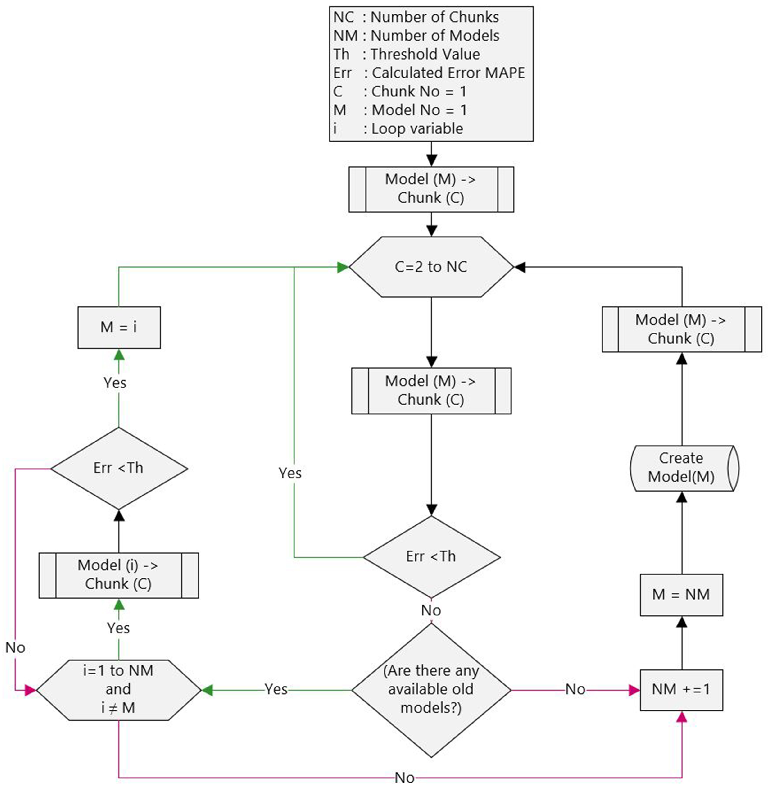
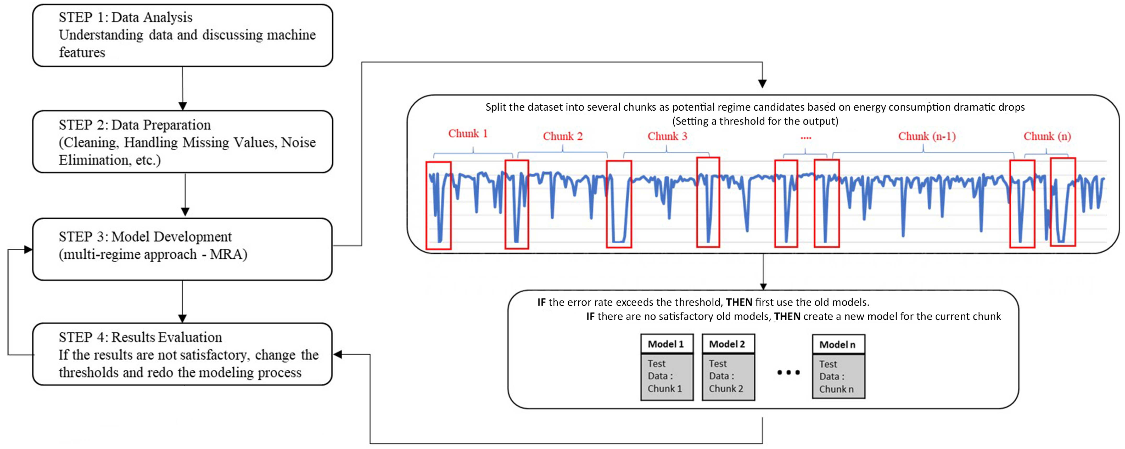
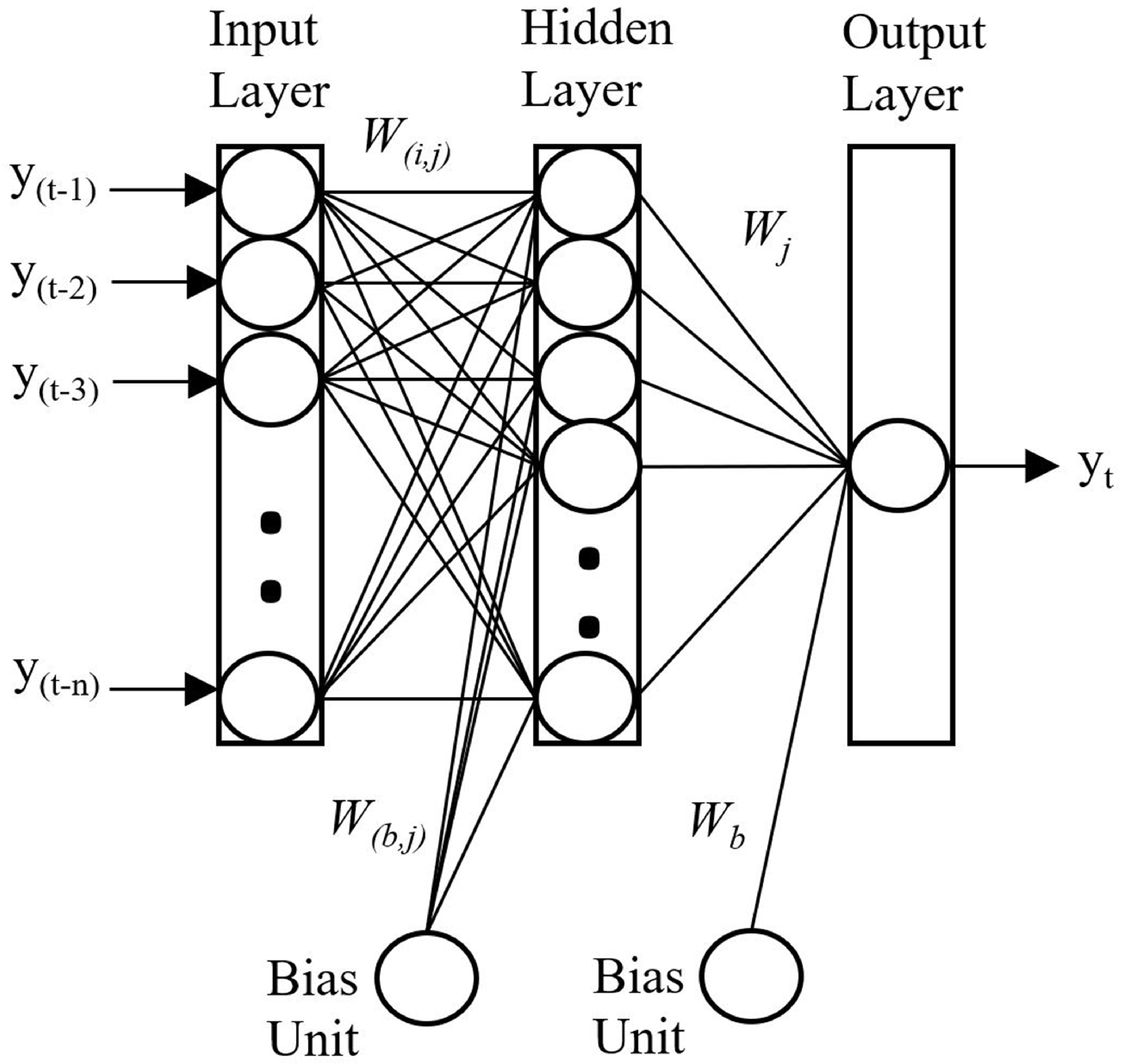
3. Methodology
4. Experiments
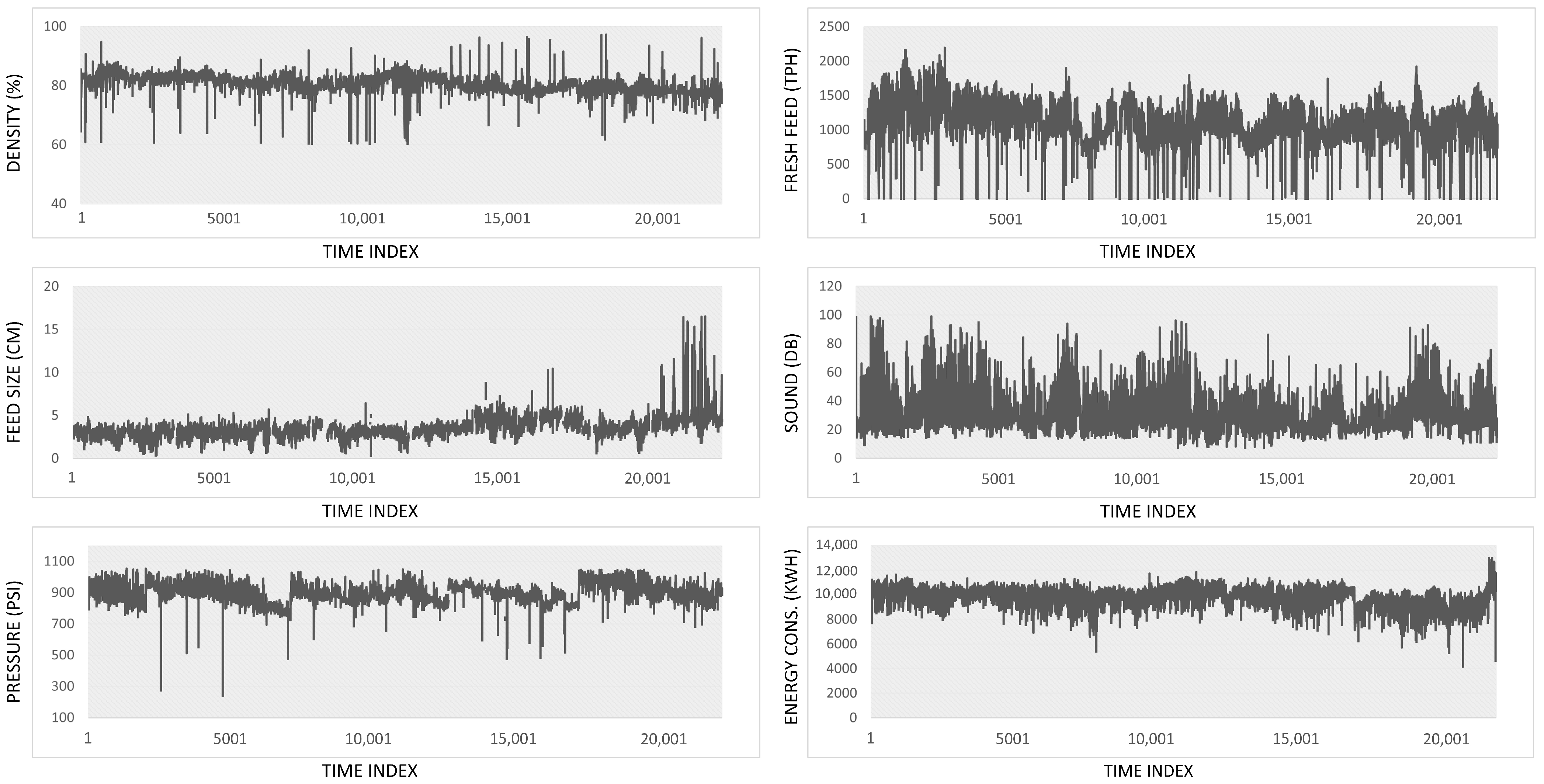
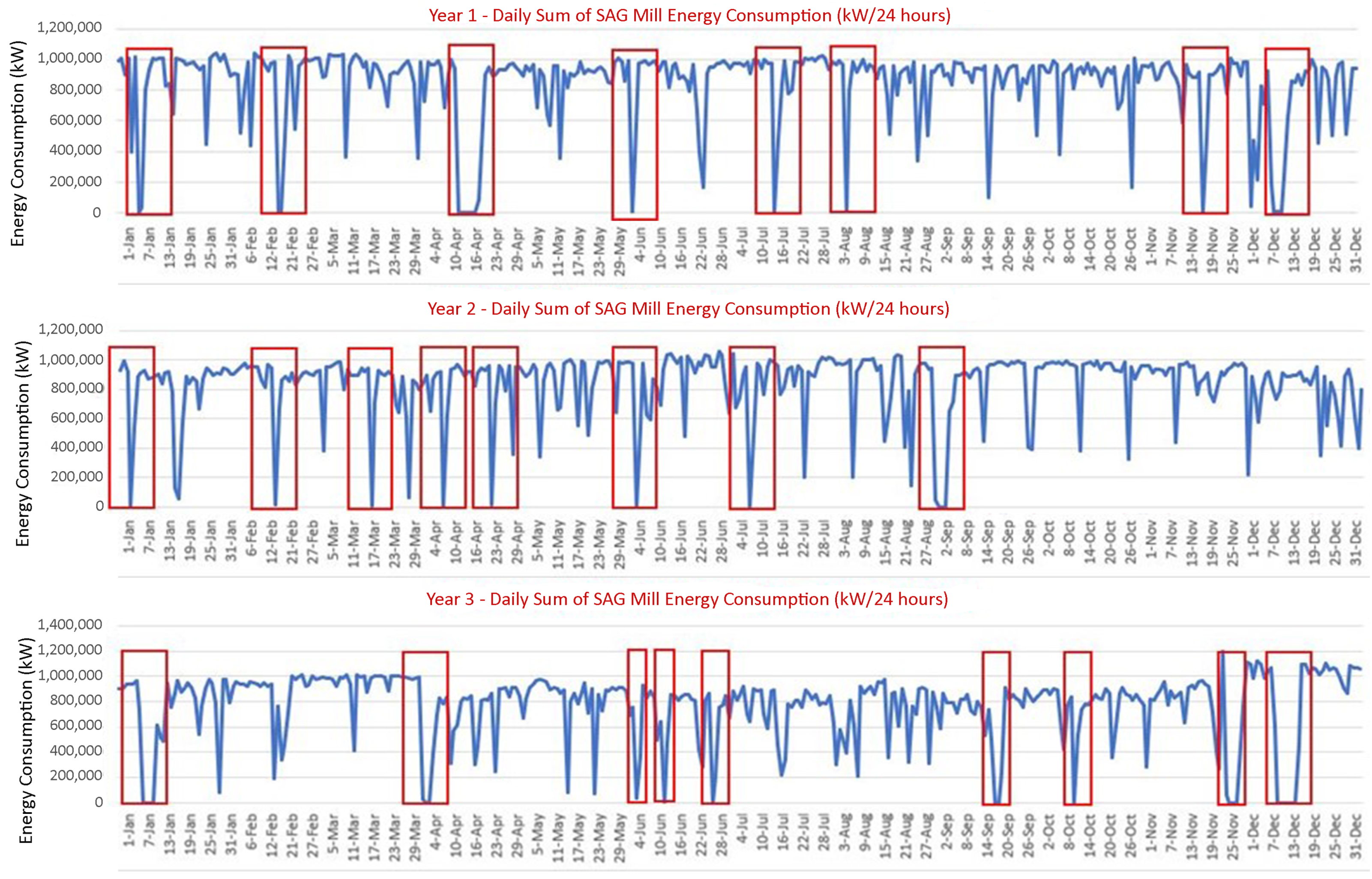
4.1. Dataset
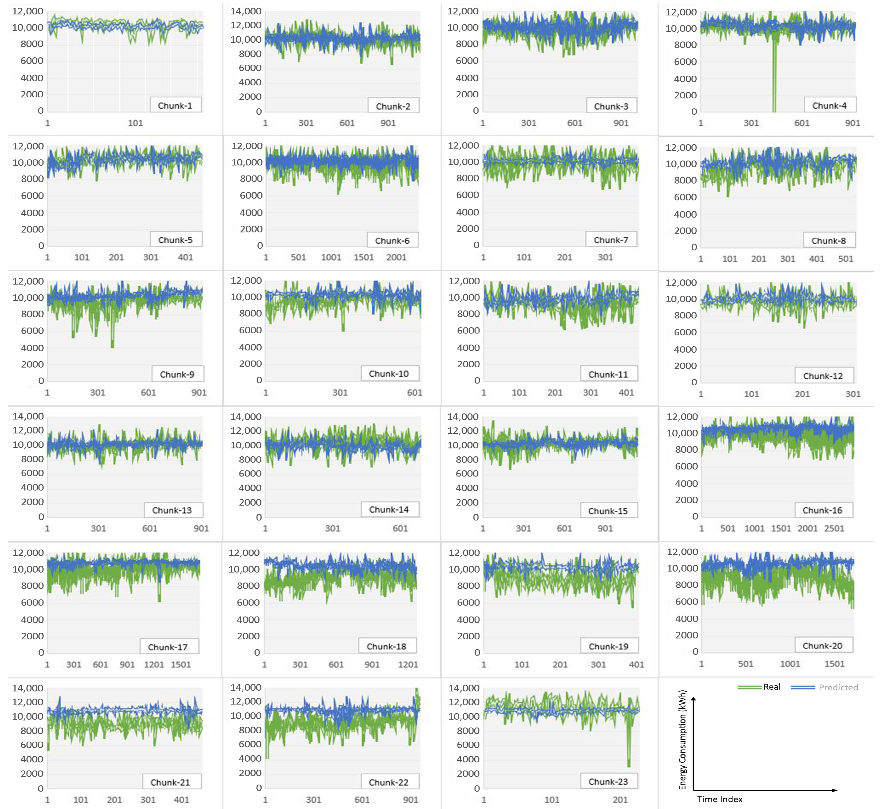
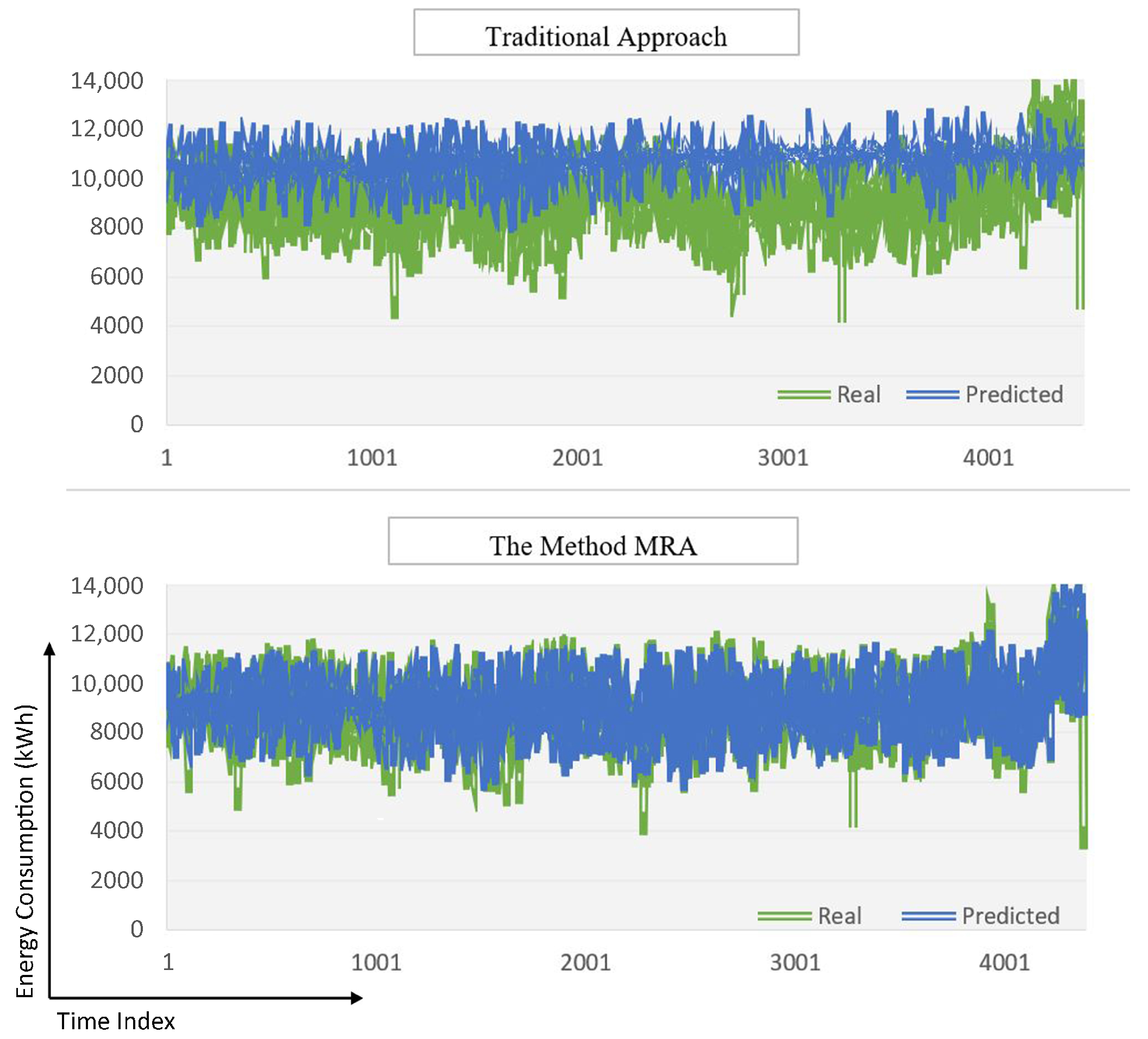
4.2. Experimental Results
5. Conclusions and Future Work
Author Contributions
Funding
Institutional Review Board Statement
Informed Consent Statement
Data Availability Statement
Conflicts of Interest
Nomenclature
| ANN | Artificial neural network |
| Bias | |
| C | Chunk no |
| CO2 | Carbon dioxide |
| dB | Decibel |
| DNN | Deep neural network |
| Err | Error rate |
| E | Error rate of the neural network |
| f | activation function |
| h | The number of hidden nodes |
| kWh | Kilowatt-hour |
| M | Model no |
| MAE | Mean absolute error |
| MAPE | Mean absolute percentage error |
| MRA | Multi-Regime approach |
| n | The number of input nodes |
| NC | Total number of chunks |
| NM | Number of models |
| psi | Pounds per square inch |
| PSF | Pattern sequence-based forecasting |
| ReLU | Rectified linear unit |
| RF | Random forest |
| RMSE | Root mean square error |
| SAG | Semi-autonomous grinding mill |
| SME | Subject matter expert |
| SVR | Support vector regression |
| The sum of the output variable | |
| t | Time index |
| tanh | Hyperbolic tangent function |
| Th | Threshold value |
| TPH | Ton per hour |
| Mill energy consumption values | |
| ,,, | The weights for the neural network connections |
| Wt | Window timing |
| The output variable | |
| Input variables |
Appendix A

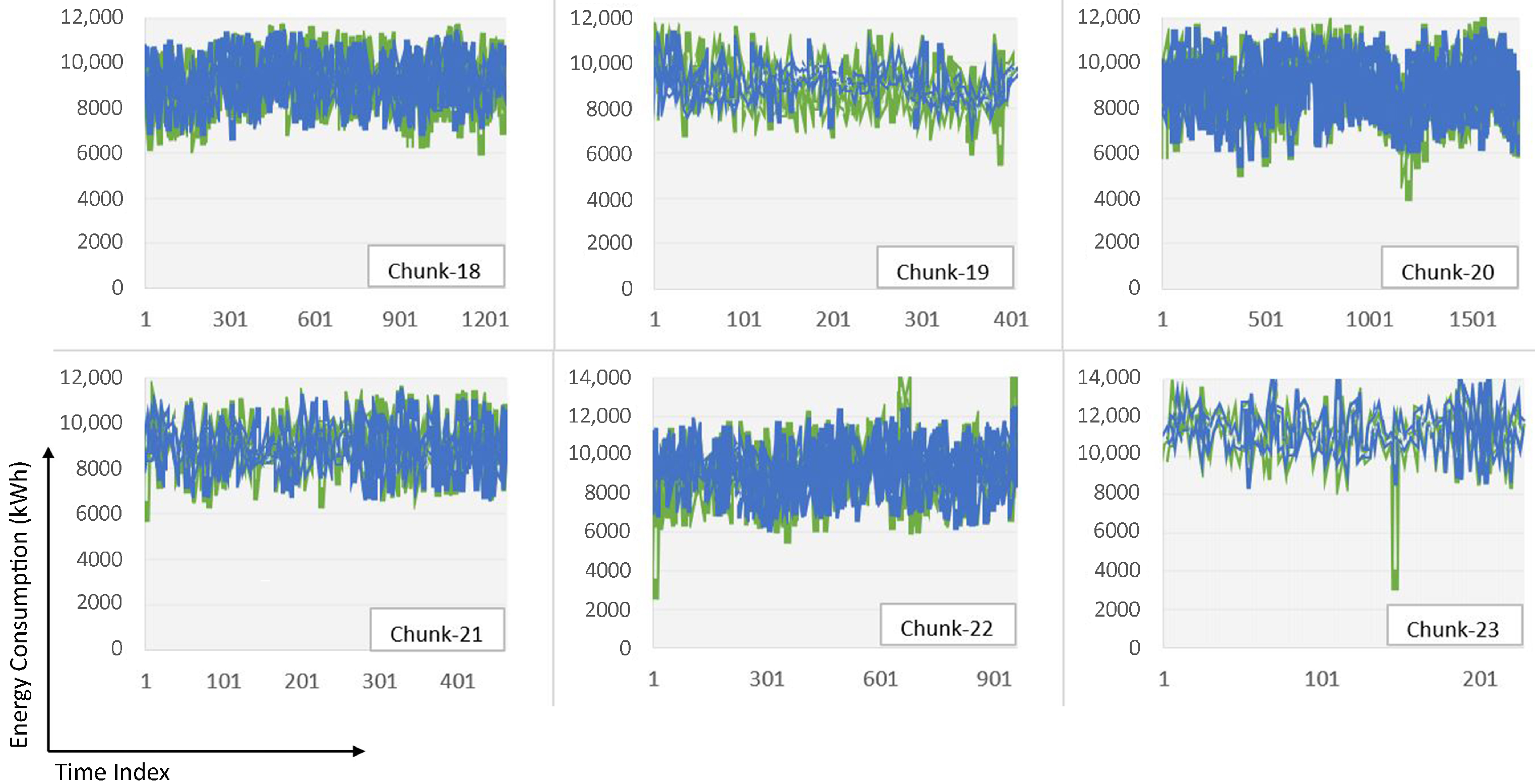
| Chunk No. | RMSE (kW) | MAE (kW) | MAPE | Model No. | Data Size | DNN Model Details |
|---|---|---|---|---|---|---|
| Chunk-1 | 558.606 | 399.851 | 4.07% | 1 | 884 | 4 layers each with 50 neurons, 80% training, 20% testing |
| Chunk-2 | 369.197 | 277.147 | 2.75% | 2 | 1134 | 3 layers each with 50 neurons, 80% training, 20% testing |
| Chunk-3 | 374.185 | 289.057 | 2.96% | 3 | 1006 | 3 layers each with 100 neurons, 80% training, 20% testing |
| Chunk-4 | 286.719 | 234.354 | 2.27% | 4 | 918 | 5 layers each with 50 neurons, 80% training, 20% testing |
| Chunk-5 | 251.755 | 191.603 | 1.85% | 5 | 449 | 4 layers each with 50 neurons, 70% training, 30% testing |
| Chunk-6 | 391.644 | 305.965 | 3.17% | 6 | 2338 | 5 layers each with 50 neurons, 80% training, 20% testing |
| Chunk-7 | 434.867 | 290.972 | 3.05% | 7 | 381 | 4 layers each with 100 neurons, 70% training, 30% testing |
| Chunk-8 | 374.29 | 270.084 | 2.86% | 8 | 535 | 4 layers each with 150 neurons, 70% training, 30% testing |
| Chunk-9 | 455.702 | 338.252 | 3.61% | 9 | 919 | 4 layers each with 50 neurons, 80% training, 20% testing |
| Chunk-10 | 293.248 | 235.917 | 2.48% | 10 | 624 | 4 layers each with 50 neurons, 70% training, 30% testing |
| Chunk-11 | 471.422 | 354.039 | 3.87% | 11 | 435 | 3 layers each with 50 neurons, 70% training, 30% testing |
| Chunk-12 | 336.583 | 261.434 | 2.74% | 12 | 306 | 3 layers each with 100 neurons, 70% training, 30% testing |
| Chunk-13 | 372.154 | 266.002 | 2.68% | 13 | 906 | 5 layers each with 50 neurons, 80% training, 20% testing |
| Chunk-14 | 527.264 | 389.147 | 3.90% | 14 | 689 | 4 layers each with 150 neurons, 70% training, 30% testing |
| Chunk-15 | 397.105 | 310.283 | 3.06% | 15 | 1138 | 4 layers each with 50 neurons, 80% training, 20% testing |
| Chunk-16 | 405.892 | 310.186 | 3.19% | 16 | 2871 | 4 layers each with 50 neurons, 70% training, 30% testing |
| Chunk-17 | 488.183 | 339.273 | 3.51% | 17 | 1711 | 3 layers each with 100 neurons, 70% training, 30% testing |
| Chunk-18 | 450.178 | 331.914 | 3.70% | 18 | 1272 | 4 layers each with 100 neurons, 70% training, 30% testing |
| Chunk-19 | 334.007 | 253.484 | 2.75% | 19 | 406 | 4 layers each with 50 neurons, 70% training, 30% testing |
| Chunk-20 | 465.403 | 345.34 | 3.99% | 20 | 1719 | 4 layers each with 100 neurons, 70% training, 30% testing |
| Chunk-21 | 283.137 | 227.15 | 2.53% | 21 | 462 | 5 layers each with 100 neurons, 70% training, 30% testing |
| Chunk-22 | 596.904 | 407.922 | 4.48% | 22 | 959 | 5 layers each with 100 neurons, 70% training, 30% testing |
| Chunk-23 | 272.855 | 209.01 | 1.83% | 23 | 228 | 3 layers each with 100 neurons, 70% training, 30% testing |
References
- Kim, J.Y.; Cho, S.B. Electric energy consumption prediction by deep learning with state explainable autoencoder. Energies 2019, 12, 739. [Google Scholar] [CrossRef] [Green Version]
- Zhao, G.; Liu, Z.; He, Y.; Cao, H.; Guo, Y. Energy consumption in machining: Classification, prediction, and reduction strategy. Energy 2017, 133, 142–157. [Google Scholar] [CrossRef]
- Kim, M.; Choi, W.; Jeon, Y.; Liu, L. A hybrid neural network model for power demand forecasting. Energies 2019, 12, 931. [Google Scholar] [CrossRef] [Green Version]
- Tan, M.; Yuan, S.; Li, S.; Su, Y.; Li, H.; He, F. Ultra-short-term industrial power demand forecasting using LSTM based hybrid ensemble learning. IEEE Trans. Power Syst. 2019, 35, 2937–2948. [Google Scholar] [CrossRef]
- Li, K.; Xue, W.; Tan, G.; Denzer, A.S. A state of the art review on the prediction of building energy consumption using data-driven technique and evolutionary algorithms. Build. Serv. Eng. Res. Technol. 2020, 41, 108–127. [Google Scholar] [CrossRef]
- Wang, X.; Yi, J.; Zhou, Z.; Yang, C. Optimal Speed Control for a Semi-Autogenous Mill Based on Discrete Element Method. Processes 2020, 8, 233. [Google Scholar] [CrossRef] [Green Version]
- Avalos, S.; Kracht, W.; Ortiz, J.M. Machine learning and deep learning methods in mining operations: A data-driven SAG mill energy consumption prediction application. Min. Metall. Explor. 2020, 37, 1197–1212. [Google Scholar]
- Silva, M.; Casali, A. Modelling SAG milling power and specific energy consumption including the feed percentage of intermediate size particles. Miner. Eng. 2015, 70, 156–161. [Google Scholar] [CrossRef]
- Curilem, M.; Acuña, G.; Cubillos, F.; Vyhmeister, E. Neural networks and support vector machine models applied to energy consumption optimization in semiautogeneous grinding. Chem. Eng. Trans. 2011, 25, 761–766. [Google Scholar]
- Yuwen, C.; Sun, B.; Liu, S. A Dynamic Model for a Class of Semi-Autogenous Mill Systems. IEEE Access 2020, 8, 98460–98470. [Google Scholar] [CrossRef]
- Hoseinian, F.S.; Abdollahzadeh, A.; Rezai, B. Semi-autogenous mill power prediction by a hybrid neural genetic algorithm. J. Cent. South Univ. 2018, 25, 151–158. [Google Scholar] [CrossRef]
- Hoseinian, F.S.; Faradonbeh, R.S.; Abdollahzadeh, A.; Rezai, B.; Soltani-Mohammadi, S. Semi-autogenous mill power model development using gene expression programming. Powder Technol. 2017, 308, 61–69. [Google Scholar] [CrossRef]
- Jnr, W.V.; Morrell, S. The development of a dynamic model for autogenous and semi-autogenous grinding. Miner. Eng. 1995, 8, 1285–1297. [Google Scholar]
- Hill, T.; O’Connor, M.; Remus, W. Neural network models for time series forecasts. Manag. Sci. 1996, 42, 1082–1092. [Google Scholar] [CrossRef]
- Park, J.; Law, K.H.; Bhinge, R.; Biswas, N.; Srinivasan, A.; Dornfeld, D.A.; Helu, M.; Rachuri, S. A generalized data-driven energy prediction model with uncertainty for a milling machine tool using Gaussian Process. In Proceedings of the International Manufacturing Science and Engineering Conference, Charlotte, NC, USA, 8–12 June 2015; American Society of Mechanical Engineers: Charlotte, NC, USA, 2015; Volume 56833, p. V002T05A010. [Google Scholar]
- Ceci, M.; Corizzo, R.; Japkowicz, N.; Mignone, P.; Pio, G. Echad: Embedding-based change detection from multivariate time series in smart grids. IEEE Access 2020, 8, 156053–156066. [Google Scholar] [CrossRef]
- Xu, W.; Peng, H.; Zeng, X.; Zhou, F.; Tian, X.; Peng, X. A hybrid modelling method for time series forecasting based on a linear regression model and deep learning. Appl. Intell. 2019, 49, 3002–3015. [Google Scholar] [CrossRef]
- Singh, S.; Yassine, A. Big data mining of energy time series for behavioral analytics and energy consumption forecasting. Energies 2018, 11, 452. [Google Scholar] [CrossRef] [Green Version]
- Demirel, Ö.F.; Zaim, S.; Çalişkan, A.; Özuyar, P. Forecasting natural gas consumption in Istanbul using neural networks and multivariate time series methods. Turk. J. Electr. Eng. Comput. Sci. 2012, 20, 695–711. [Google Scholar]
- Torres, J.F.; Hadjout, D.; Sebaa, A.; Martínez-Álvarez, F.; Troncoso, A. Deep Learning for Time Series Forecasting: A Survey. Big Data 2021, 9, 3–21. [Google Scholar] [CrossRef]
- Sezer, O.B.; Gudelek, M.U.; Ozbayoglu, A.M. Financial time series forecasting with deep learning: A systematic literature review: 2005–2019. Appl. Soft Comput. 2020, 90, 106181. [Google Scholar] [CrossRef] [Green Version]
- Mishra, S.; Bordin, C.; Taharaguchi, K.; Palu, I. Comparison of deep learning models for multivariate prediction of time series wind power generation and temperature. Energy Rep. 2020, 6, 273–286. [Google Scholar] [CrossRef]
- Manero, J.; Béjar, J.; Cortés, U. “Dust in the wind...”, deep learning application to wind energy time series forecasting. Energies 2019, 12, 2385. [Google Scholar] [CrossRef] [Green Version]
- Xiao, J.; Li, Y.; Xie, L.; Liu, D.; Huang, J. A hybrid model based on selective ensemble for energy consumption forecasting in China. Energy 2018, 159, 534–546. [Google Scholar] [CrossRef]
- Liu, X.; Chen, R. Threshold factor models for high-dimensional time series. J. Econom. 2020, 216, 53–70. [Google Scholar] [CrossRef] [Green Version]
- Battaglia, F.; Protopapas, M.K. Multi–regime models for nonlinear nonstationary time series. Comput. Stat. 2012, 27, 319–341. [Google Scholar] [CrossRef] [Green Version]
- Hu, H.; Kantardzic, M.; Sethi, T.S. No Free Lunch Theorem for concept drift detection in streaming data classification: A review. Wiley Interdiscip. Rev. Data Min. Knowl. Discov. 2020, 10, e1327. [Google Scholar] [CrossRef]
- McCandless, T.; Dettling, S.; Haupt, S.E. Comparison of implicit vs. explicit regime identification in machine learning methods for solar irradiance prediction. Energies 2020, 13, 689. [Google Scholar] [CrossRef] [Green Version]
- Lu, Z.; Xia, J.; Wang, M.; Nie, Q.; Ou, J. Short-term traffic flow forecasting via multi-regime modeling and ensemble learning. Appl. Sci. 2020, 10, 356. [Google Scholar] [CrossRef] [Green Version]
- Divina, F.; Garcia Torres, M.; Goméz Vela, F.A.; Vazquez Noguera, J.L. A comparative study of time series forecasting methods for short term electric energy consumption prediction in smart buildings. Energies 2019, 12, 1934. [Google Scholar] [CrossRef] [Green Version]
- Neto, A.H.; Fiorelli, F.A.S. Comparison between detailed model simulation and artificial neural network for forecasting building energy consumption. Energy Build. 2008, 40, 2169–2176. [Google Scholar] [CrossRef]
- Hamzaçebi, C. Improving artificial neural networks’ performance in seasonal time series forecasting. Inf. Sci. 2008, 178, 4550–4559. [Google Scholar] [CrossRef]
- Alvarez, F.M.; Troncoso, A.; Riquelme, J.C.; Ruiz, J.S.A. Energy time series forecasting based on pattern sequence similarity. IEEE Trans. Knowl. Data Eng. 2010, 23, 1230–1243. [Google Scholar] [CrossRef]
- Tso, G.K.; Yau, K.K. Predicting electricity energy consumption: A comparison of regression analysis, decision tree and neural networks. Energy 2007, 32, 1761–1768. [Google Scholar] [CrossRef]
- Hu, Y.C. Electricity consumption prediction using a neural-network-based grey forecasting approach. J. Oper. Res. Soc. 2017, 68, 1259–1264. [Google Scholar] [CrossRef]
- Kant, G.; Sangwan, K.S. Predictive modelling for energy consumption in machining using artificial neural network. Procedia CIRP 2015, 37, 205–210. [Google Scholar] [CrossRef]
- U.S. Energy Information Administration (EIA). Available online: www.eia.gov (accessed on 9 June 2021).
- Kankal, M.; Akpınar, A.; Kömürcü, M.İ.; Özşahin, T.Ş. Modeling and forecasting of Turkey’s energy consumption using socio-economic and demographic variables. Appl. Energy 2011, 88, 1927–1939. [Google Scholar] [CrossRef]
- Azadeh, A.; Ghaderi, S.F.; Tarverdian, S.; Saberi, M. Integration of artificial neural networks and genetic algorithm to predict electrical energy consumption. Appl. Math. Comput. 2007, 186, 1731–1741. [Google Scholar] [CrossRef]
- Wang, J.Q.; Du, Y.; Wang, J. LSTM based long-term energy consumption prediction with periodicity. Energy 2020, 197, 117197. [Google Scholar] [CrossRef]
- He, Y.; Wu, P.; Li, Y.; Wang, Y.; Tao, F.; Wang, Y. A generic energy prediction model of machine tools using deep learning algorithms. Appl. Energy 2020, 275, 115402. [Google Scholar] [CrossRef]
- Chen, C.; Liu, Y.; Kumar, M.; Qin, J. Energy consumption modelling using deep learning technique—A case study of EAF. Procedia CIRP 2018, 72, 1063–1068. [Google Scholar] [CrossRef]
- Lin, L.; Wang, F.; Xie, X.; Zhong, S. Random forests-based extreme learning machine ensemble for multi-regime time series prediction. Expert Syst. Appl. 2017, 83, 164–176. [Google Scholar] [CrossRef]
- Khashei, M.; Bijari, M. An artificial neural network (p, d, q) model for timeseries forecasting. Expert Syst. Appl. 2010, 37, 479–489. [Google Scholar] [CrossRef]
- Wei, N.; Li, C.; Peng, X.; Zeng, F.; Lu, X. Conventional models and artificial intelligence-based models for energy consumption forecasting: A review. J. Pet. Sci. Eng. 2019, 181, 106187. [Google Scholar] [CrossRef]


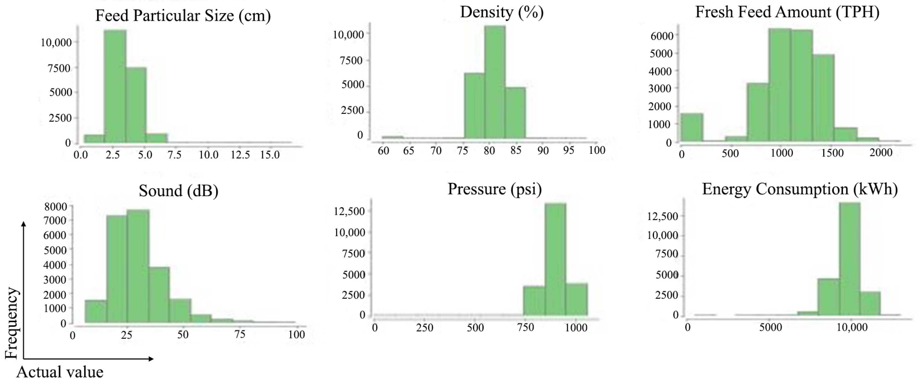
| Feed Particular Size (cm) | Mill Density (%) | Fresh Feed Amount (TPH) | Mill Sound (dB) | Mill Pressure (psi) | Mill Energy Consumption (kWh) | |
|---|---|---|---|---|---|---|
| Mean | 3.47 | 80.65 | 1069.23 | 30.26 | 895.61 | 9756.94 |
| Standard Deviation | 1.09 | 3.10 | 372.78 | 11.6 | 66.09 | 780.95 |
| Minimum | 0.28 | 60.02 | 0 | 7.04 | 240.895 | 492.60 |
| Maximum | 16.54 | 98.11 | 2196.72 | 99.1 | 1054.39 | 13,009.76 |
| Chunk No. | RMSE (kW) | MAE (kW) | MAPE | General MAPE Moving Average | Data Size |
|---|---|---|---|---|---|
| Chunk-1 | 558.606 | 399.851 | 4.07% | 4.07% | 884 |
| Chunk-2 | 482.829 | 377.286 | 3.76% | 3.92% | 1134 |
| Chunk-3 | 619.539 | 508.141 | 5.27% | 4.37% | 1006 |
| Chunk-4 | 636.746 | 478.183 | 6.72% | 4.96% | 918 |
| Chunk-5 | 471.063 | 385.239 | 3.77% | 4.72% | 449 |
| Chunk-6 | 599.276 | 477.449 | 5.03% | 4.77% | 2338 |
| Chunk-7 | 501.044 | 383.753 | 3.91% | 4.65% | 381 |
| Chunk-8 | 927.837 | 723.436 | 8.02% | 5.07% | 535 |
| Chunk-9 | 855.624 | 701.537 | 7.74% | 5.37% | 919 |
| Chunk-10 | 857.830 | 672.027 | 7.28% | 5.56% | 624 |
| Chunk-11 | 891.772 | 704.841 | 8.07% | 5.79% | 435 |
| Chunk-12 | 531.324 | 421.940 | 4.46% | 5.68% | 306 |
| Chunk-13 | 510.956 | 387.609 | 3.99% | 5.55% | 906 |
| Chunk-14 | 700.204 | 544.330 | 5.22% | 5.52% | 689 |
| Chunk-15 | 496.442 | 385.021 | 3.84% | 5.41% | 1138 |
| Chunk-16 | 957.800 | 811.572 | 8.63% | 5.61% | 2871 |
| Chunk-17 | 685.724 | 501.897 | 5.27% | 5.59% | 1711 |
| Chunk-18 | 1644.924 | 1464.499 | 16.67% | 6.21% | 1272 |
| Chunk-19 | 1647.166 | 1537.029 | 17.76% | 6.81% | 406 |
| Chunk-20 | 1771.213 | 1556.966 | 18.42% | 7.40% | 1719 |
| Chunk-21 | 1718.737 | 1616.370 | 18.36% | 7.92% | 462 |
| Chunk-22 | 1767.231 | 1628.439 | 18.43% | 8.40% | 959 |
| Chunk-23 | 1053.187 | 811.229 | 7.33% | 8.35% | 228 |
| Chunk No. | RMSE (kW) | MAE (kW) | MAPE < Threshold (10%) | General MAPE Moving Average | Data Size | Regime-Model No. | Are There Any Old Models? |
|---|---|---|---|---|---|---|---|
| Chunk-1 | 558.606 | 399.851 | 4.07% | 4.07% | 884 | 1 | No |
| Chunk-2 | 482.829 | 377.286 | 3.76% | 3.92% | 1134 | 1 | No |
| Chunk-3 | 619.539 | 508.141 | 5.27% | 4.37% | 1006 | 1 | No |
| Chunk-4 | 636.746 | 478.183 | 6.72% | 4.96% | 918 | 1 | No |
| Chunk-5 | 471.063 | 385.239 | 3.77% | 4.72% | 449 | 1 | No |
| Chunk-6 | 599.276 | 477.449 | 5.03% | 4.77% | 2338 | 1 | No |
| Chunk-7 | 501.044 | 383.753 | 3.91% | 4.65% | 381 | 1 | No |
| Chunk-8 | 927.837 | 723.436 | 8.02% | 5.07% | 535 | 1 | No |
| Chunk-9 | 855.624 | 701.537 | 7.74% | 5.37% | 919 | 1 | No |
| Chunk-10 | 857.830 | 672.027 | 7.28% | 5.56% | 624 | 1 | No |
| Chunk-11 | 891.772 | 704.841 | 8.07% | 5.79% | 435 | 1 | No |
| Chunk-12 | 531.324 | 421.940 | 4.46% | 5.68% | 306 | 1 | No |
| Chunk-13 | 510.956 | 387.609 | 3.99% | 5.55% | 906 | 1 | No |
| Chunk-14 | 700.204 | 544.330 | 5.22% | 5.52% | 689 | 1 | No |
| Chunk-15 | 496.442 | 385.021 | 3.84% | 5.41% | 1138 | 1 | No |
| Chunk-16 | 957.800 | 811.572 | 8.63% | 5.61% | 2871 | 1 | No |
| Chunk-17 | 685.724 | 501.897 | 5.27% | 5.59% | 1711 | 1 | No |
| Chunk-18 | 1644.924 | 1464.499 | 16.67% | 6.21% | 1272 | 1 | No |
| Chunk-18 | 450.178 | 331.914 | 3.70% | 5.49% | 1272 | 2 | Yes |
| Chunk-19 | 387.165 | 287.935 | 3.17% | 5.36% | 406 | 2 | Yes |
| Chunk-20 | 1172.610 | 981.431 | 10.67% | 5.63% | 1719 | 2 | Yes |
| Chunk-20 | 1771.213 | 1556.966 | 18.42% | 6.02% | 1719 | 1 | No |
| Chunk-20 | 465.403 | 345.34 | 3.99% | 5.30% | 1719 | 3 | Yes |
| Chunk-21 | 623.416 | 525.236 | 5.74% | 5.32% | 462 | 3 | Yes |
| Chunk-22 | 1125.931 | 784.768 | 8.20% | 5.45% | 959 | 3 | Yes |
| Chunk-23 | 2354.083 | 2272.379 | 20.14% | 6.09% | 228 | 3 | Yes |
| Chunk-23 | 1053.187 | 811.229 | 7.33% | 5.53% | 228 | 1 | Yes |
Publisher’s Note: MDPI stays neutral with regard to jurisdictional claims in published maps and institutional affiliations. |
© 2021 by the authors. Licensee MDPI, Basel, Switzerland. This article is an open access article distributed under the terms and conditions of the Creative Commons Attribution (CC BY) license (https://creativecommons.org/licenses/by/4.0/).
Share and Cite
Kahraman, A.; Kantardzic, M.; Kahraman, M.M.; Kotan, M. A Data-Driven Multi-Regime Approach for Predicting Energy Consumption. Energies 2021, 14, 6763. https://doi.org/10.3390/en14206763
Kahraman A, Kantardzic M, Kahraman MM, Kotan M. A Data-Driven Multi-Regime Approach for Predicting Energy Consumption. Energies. 2021; 14(20):6763. https://doi.org/10.3390/en14206763
Chicago/Turabian StyleKahraman, Abdulgani, Mehmed Kantardzic, Muhammet Mustafa Kahraman, and Muhammed Kotan. 2021. "A Data-Driven Multi-Regime Approach for Predicting Energy Consumption" Energies 14, no. 20: 6763. https://doi.org/10.3390/en14206763
APA StyleKahraman, A., Kantardzic, M., Kahraman, M. M., & Kotan, M. (2021). A Data-Driven Multi-Regime Approach for Predicting Energy Consumption. Energies, 14(20), 6763. https://doi.org/10.3390/en14206763